Dragging a polymer chain into a nanotube and subsequent release

Abstract

We present a scaling theory and Monte Carlo (MC) simulation results for a flexible polymer chain slowly dragged by one end into a nanotube. We also describe the situation when the completely confined chain is released and gradually leaves the tube. MC simulations were performed for a self-avoiding lattice model with a biased chain growth algorithm, the pruned-enriched Rosenbluth method (PERM). The nanotube is a long channel opened at one end and its diameter $D$ is much smaller than the size of the polymer coil in solution. We analyze the following characteristics as functions of the chain end position $x$ inside the tube: the free energy of confinement, the average end-to-end distance, the average number of segments imprisoned in the tube, and the average stretching of the confined part of the chain for various values of $D$ and for the number of repeat units in the chain, $N$. We show that when the chain end is dragged by a certain critical distance $x^{*}$ into the tube, the polymer undergoes a first-order phase transition whereby the remaining free tail is abruptly sucked into the tube. This is accompanied by jumps in the average size, the number of imprisoned segments, and in the average stretching parameter. The critical distance scales as $x^{*}\sim ND^{1-1/\nu}$. The transition takes place when approximately $3/4$ of the chain units are dragged into the tube. The theory presented is based on constructing the Landau free energy as a function of an order parameter that provides a complete description of equilibrium and metastable states. We argue that if the trapped chain is released with all monomers allowed to fluctuate, the reverse process in which the chain leaves the confinement occurs smoothly without any jumps. Finally, we apply the theory to estimate the lifetime of confined DNA in metastable states in nanotubes.

I Introduction

Recent developments in fabrication of nanoscale devices and in single-chain manipulation techniques open possibilities for a broad range of applications in biotechnology and materials science Salman ; Meller ; Kasianowicz ; Aktson ; Meller00 ; Clausen ; Williams . In particular, well calibrated nanochannels were produced in fused silica substrates by lithography methods with the widths in the range of $30$ to $400$ nm, which were used to study the confinement of single $\lambda$-phage DNA molecules driven electrophoretically into these nanochannels Reisner . The persistence length of DNA under conditions used in these experiments is about $50$ nm while its contour length was about $1000$ times larger. This means that except for the case of the narrowest channels DNA behaved essentially as a long flexible macromolecule on the relevant length scales. The aim of this paper is to elucidate the subtle physics behind the process when a long flexible chain is slowly dragged by one end into a nanochannel. We also show that this process is qualitatively different from what happens when a confined chain is released and leaves the nanochannel by spontaneous thermal motion.

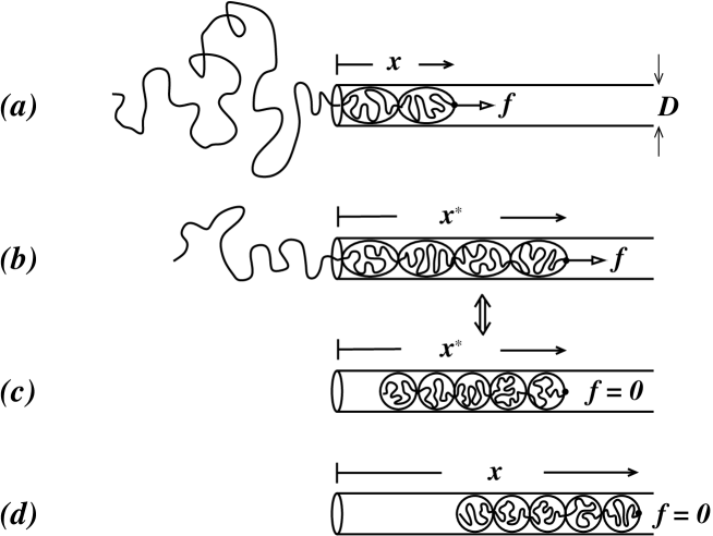
Figure 1: Schematic drawings of a flexible polymer chain with one end dragged into a nanotube in a quasi-equilibrium process. The fixed chain end characterized by its coordinate $x$ experiences an reaction force $f$ that balances the pull of the undeformed swollen coil outside the tube (a)(b). At the transition point $x^{*}$, the remaining tail is sucked into the tube abruptly by a uniform shrinking of all blobs in the stem (b), (c), and the reaction force becomes zero, $f=0$. At the transition point conformations (b) and (c) coexist. As long as the chain is fully confined in the tube, no reaction force appears at the fixed chain end (d).

Our approach is based on using the most general results of the scaling theory that neglect the small-scale details of the system under consideration, namely the particular form of the interaction potentials, the flexibility mechanisms, etc. It is well known that the scaling approach does not allow to calculate non-universal numerical coefficients that are model-dependent. To verify the prediction of the analytical theory we have carried out detailed Monte Carlo (MC) simulation by using the pruned-enriched Rosenbluth method (PERM) g97 ; Hsu03 ; Hsu04 ; Hsu07 . The simulations are based on the simplest model of polymers, namely self-avoiding walks on a cubic lattice. Fortunately, the general ideas of scaling guarantee a universal behavior within broad limits of parameters.

The properties of a single macromolecule confined in a tube have been studied extensively for decades, both by analytical theory and by numerical simulations for various models of flexible and semi-flexible chains Kremer ; Sotta ; Milchev94 ; Yang . For a homogeneous confined state there are scaling predictions Daoud concerning various chain characteristics which were tested by MC simulations. Our main interest here is in the non-homogeneous flower-like states where the confined part of the chain inside the tube forms a stretched stem and the free tail still in solution forms a coiled crown. This type of conformations appears in a variety of situations including translocation through a thick membrane Randel as well as the escape transition produced by compressing a grafted chain between flat pistons Subra ; Ennis99 ; Sevick99 ; Steels ; Milchev . One of the goals of this paper is to demonstrate that the role of these conformations in the situations mentioned above are quite different depending on whether one of the chain ends is fixed in the confinement region or not.

The paper is organized as follows: We start by presenting the main qualitative results in a series of simple pictures visualizing the conformational changes in the process of dragging the chain end slowly into the tube and its de-confinement upon subsequent release. In Section III we give the results of the MC simulations for completely confined states and compare them with the well-known scaling prediction. Section IV describes the simulation results characterizing the phase transition induced by changing the chain end position inside the tube. In Section V we provide a theoretical description of the phenomenon based on the Landau free energy approach and compare it to the MC results. The process of spontaneous de-confinement is analyzed in Section VI and followed by a general discussion.

Figure 2: Schematic drawings of a released flexible polymer chain. Since all the chain units are free to fluctuate, no reaction force is needed to counterbalance the force due to the tail outside the tube. The stretching of the stem is only dependent on the confinement effect at any moment, (a) and (b).

II Qualitative picture

Figure 1 presents a sequence of chain conformations when the position of one of the chain ends is progressively moved quasi-statically further inside the nanotube. At each moment, this fixed chain end is characterized by its coordinate $x$ which is controlled externally. The tail outside the tube is a practically undeformed swollen coil while the part of the chain inside forms a one-dimensional string of blobs. The chain can be presented as a flower structure with one-dimensional structure of the stem. The number of confined (imprisoned) chain units grows linearly with $x$, at least in the initial stages of the process. The fixed chain end experiences a force which is due to the tail still not being confined. To counterbalance this force, a reaction force $f$ directed into the tube will appear. Once the chain is confined completely (Figures 1c and 1d) there is no tail outside the tube and the reaction force at the controlled chain end disappears. In this state, the chain is homogeneously stretched and its stretching degree is due solely to the confinement effect Daoud . It is clear that the stem of the partially confined conformation is stretched more strongly since the confinement effects are augmented by the additional stretching force (this effect is symbolically indicated by the deformation in blob shape shown in the Figures 1a and 1b). The difference in the deformation free energy leads to a phase transition - an abrupt “slurping” of the remaining tail accompanied by a uniform shrinking of all blobs in the stem. (Of course, in a strict sense true phase transitions can occur only in the thermodynamic limit, which would require that both the length of the chain and the length of the pore are infinitely large; however, as we shall see, the rounding of the phase transition caused by finite chain length is not too significant.) As a result the length along the tube of the completely confined chain is less than the length of the stem just before the transition, as illustrated in Figures 1b and 1c. Note that the process described above has to be distinguished from the case when the chain is driven into the pore by applying a constant force, as in electrophoresis.

The next figure (Figure 2) illustrates the de-confinement of a released chain. All the chain units are free to fluctuate and there is no reaction force. Therefore, the stem stretching is only due to the confinement effect at any particular moment. The gradual decrease in the number of imprisoned units is not accompanied by any jumps.

III Fully confined chain: MC results and scaling

The scaling picture of a fully confined chain inside a tube of diameter $D$ is very simple. It is formed by a string of non-overlapping blobs of size $\sim D$, each blob containing $g$ monomer units Daoud . The size of the blob is related to $g$ by

$$D\sim ag^{\nu}$$ (1)

where $a$ is the length of a monomer unit, and $\nu=0.58765(20)$ is the scaling index for a three-dimensional self-avoiding chain Hsu04 . Let’s define the number of blobs by relation

$$n_{b}=N/g=N(D/a)^{-1/\nu}\;.$$ (2)

In this case the average end-to-end distance of the chain in a fully confined (imprisoned) state is

$$R_{\rm imp}=A_{\rm imp}Dn_{b}$$ (3)

where $A_{\rm imp}$ is a model-dependent numerical coefficient. In eqs 1-3 we have assumed that the pore diameter $D$ is large enough, so that the number of monomers inside a single blob is large enough so that the scaling relation eq 1 holds; further more correction terms to the scaling relations are omitted throughout.

Figure 3: (a) Rescaled average end-to-end distance $R_{\rm imp}/(n_{b}D)$ against the number of blobs $n_{b}=N(D/a)^{-1/\nu}$ for fully confined chains. The thick solid line with arrow is $R_{\rm imp}/(n_{b}D)=A_{\rm imp}$ with $A_{\rm imp}=0.92(3)$. (b) The log-log plot of the same data as (a) shows that for $n_{b}>2$ the data collapse and allows to estimate $A_{\rm imp}$ very accurately. The dotted straight line with slope $\nu-1$ shows the scaling law in the regime of wide tubes with $D>R_{\rm imp}$.

Figure 4: (a) Rescaled average free energy $F_{\rm imp}/n_{b}$ for fully confined chains against the number of blobs $n_{b}$ . The thick solid line with arrow is $F_{\rm imp}/n_{b}=B_{\rm imp}$ with $B_{\rm imp}=5.33(5)$. (b) Same as (a), but on a log-log plot to show that for $n_{b}>1$ the data allows to estimate $B_{\rm imp}$ very accurately.

A stretching parameter $S_{\rm imp}=R_{\rm imp}/Na$ describes the average stretching of the chain in an imprisoned state. Since the end-to-end distance of the fully imprisoned chain is proportional to $N$, the stretching parameter is a function of the tube diameter only and is given by

$$S_{\rm imp}=A_{\rm imp}(D/a)^{1-1/\nu}\;.$$ (4)

For a fully imprisoned chain the free energy of confinement per blob scales as $k_{B}T$. Thus, using eq 2 the free energy of a fully imprisoned chain is

$$F_{\rm imp}=B_{\rm imp}n_{b}$$ (5)

where $B_{\rm imp}$ is another numerical coefficient. The factor of $k_{B}T$ is absorbed in the free energy throughout the paper hereafter.

For our simulations, chain lengths are up to 44000, tube diameters are up to $D=97$, and $a=1$ which is the lattice spacing. Simulation data for the rescaled average root mean square (rms) end-to-end distance $R_{\rm imp}/(n_{b}D)$ are displayed in Figure 3 depending on the blob number $n_{b}$. It is evident from the Figure 3 that the normalized chain size reaches a practically constant value when the chain contains more than two blobs. The limiting constant value of $R_{\rm imp}/(n_{b}D)$ is just the numerical coefficient $A_{\rm imp}=0.92\pm 0.03$ in eq 3. As noted above, the scaling description is expected to become exact in the asymptotic limit $D\rightarrow\infty$, and hence in the considered range of not very large $D$ a small systematic dependence of the curves in Figure 3a is evident, leading to the spread of values of the coefficient $A_{\rm imp}$, as expressed by the quoted uncertainty. Figure 3 shows that at values $n_{b}<1$, the unperturbed coil size smaller than the tube diameter, there is another scaling regime of weak confinement where $R_{\rm imp}\sim N^{\nu}$. Although the crossover between these two regimes is of general theoretical interest, we are not concerned with it in this paper.

The rescaled free energy $F_{\rm imp}$ (counted from the reference state of a self-avoiding coil in free space) for the fully imprisoned chain is presented in Figure 4 vs. the number of blobs $n_{b}$. The limiting constant value gives the coefficient $B_{\rm imp}=5.33\pm 0.08$ in eq 5, which represents the free energy per blob in $k_{B}T$ units. Once again we see the other scaling regime of weak confinement if the number of blobs in the chain is less then one blob. Summarizing the presented data we can conclude that using the definition of the number of blobs given by eq 2 the size of the blob in our model is close to $D$, the end-to-end distance $R_{\rm imp}\sim 0.92n_{b}D$, and the free energy per blob $F_{\rm imp}/n_{b}\sim 5.33$ is close to 5 $k_{B}T$. Comparing our result for the free energy per blob, $F_{\rm tube}/n_{b}$ $(F_{\rm tube}=F_{\rm imp})$ with that of chains confined in a slit on a lattice Hsu04 , $F_{\rm slit}/n_{b}\sim 2.10$, and a off-lattice model Dimitar , $F_{\rm slit}/n_{b}\sim 2.03$, we find that $F_{\rm tube}\approx 2F_{\rm slit}$. It is not surprising because a polymer chain confined in a slit is compressed in one direction and in a tube in two directions.

Figure 5: Free energy of chains with chain lengths $N=500$ and $N=1500$ relative to a self-avoiding coil, $F(N,x,D)$, plotted against $x/D$ for tube diameters $D=17$, $21$ and $25$. The solid straight line is $F_{\rm fl}=4.23x/D$ and gives the best fit of the data of chains in a flower state. All horizontal lines indicate the values of $F_{\rm imp}$ for chains in an imprisoned state at fixed chain length $N$. The intersections of the solid line and horizontal lines indicate the transition points $x^{*}/D$.

Figure 6: Transition points $x^{*}$ as obtained from Figures 5, plotted against $N(D/a)^{1-1/\nu}$ for various values of $N$ and $D$. The dotted line has slope $B_{\rm imp}/B_{\rm fl}=1.25$ .

IV Phase transition: equilibrium characteristics

For our simulations, single polymer chains are dragged into a tube with diameters $D=17$, $21$, $25$, and $29$, and the chain length is up to $N=17000$. Simulation results of the free energy relative to a self-avoiding coil are presented in Figure 5 as a function of the end monomer position inside the tube, $x$, normalized by the tube diameter $D$. It is clear that there are two branches of the free energy. Initially, the free energy increases linearly with $x$ as more and more blobs are driven into the tube. The slope of the free energy as a function of $x$ has the meaning of the average reaction force acting on the end monomer. Deviations from the linearity near the origin occur when only the number of blobs inside the tube is of order one or less. At large enough values of $x$ all monomeric units are confined and the free energy does not depend on the position $x$ any more. An abrupt change in the slope of the free energy indicates a first-order transition. The linear branch describes a partially confined “flower” state. On this branch the data points for different values of $N$ and $D$ collapse onto the same universal curve in the chosen coordinates. The $x$-independent branch corresponds to a completely confined state discussed above in Section III. Altogether the results can be summarized as follows:

$$F(N,x,D)=\left\{\begin{array}[]{ll}B_{\rm imp}N(D/a)^{-1/\nu}=F_{\rm imp}&\enspace{\rm imprisoned\,state}\\ B_{\rm fl}(x/D)=F_{\rm fl}&\enspace{\rm flower\,state}\end{array}\right.\;.$$ (6)

where $B_{\rm imp}=5.33(8)$ and $B_{\rm fl}=4.23(6)$ were obtained from Figure 4 and Figure 5. Physically, both formulas state that the free energy is proportional to the number of blobs inside the tube. However, we would like to point out that the numerical coefficients are different, and the most important source of this difference is due to the extra stretching of the flower stem as compared to the relaxed fully confined state.

Figure 7: (a) Average fraction of imprisoned units, $N_{\rm imp}/N$, plotted against the reduced end coordinate $x/x^{*}$ for $n_{b}=60$ and for various values of $D$. The solid line gives the theoretical prediction that the fraction increases linearly with $x$ below the transition point, and it is in perfect agreement with our data. At the transition point $x/x^{*}=1$, $N_{\rm imp}/N$ jumps up from $0.76$ to $1$, and the relative reduction in the number of imprisoned monomers is then $\Delta_{N}\approx 0.24$. (b) $N_{\rm imp}/N$ vs. $x/x^{*}$ the transition region, $x/x^{*}=1$, for $D=21$ and for different number of $n_{b}$, displaying the rounding of the transition is due to the finiteness of the number of blobs.

Figure 8: (a) Reduced rms end-to-end distance $R/R_{\rm imp}$, plotted against the reduced end coordinate $x/x^{*}$ for $n_{b}=60$ and for various values of $D$. $R_{\rm imp}$ is the average rms end-to-end distance for a fully confined chain. Near $x=0$, chains behave as a self-avoiding coil, $R/R_{\rm imp}$ depends on both $N$ and $D$. Approaching the transition point from below, a linear behavior appears according to the scaling prediction. At the transition point $x/x^{*}=1$, the value of $R/R_{\rm imp}$ jumps down from $1.38$ to $1$ and the reduced jump of end-to-end distance $\Delta_{R}=(1.38-1)/1.38\approx 0.27$. (b) $R/R_{\rm imp}$ vs. $x/x^{*}$ around the transition region, $x/x^{*}=1$, for $D=21$ and for different number of $n_{b}$.

Figure 9: (a) Reduced average stretching parameter $<s>/S_{\rm imp}$, plotted against the reduced end coordinate $x/x^{*}$ for $n_{b}=60$ and for various values of $D$. $S_{\rm imp}$ is the average stretching of a fully confined chain, and it does not depend on $x/x^{*}$. The average stretching of the chain in a flower state is the stretching of the stem and it is also independent of $x/x^{*}$ except the region that near $x=0$ where it depends on both $N$ and $D$. At the transition point $x/x^{*}=1$, the value $<s>/S_{\rm imp}$ jumps down from $1.75$ to $1$ and the reduced jump of the stretching parameter is $\Delta_{S}=(1.75-1)/1.75\approx 0.43$. (b) $<s>/S_{\rm imp}$ vs. $x/x^{*}$ around the transition region, $x/x^{*}=1$, for $D=21$ and for different number of blobs $n_{b}$.

The intersection of the two free energy branches defines the transition point, or the critical distance $x^{*}$ away from the open end of the tube. Equating the two expressions of eq 6 one obtains:

$$x^{*}=(B_{\rm imp}/B_{\rm fl})N(D/a)^{1-1/\nu}=1.26(4)N(D/a)^{1-1/\nu}$$ (7)

MC data for the transition points displayed in Figure 6 are in full agreement with eq 7.

The average fraction of imprisoned units, $N_{\rm imp}/N$, as a function of the reduced end coordinate $x/x^{*}$ is shown in Figure 7. It is clear that this fraction increases linearly with $x$ and jumps up to $1$ at the transition point. This jump represents the abrupt “slurping” of the tail which constitutes approximately $1/4$ of the total number of units, $N$. As mentioned above, truly sharp jumps can occur in the thermodynamic limit $(N\rightarrow\infty)$ only, so when one looks at the behavior of $N_{\rm imp}/N$ with high resolution on the scale $x/x^{*}$ for various sizes of the system, one can resolve the finite-size rounding (Figure 7b). The next graph (Figure 8) represents the change in the rms end-to-end distance reduced by the corresponding value for the completely confined chain, $R/R_{\rm imp}$. The starting value at $x=0$ represents an unconfined coil with $R\approx N^{\nu}$ so that the reduced value depends on both $N$ and $D$, i.e., $R/R_{\rm imp}\propto N^{\nu}/(ND^{1-1/\nu})$. Then, a linear dependence appears which is terminated at the transition point. The average size jumps down by approximately $25\%$. Finally, the average stretching parameter $<s>$ of the confined part of the chain is shown in Figure 9 as a function of the same reduced distance $x/x^{*}$. (For the precise definition of the stretching parameter $s$, see the next section). It is reduced by the value $S_{\rm imp}$ characterizing the fully confined chain, independent of $x$ and given by eq 4. In a flower state the stretching parameter $S_{\rm fl}$ describes the average stretching of the stem. It is independent of $x$ also and is about $1.75$ times larger than that for the fully confined chain. A small deviation exists near $x=0$ only. Beyond the transition point $S_{\rm fl}$ jumps down to the $S_{\rm imp}$ value.

V Landau theory

Unlike the case of critical phenomena, the Landau theory approach is very well suited for analyzing first-order transitions, including possible metastable states. The idea is to first subdivide all configurations into subsets associated with a given value of an appropriately chosen order parameter $s$ that allows to distinguish between different states or phases. Landau free energy $\Phi(s)$ is the free energy of a given subset, and is therefore a function of the order parameter. The minimum value of the Landau free energy is attained for the subset that contains most of the equilibrium configurations, and therefore coincides with the equilibrium free energy of the system, $F$. Far enough from the first order transition point, the Landau free energy has only one minimum. However, near the transition the function is expected to have two minima (the deeper one is stable and the other is metastable). Exactly at the transition point, both minima are of equal depth. We define the order parameter as the chain stretching in the fully confined state, $s=r/(N_{\rm imp}a)$ ($N_{\rm imp}=N$) where $r$ is the instantaneous end-to-end distance of the chain, or as the stretching of the stem only in the flower state, $s=x/(na)$ where $n$ is the instantaneous number of confined monomers in the stem, and $x$ is the length of the stem. The Landau function consists of two branches that have to be introduced separately. For fully confined configurations the Landau free energy, up to an additive constant, is directly expressed in terms of the distribution of the end-to-end distance $P(r|N,D)$ of a chain in the tube:

$$\Phi_{\rm imp}(r/Na)=const-\ln P(r|N,D)\;.$$ (8)

There exists no closed formula for such a distribution of confined chains with excluded volume interactions. In Ref. Sotta the (non-normalized) distribution for the gyration radius was studied numerically and the following scaling form was proposed:

$$\ln P(R_{g}|N,D)=-N(D/a)^{-1/\nu}A\left[u^{-\alpha}+Bu^{\delta}\right]$$ (9)

where $\alpha=(3\nu-1)^{-1}$ , $\delta=(1-\nu)^{-1}$ and $u={(R_{g}/Na)}(D/a)^{{-1+1/\nu}}$. The parameters $A$ and $B$ are non-universal numbers of order unity and they do not depend on $N$ or $D$. The first term describes the concentration effects in the des Cloizeaux Cloizeaux form, and the second term is the Pincus Pincus scaling form of the stretching free energy. From our MC simulations, we have found that the end-to-end distribution $P(r|N,D)$ and the equilibrium free energy $F$ are well described by a similar scaling formula corrected by an additional $r$-independent term, namely the Landau free energy for the imprisoned state is then

$$\Phi_{\rm imp}(s)=N(D/a)^{-1/\nu}A\left[u^{-\alpha}+Bu^{\delta}+C\right]$$ (10)

where $u$ is now related to our order parameter $s$

$$u={(r/Na)}(D/a)^{{-1+1/\nu}}=s(D/a)^{-1+{1/\nu}}\;.$$ (11)

This branch is limited to the range of values for the order parameter,   $0<s<x/Na$.    In the thermodynamic limit, the average value of the order parameter of a fully confined chain, $S_{\rm imp}=<s>$, is found by locating the minimum of $\Phi_{\rm imp}(s)$, i.e., $d\Phi_{\rm imp}(s)/ds=0$ at $s=S_{\rm imp}$, and the corresponding minimum of the Landau free energy is the equilibrium free energy $F$. Using eq 11, we obtain the equilibrium average value of the end-to-end distance $R_{\rm imp}=<r>$,

$$R_{\rm imp}=N<s>=N(D/a)^{1-{1/\nu}}u_{1}$$ (12)

where $u_{1}=(\alpha/\delta B)^{1/(\alpha+\delta)}$ gives the position of the minimum of the function $f(u)=u^{-\alpha}+Bu^{\delta}+C$. Comparing this result with the MC data of $D=17$, i.e. eq 3 with taking $A_{\rm imp}=0.94$, we immediately determine the numerical value of $B=0.67$. Using eq 10, the equilibrium free energy $F_{\rm imp}$ is the Landau free energy at $u=u_{1}$:

$$F_{\rm imp}=N(D/a)^{-1/\nu}A\left(1.67+C\right)$$ (13)

Comparing this again with the MC data of $D=17$, i.e. eq 5 with taking $B_{\rm imp}=5.38$, we get a relationship between the coefficients $A$ and $C$. The last condition that eventually fixes all the numerical coefficients $A$, $B$ and $C$ of the Landau function is obtained by analyzing its second branch.

For the partially confined chains in the flower state, since in fact only $n$ monomers that comprise the stem of the flower give contributions to the free energy, instead of $N$ and $r$, we use $n$ and $x$ in eq 10. The formula of the Landau free energy is therefore,

$$\Phi_{\rm fl}(s) = \frac{x}{D}A\left[u^{-\alpha-1}+Bu^{\delta-1}+Cu^{-1}\right],\enspace s\geq\frac{x}{N}\;.$$ (14)

where $u$ is given by

$$u={(x/na)}(D/a)^{{-1+1/\nu}}=s(D/a)^{-1+{1/\nu}}\;.$$ (15)

The average value of the order parameter $S_{\rm fl}$, and the equilibrium free energy $F_{\rm fl}$ for the flower state are obtained by the same procedure as that for the imprisoned state. Demanding that $S_{\rm fl}$ and the coefficient with the $x/D$ factor in eq 14 both coincide with the MC results, we are uniquely fixing the numerical values of parameters $A=1.48$, $B=0.67$ and $C=1.98$.

Figure 10: Landau free energy divided by $N$, $\Phi(N,x,D,s)/N$, plotted against the order parameter $s$ for various values of $x/x^{*}$ and for $D=17$ (a) and $D=21$ (b). The predicted Landau free energy function $\Phi_{\rm imp}$, eq 10, in the imprisoned regime, and $\Phi_{\rm fl}$, eq 14, in the flower regime, with $A=1.48$, $B=0.67$, and $C=0.98$, give a good fit to the MC data.

VI Comparison with MC results.

For our simulations, the Landau free energy as a function of $s$, $\Phi(N,x,D,s)$, is given by taking the logarithm of the properly normalized accumulated histogram of stretching parameter $s$. Results for tubes with diameters $D=17$ and $D=21$ near the transition point $x^{*}/Na\sim 1.26(D/a)^{1-1/\nu}$ {eq 7} are shown in Figure 10. Two branches of the analytical Landau function given by eqs 10 and 14 for $A=1.48$, $B=0.67$, and $C=1.98$ are also presented in Figure 10. We see that in both the flower and the imprisoned states, MC data are in perfect agreement with the theoretical predictions for a wide range of $s$ at any $x$, and $D$ although the coefficients $A$, $B$, and $C$ are determined by using only the MC estimates of average stretching parameters $S_{\rm imp}$ and $S_{\rm fl}$ , and of average free energies $F_{\rm imp}$ and $F_{\rm fl}$ for $D=17$.

From the analytical Landau function in the imprisoned state and in the flower state, eqs 10 and 14, and the determined values of the coefficients $A$, $B$, and $C$, we obtain the following scaling relationships of the equilibrium order parameters $s$

$$s=s_{eq}=\left\{\begin{array}[]{ll}0.94(D/a)^{1-1/\nu}=S_{\rm imp}&\enspace{\rm imprisoned\,state}\\ 1.64(D/a)^{1-1/\nu}=S_{\rm fl}&\enspace{\rm flower\,state}\\ \end{array}\right.\;,$$ (16)

and the equilibrium free energies $F$,

$$F_{eq}=\left\{\begin{array}[]{ll}5.40N(D/a)^{-1/\nu}=F_{\rm imp}&\enspace{\rm imprisoned\,state}\\ 4.27x/D=F_{\rm fl}&\enspace{\rm flower\,state}\\ \end{array}\right.$$ (17)

The transition point is found from the condition that the two minima of the Landau free energy function are of equal depth. Using eqs 17 we get

$$\frac{x_{tr}}{Na}\sim 1.26(D/a)^{1-1/\nu}$$ (18)

The reduced jump of the order parameter is therefore

$$\Delta_{S}=\frac{S_{\rm fl}-S_{\rm imp}}{S_{\rm fl}}\approx 0.43\;.$$ (19)

The average number of units dragged into the tube for an imprisoned state is $N_{\rm imp}=N$, while for the coexisting flower state we have only $N_{\rm imp}=<n>=x/S_{\rm fl}$ monomers. Using eqs 16 and 18 we obtain the relative reduction in the number of imprisoned monomers

$${\Delta_{N}}=\frac{N-x/S_{\rm fl}}{N}\approx 0.23\;.$$ (20)

Finally, the reduced jump of the end-to-end distance is obtained by using eqs 16 and 18,

$${\Delta_{R}}=\frac{x-R_{\rm imp}}{x}\approx 0.25\;.$$ (21)

Equations 19-21 show that the sizes of jumps in $S$, $N_{\rm imp}/N$, and $R$ are universal quantities (i.e., independent of $D$ and $N$), and they satisfy the following relation

$${(1-\Delta_{R})}{(1-\Delta_{N})}={(1-\Delta_{S})}\;.$$ (22)

Comparing with the MC results shown in Figures 7-9, we see that the Landau theory gives a good qualitative and quantitative agreement.

Figure 11: (a) Landau free energy per segment, $\Phi(N,x,D,s)/N$, versus order parameter $s$ close to the transition point for $x/x^{*}=1.05$ and for $D=17$. The two branches intersect at some intermediate state with $s=s_{\rm inter}$. From the difference between $\Phi(N,x,D,s)/N$ at the intersection point and at the higher minimum one finds $U/N=0.0021$. (b)Barrier heights per blob, $U/n_{b}$, estimated as described in (a), vs. $x/x^{*}$. In the coordinates used the curve is universal (independent on $D$, and $N$) At the transition point $x/x^{*}=1$ the barrier height is maximal. At the two spinodal points $x_{\rm sp}^{\rm(1)}/x^{*}=0.78$ and $x_{\rm sp}^{(2)}/x^{*}=1.33$ the barrier vanishes.

Figure 12: (a) Number of imprisoned units (normalized to unity), $N_{\rm imp}/N$, plotted against the coordinate of the end monomer position of a dragged chain, $x$. If the chain end is moved into the tube very slowly, $N_{\rm imp}/N$ of chains in equilibrium states follows the solid curve. If the chain end is moved quickly, the chain may be trapped in the metastable states (dashed curves) and a hysteresis loop appears. (b) Landau free energy divided by $N$, $\Phi(N,x,D,s)/N$, as a function of the order parameter $s$ for $D=17$ at the transition point $x^{*}$ and at the two spinodal points $x_{\rm sp}^{\rm(1)}$ and $x_{\rm sp}^{\rm(2)}$. In order to distinguish these three curves well, a constant value $\Delta$ is added to $\Phi(N,x,D,s)/N$. $\Delta=0.02$, $0$, and $-0.02$ for $x=x_{\rm sp}^{\rm(1)}$, $x^{*}$, and $x=x_{\rm sp}^{\rm(2)}$, respectively.

VII Metastable regions and spinodal points

When the chain is dragged into the tube by one end slowly (quasi-statically), the number of imprisoned units, $N_{\rm imp}$ as a function of $x$ grows linearly up to the transition point $x^{*}$ and then jumps to $N$ corresponding to a full confinement as shown in Figure 7. This would mean that at any value of $x$ a complete equilibrium is achieved and only the lowest minimum of the Landau free energy is populated. However, Figure 11a shows clearly that for $x>x^{*}$ there still exists another minimum of the Landau free energy representing the metastable flower state. The barrier height per blob turns out to be a universal function of the reduced coordinate $x/x^{*}$ that is displayed in Figure 11b. So, if the chain end is moved into the tube relatively quickly compared to the metastable lifetime, the chain will be trapped in the flower state, and the number of imprisoned units will keep increasing linearly as shown by the dashed line in Figure 12a. As the tail decreases, so does the barrier height, as demonstrated in Figure 11b until the metastability is completely lost at a spinodal point $x=x_{\rm sp}^{(2)}$. The spinodal value $x_{\rm sp}^{\rm(2)}$ is defined by the condition that the flower minimum coincides with the matching point (Figure 12b) leading to

$$x_{\rm sp}^{\rm(2)}=NaS_{\rm fl}$$ (23)

where $S_{\rm fl}$ is given by eq 16.

If the chain is in a fully confined state and its end is moved back to the tube entrance quasi-statically, the equilibrium curve is retraced. On the other hand, a metastable imprisoned state also appears at $x<x^{*}$. Its local stability is lost at the other spinodal point,

$$x_{\rm sp}^{\rm(1)}=NaS_{\rm imp}$$ (24)

where $S_{\rm imp}$ is again given by eq 16. It follows from the physical meaning of $S_{\rm imp}$ that $x_{\rm sp}^{(1)}$ coincides with the equilibrium end-to-end distance for a fully confined chain. Note that both spinodal points scale in the same way with $N$ and $D$, $x_{\rm sp}\sim ND^{1-1/\nu}$ although with different numerical prefactors. The hysteresis loop associated with the metastable states is displayed in Figure 12a. Let us estimate the lifetime of a metastable state of a single $\lambda$ phage DNA confined in a nanochannel Reisner with the following parameters: contour length $L=16\mu m$, persistence length $a=50nm$, tube diameter $D=150nm$. This gives the number of blobs $(L/a)(D/a)^{-1/\nu}=50$. The lifetime of a metastable state (mean first passage time) can be estimated as $\tau_{ms}=\tau_{0}\exp(U/k_{B}T)$ where $U$ is the height of the barrier separating the metastable minima and the interaction point. A characteristic relaxation time $\tau_{0}$ for the DNA molecule estimated from autocorrelated extension fluctuations is close to 1 sec. The barrier height near the transition point is about $0.38$ $k_{B}T$ per blob according to Figure 11b. With these parameters an estimate for the lifetime of a metastable state is astronomical , $\tau_{ms}\sim 10^{13}s$, leaving no chance to observe the equilibrium transition experimentally and making hysteresis effects inevitable. However, since the number of blobs depends strongly on the width of the tube one can expect that experiments with a wider tube would be much closer to equilibrium. As an example, for the same DNA molecule in a tube with $D=500nm$ a similar estimate gives $n_{b}=10$ and $\tau_{ms}\sim 1min$.

VIII Escape of a released chain

We are now in a position to address the second part of the problem announced in the title of the paper. We have demonstrated that dragging a chain into a tube by its end involves a first order transition accompanied by a jump-wise change in the chain conformation. The question is then, whether its escape back from the tube upon release will also involve a jumpwise transition. To clarify the situation we recall that we were trying to simulate and describe theoretically an experimental situation where the position of one chain end serves as a parameter controlled by external means, e.g. by using optical tweezers. Theoretically, this implies a statistical description in a constant $x$ ensemble in which statistical averaging is done over all internal degrees of freedom at fixed values of $x$ (together with other parameters such as $N$, $D$, and temperature $T$). The averaged quantities, e.g. the average number of imprisoned units, are thus functions of $x$. Their variations with $x$ describe the response of thermally fluctuating variables to a change in external parameters.

In a gradual escape of a released chain initially confined in a tube the coordinates of all segments, including both ends, are themselves subject to thermal fluctuations. An important question to be addressed is: what is the appropriate statistical ensemble to describe this process? Let us first assume that the position of the distant end inside the tube, $x$ , is indeed a dynamic variable that changes much slower than the other degrees of freedom. (We argue below that this assumption is generally incorrect unless specific mechanisms are in place to achieve this effect). Then the evolution of $x$ itself will be governed by the free energy profile $F(x)$ discussed earlier and shown in Figure 5. Dynamically, the chain will diffuse along the flat horizontal portion of the slope and slide down the slope towards the de-confined state at $x<0$. In the process, both the average $x$, $<x>$, and the average $n$, $N_{\rm imp}$, will be changing with time but $N_{\rm imp}$ as a function of $<x>$ defined parametrically will follow the retraced equilibrium curve in Figure 13.

Figure 13: The number of imprisoned units (normalized to unity), $N_{\rm imp}/N$, plotted against the end monomer position of the released chain, $x$, in two ensembles. In $x$-ensemble, the end position changes quasi-statically. In $N_{\rm imp}$-ensemble, the number of imprisoned units changes quasi-statically.

Now the relaxation time for the number of imprisoned units, $N_{\rm imp}$, presumed to be governed by faster dynamics is to be estimated. For $x$ in the range between two spinodal points $x_{\rm sp}^{\rm(1)}<x<x_{\rm sp}^{\rm(2)}$, there are two minima separated by a barrier, see Figure 12b leading to a very slow relaxation that involves barrier crossing. It is clear that this contradicts the assumption that $N_{\rm imp}$ adjusts quickly to any change in $x$ unless the motion in the $x$ coordinate is specifically slowed down by some additional mechanism. As an example of such a mechanism, one could envisage a situation where the distant chain end is modified to have a sticky anchor attached. This would not affect the fluctuations of the end nearest to the tube opening and thus would not slow down the process of equilibrating the number of imprisoned segments that involves expulsion of a tail. A relatively large colloidal particle attached to the distant chain end for the purpose of using optical tweezers may produce a similar effect.

A more appropriate ensemble seems to be the one where the number of imprisoned segments is assumed to change quasi-statically while the end position $x$ is adjusted by thermal fluctuations. In the absence of any external force the relaxation of $x$ is purely diffusive if the chain far inside the tube with $N_{\rm imp}=N$. Once the process of gradual escape starts and $N_{\rm imp}<N$ the coordinate $x$ relaxes to produce the equilibrium stretching of the remaining confined part at the value $s=S_{\rm imp}$. This relaxation is never controlled by barrier crossing rate. The evolution of $<N_{\rm imp}>(t)$ itself can be pictured as a slide down the linear slope of the free energy $F(N_{\rm imp})=N_{\rm imp}B_{\rm imp}(D/a)^{-1/\nu}$ towards the minimum $n=0$. The parametric dependence of $<N_{\rm imp}>$ vs. $<x>$ in this process is also shown in Figure 13.

The use of the fixed $N_{\rm imp}$ ensemble would be clearly justified if the evolution of the variable $N_{\rm imp}$ was to be explicitly slowed down without affecting the relaxation rate of the distant end. An experimental situation where this slowing down could be realized if the chain was escaping from the tube trough a partially blocked opening, similar to a setting normally assumed in a problem of translocation through a narrow hole in a thick membrane.

It follows from the above discussion that the behavior of a released chain escaping from a tube is a problem of real polymer dynamics which is far from being well understood. By using quasi-equilibrium statistical ensembles we were able to clarify the two limiting dynamic cases when one of the global variables is much slower than the other. Although both limiting results may be applicable to real experimental situation provided some additional modifications of the basic setting are introduced, one could speculate that the process of an escape from a tube in the simplest setting is somewhere in between these limits. A more general and powerful approach where both $N_{\rm imp}$ and $x$ are treated dynamically is sketched in the Appendix.

IX Conclusions

In this paper, the statistical mechanics of a long flexible polymer dragged into a cylindrical tube with repulsive wall under good solvent conditions is studied, both via a scaling theory and by Monte Carlo simulations, using the PERM algorithm that allows the successful study of very long chains. It is shown that in the limit of infinite chain length an entropically driven abrupt transition occurs when the distance of the chain end from the tube entrance, $x$, is used as a control parameter. Experimentally, this situation could be realized e.g. when a nanoparticle is attached to this chain end and the position of this particle is controlled externally by a laser tweezer. This has to be distinguished from the case when the chain is driven by applying a constant force (e.g. electrophoretically). It is shown that a critical value $x_{c}$ exists, such that for $x<x_{c}$ a finite fraction of monomers is outside of the tube in a mushroom-like configuration, and the remaining $N_{\rm imp}<N$ monomers form the ”stem”, a one-dimensional stretched string of blobs, while for $x>x_{c}$ the ”crown” of this flower-like conformation of the polymer has disappeared, and all $N$ monomers have been sucked into the tube to become part of the ”stem”, the string of blobs. This transition for $N\rightarrow\infty$ is strongly discontinuous, since at the transition $N_{\rm imp}/N$ jumps from about $3/4$ to unity in our model. We construct a suitable order parameter for this transition and use scaling ideas to formulate the Landau free energy branches of both states that compete near the transition with each other. The Monte Carlo results confirm the general picture of these two phases and allow to estimate the undetermined prefactors of the Landau theory description. The Monte Carlo results also allow to quantify the extent of finite size rounding of the transition that inevitably occurs as a consequence of the finiteness of the chain length. Arguments are presented that for cases of physical interest (such as DNA in artificial nanopores) it is rather likely that this transition is affected by hysteresis, and estimates for the lifetime of metastable states are given.

Interestingly, no transition is predicted for a reverse process of chains release if the constraint fixing the chain end at a particular position $x$ is removed, so that no external force ever acts at the chain end inside the tube: the chain then can reduce its free energy continuously by ”escaping out” of the tube. The dynamics of this chain expulsion process from a tube is an interesting problem for further study, however.

Another interesting extension would concern the behavior of a chain dragged into a tube with attractive walls. We expect that such a situation could be of interest in the context of polymer translocation through membranes.

Appendix: A dynamic picture of polymer escape from a tube

We have demonstrated that descriptions of the process of polymer chain de-confinement upon release may differ depending on the statistical ensemble. The choice of an appropriate ensemble depends, in turn, on which of the variable: the distant end position, $x$, or the number of imprisoned segments, $N_{\rm imp}$, is the slowest. In a more consistent approach, both variables are treated on equal basis. We define the Landau free energy as a function of two independent variables, $\Phi(x,N_{\rm imp})$ (assuming, as usual, that all other internal degrees of freedom equilibrate much quicker). We have all the necessary information to define $\Phi(x,N_{\rm imp})$ at hand. For a fully confined chain with $N_{\rm imp}=N$ and far enough inside the tube, $x>x_{\rm sp}^{\rm(1)}$, the chain is fully relaxed and its free energy is given by $F_{\rm imp}$, see eq 13. For a fully confined chain with $x<x_{\rm sp}^{(1)}$, variable $x$ has the meaning of the end-to-end distance and the expression derived for the flower branch of the Landau free energy, eq 14, applies. The same expression applies for any $x$ provided the chain is only partially confined. This eventually gives

$$\frac{\Phi(x,N_{\rm imp})}{n_{b}}=\left\{\begin{array}[]{l}5.40,\qquad{\rm for\,}N_{\rm imp}=N\,,\,x\geq 0.94Dn_{b}\\ 1.48\frac{x}{Dn_{b}}\left(u^{-\alpha-1}+0.67u^{\delta-1}+1.98u^{-1}\right),\\ \qquad\qquad\qquad{\rm otherwise}\\ \end{array}\right.$$ (25)

Here $n_{b}=N(D/a)^{-1/\nu}$ is the number of blobs in a fully confined chain, and $u$ is the ratio of two reduced quantities $u={(x/(Dn_{b}))}/{(N_{\rm imp}/N)}$.

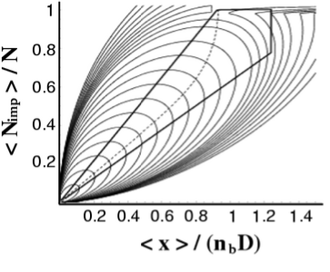
Figure 14: Contour plot of Landau free energy landscape as a function of two independent variables $\Phi(x,N_{\rm imp})$. The corridor of the fully confined relaxed chain in the upper right corner is artificially broadened for a clearer visual picture. Also shown are the parametric trajectories $<N_{\rm imp}(t)>$ vs. $<x(t)>$ of the de-confinement process for two limiting cases $D_{x}<<D_{n}$ and $D_{x}>>D_{n}$ (solid lines) and for isotropic diffusion $D_{x}=D_{n}$ (dashed line).

A contour plot showing the landscape of $\Phi(x,N_{\rm imp})$ is presented in Figure 14. States corresponding to a fully confined relaxed chain are depicted by a narrow corridor in the upper right part of the landscape. The lower left corner represents a completely free chain with the lowest possible free energy. The corridor is generally separated from the sloping landscape by a barrier, except for an opening in the vicinity of $x=x_{\rm sp}^{(1)}$.

Full dynamic evolution in the $(x,N_{\rm imp})$ configuration space will be governed by a Fokker-Planck equation with Landau free energy playing the role of effective potential. However, if one avoids the detailed description of barrier-crossing events, the problem is simplified considerably. The dynamics of averaged quantities $<x(t)>$ and $<N_{\rm imp}(t)>$ is then driven by thermodynamic forces $\frac{\partial\Phi(x,N_{\rm imp})}{\partial x}$ and $\frac{\partial\Phi(x,N_{\rm imp})}{\partial N_{\rm imp}}$, respectively, and the coupled non-linear equations of motion are given as

$$\frac{d<x(t)>}{dt}=-D_{x}\frac{\partial\Phi}{\partial x}$$ (26)

and

$$\frac{d<N_{\rm imp}(t)>}{dt}=-D_{n}\frac{\partial\Phi}{\partial N_{\rm imp}}$$ (27)

where $D_{x}$ and $D_{n}$ are the effective diffusion coefficients along the $x$ and $N_{\rm imp}$ coordinates, correspondingly. Geometrically, this evolution is a diffusive slide along the slopes of the Landau free energy in a two-dimensional configuration space. A detailed discussion of the diffusion coefficients and the physics behind them is well beyond the scope of this paper.

Here we briefly present the result of a dynamic analysis for three different scenarios. First we analyze the two limiting cases discussed in Section 8. Equations of motion were solved numerically for very slow $x$ dynamics with $D_{x}=10^{-3}D_{n}$ and the curve of $<N_{\rm imp}(t)>$ vs. $<x(t)>$ parametrically defined by $t$ is shown in Figure 14. It is clear that this coincides with the quasi-static trajectory predicted in the $x$-ensemble. Another curve was obtained from a numerical solution assuming slow $N_{\rm imp}$ dynamics with $D_{n}=10^{-3}D_{x}$. This coincides precisely with the $N_{\rm imp}$-ensemble description as evidenced by comparing Figures 13 and 14. Finally, the parametric curve for the case of isotropic diffusion $D_{x}=D_{n}$ is also presented. This is characterized by a relatively rapid initial growth of the ejected part of the chain, the distant end position evolution catching up with some delay. Eventually, the trajectory slide down the valley along its geometrical bottom line. The shapes of all three trajectories are insensitive to assumptions made about the change in diffusion coefficients during the de-confinement process as long as their ratio is kept fixed.

References

- (1) Salman, H.; Zbaida, D.; Rabin, Y.; Chatenay, D.; Elbaum, M. Proc. Natl. Acad. Sci. U.S.A. 2001, 98, 7247.
- (2) Meller, A. J. Phys.: Condens. Matter 2003, 15, R581.
- (3) Kasianowicz, J. J.; Brandin, E.; Branton, D.; Deaner, D. W. Proc. Natl. Acad. Sci. U.S.A. 1996, 93, 13770.
- (4) Aktson, M.; Branton, D.; Kasianowicz, J. J.; Brandin, E.; Deaner, D. W. Biophys. J. 1999, 77, 3227.
- (5) Meller, A.; Nivon, L.; Brandin, E.; Golovchenko, J. A.; Branton, D. Proc. Natl. Acad. Sci. U.S.A. 2000, 97, 1079.
- (6) Clausen-Schaumann, H.; Seitz, M.; Krautbauer R.; Gaub, H. E. Curr. Opin. Chem. Biol. 2001, 4, 524.
- (7) Williams, M. C.; Rouzina, I. Curr. Opin. Struct. Biol. 2002, 12, 330.
- (8) Reisner, W.; Morton, K. J.; Riehn, R.; Wang, Y. M.; Yu, Z.; Rosen, M.; Sturm, J. C.; Chou, S. Y.; Frey, E.; Austin, R. H. Phys. Rev. Lett. 2005, 94, 196101.
- (9) Grassberger, P. Phys. Rev. E 1997, 56, 3682.
- (10) Hsu, H.-P.; Grassberger, P. Eur. Phys. J. 2003, B36, 209.
- (11) Hsu, H.-P.; Grassberger, P. J. Chem. Phys. 2004, 120, 2034.
- (12) Hsu, H.-P.; Binder, K.; Skvortsov, A. M.; Klushin, L. I. Phys. Rev. E 2007, 76 021108.
- (13) Sotta, P.; Lesne, A.; Victor, J. M. J. Chem. Phys. 2000, 112, 1565.
- (14) Kremer, K.; Binder, K. J. Chem. Phys. 1984, 81, 6381.
- (15) Milchev, A.; Paul, W.; Binder, K. Macromol. Theory Simul. 1994, 3, 305.
- (16) Yang, Y.; Burkhardt, T. M.; Gompper, G. Phys. Rev. E 2007, 76, 011804.
- (17) Daoud, M.; de Gennes, P. G. J. Phys. (paris) 1977, 38, 85.
- (18) Randel, R.; Loebl, H.; Matthai, C. Macromol. Theory Simul. 2004, 13, 387.
- (19) Subramanian, G.; Williams, D. R. M.; Pincus, P. A. Europhys. Lett. 1995, 29, 285; Macromolecules 1996, 29, 4045.
- (20) Ennis, J.; Sevick, E. M.; Williams, D. R. M. Phys. Rev. E 1999, 60, 6906.
- (21) Sevick, E. M.; Williams, D. R. M. Macromolecules 1999, 32, 6841.
- (22) Steels, B. M.; Leermakers, F. A. M.; Haynes, C. A. J. Chrom. B. 2000, 743, 31.
- (23) Milchev, A.; Yamakov, V.; Binder, K. Phys. Chem. Chem. Phys. 1999, 1, 2083; Europhys. Lett. 1999, 47, 675.
- (24) des Cloizeaux, J. J. Phys. (Paris) 1980, 41, 223.
- (25) Pincus, P. Macromolecules 1976, 9, 386.
- (26) Dimitrov, D. I.; Milchev, A.; Binder, K.; Klushin, L. I.; Skvortsov, A. M. e-print arXiv:0802.3116v1 2008.