Statistics of work performed on a forced quantum oscillator

Abstract

Various aspects of the statistics of work performed by an external classical force on a quantum mechanical system are elucidated for a driven harmonic oscillator. In this special case two parameters are introduced that are sufficient to completely characterize the force protocol. Explicit results for the characteristic function of work and the respective probability distribution are provided and discussed for three different types of initial states of the oscillator: microcanonical, canonical and coherent states. Depending on the choice of the initial state the probability distributions of the performed work may grossly differ. This result in particular holds also true for identical force protocols. General fluctuation and work theorems holding for microcanonical and canonical initial states are confirmed.

I Introduction

During the last decade various fluctuation and work theorems fwt ; ECM have been formulated and discussed. They inter alia characterize the full nonlinear response of a system under the action of a time dependent force J ; J07 . These theorems have been derived and experimentally confirmed primarily for classical systems ex ; BLR ; BHSB . Quantum mechanical generalizations were proposed recently qm ; M ; RM ; EM ; TLH ; TH ; TMH ; DL .

Conceptual problems though arise in the context of quantum mechanics if one tries to generalize those classical relations that require for example the specification of a system’s trajectory extending over some interval of time, or the simultaneous measurement of noncommuting observables. For example, the measurement of work performed by an external force on an otherwise isolated system may be accomplished in the framework of classical physics in principle in two different ways. The first method is based on two measurements of the energy, one at the beginning and the second at the end of the considered process. This method becomes unreliable in practice if the system is large and the work performed on the system is negligibly small compared to the total energy of the system. Such a situation typically arises if the system of interest, on which the force exclusively acts, interacts with its environment. In order to retain an isolated system, the large system made of the open system and its environment must be considered. Again, the work performed on the system results as the difference of the energies of the total system, which both may be very large.

For classical systems, this unfortunate situation can be circumvented by a second method, by monitoring the state of the relevant small system during the time when the force is acting. Having this information at hand one can determine the work by integrating the power supplied to the system at each instant of time. The respective power can be inferred from the registered state of the system and the known force protocol. In a quantum system a continuous measurement of even a single observable would strongly influence and possibly manifestly distort the system’s dynamics. Apparently, only the first method of two energy measurements is feasible, at least in principle, in the quantum context.

An alternative method based on a continuous monitoring has recently been suggested by Esposito and Mukamel EM for open quantum systems described by Markovian quantum master equations. There the dynamics of the density matrix is mapped onto a classical rate process for which known fluctuation theorems can be applied Seif . This provides an interesting formal approach but its physical meaning has remained unclear EM . Moreover, this approach is restricted to open systems that only weakly interact with their respective environments.

In the present paper the distribution of work is discussed for the exactly solvable system of a driven harmonic oscillator DL ; H . In this case, the distribution of work is discrete. We provide formal expressions for this distribution and its corresponding characteristic function which are valid for all initial states of the system as well as for all possible kinds of force protocols. In particular, we determine the characteristic functions and distributions of the work for microcanonical, canonical and coherent initial states which lead to qualitatively different work distributions.

The paper is organized as follows. In Sect. II we review the general form of the characteristic function of work performed on a system in terms of a correlation function of the exponentiated Hamiltonians at the initial and final time of the force protocol. We prove that this particular expression indeed always represents a characteristic function, i.e. the Fourier transform of a probability density. Sect. III presents various fluctuation and work theorems for canonical and microcanonical initial states. In Sect. IV general expressions for the characteristic function and the corresponding probability distribution of work are derived for a driven harmonic oscillator. Moreover, the expressions for the first four cumulants are derived. The dependence of the work distribution on the force protocol for microcanonical, canonical and coherent initial states as well as its dependence on the specific parameters of these initial states are investigated.

II Characteristic function of work

The response of a quantum system on a perturbation by a classical, external force can be characterized by the change of energies contained in the total system. The energy as an observable coincides with its Hamiltonian $H(t)$ of the total system. It includes the external force and therefore depends on time. We will consider the dynamics of the system only within a finite window of time $[t_{0},t_{f}]$ during which the force is acting in a prescribed way, resulting in a protocol of Hamiltonians which is denoted by $\{H(t)\}_{t_{f},t_{0}}$. Apart from the action of the external force the system is assumed to be closed. Its dynamics is consequently governed by a unitary time evolution $U_{t,t_{0}}$, which is the solution of the Schödinger equation

$$\begin{split}i\hbar\partial U_{t,t_{0}}/\partial t&=H(t)U_{t,t_{0}},\\ U(t,t_{0})&=1.\end{split}$$ (1)

As explained in the introduction, the work $w$ is measured as the difference of the energies of the system at the final and initial times $t_{f}$ and $t_{0}$. In a single measurement the work is given by the difference of two eigenvalues $e_{n}(t_{f})$ and $e_{m}(t_{0})$ of the Hamiltonians $H(t)$ at the respective times $t_{f}$ and $t_{0}$, i.e. by $w=e_{n}(t_{f})-e_{m}(t_{0})$. The inherent randomness of the outcome of a quantum measurement in general leads to a measured work that is random. A complete description of the statistical properties of the work performed on the system is provided by the characteristic function $G_{t_{0},t_{f}}(u)$ which presents the Fourier transform of the probability density of the work $p_{t_{f},t_{0}}(w)$, i.e.

$$G_{t_{0},t_{f}}(u)=\int dw\>e^{iuw}p_{t_{f},t_{0}}(w).$$ (2)

It can be expressed as a quantum correlation function of the exponentiated Hamiltonian at the initial and the final time TMH , i.e.

$$\begin{split}G_{t_{0},t_{f}}(u)&=\langle e^{iuH(t_{f})}e^{-iuH(t_{0})}\rangle\\ &\equiv\mbox{Tr}e^{iuH_{H}(t_{f})}e^{-iuH(t_{0})}\bar{\rho}(t_{0}),\end{split}$$ (3)

where

$$H_{H}(t_{f})=U^{+}_{t_{f},t_{0}}H(t_{f})U_{t_{f},t_{0}}$$ (4)

denotes the Hamiltonian in the Heisenberg picture. The density matrix $\bar{\rho}(t_{0})$ from the initial density matrix $\rho(t_{0})$ as a result of the measurement of the Hamiltonian $H(t_{0})$. It is given by

$$\bar{\rho}(t_{0})=\sum_{n}P_{n}(t_{0})\rho(t_{0})P_{n}(t_{0}),$$ (5)

where the operators $P_{n}(t_{0})$ denote the eigenprojection operators of the Hamiltonian at time $t_{0}$, which present a partition of the unity

$$\sum_{k}P_{n}(t_{0})=1.$$ (6)

Before we apply the general expression (3) to a particular system and investigate its dependence on the initial state $\rho(t_{0})$, we discuss three general properties of the correlation expression (3) which guarantee that the resulting function $G_{t_{f},t_{0}}(u)$ indeed always presents a proper characteristic function of a classical random variable $w$. This is the consequence of the three following properties:
(i) $G_{t_{f},t_{0}}(u)$ is a continuous function of $u$.
(ii) $G_{t_{f},t_{0}}(u)$ is a positive definite function of $u$, i.e. for all integer numbers $n$, all real sequences $u_{1},u_{2},\ldots u_{n}$, and all complex numbers $z_{i}$, $i=1,2\ldots n$

$$\sum_{i,i^{\prime}}^{n}G_{t_{f},t_{0}}(u_{i}-u_{i^{\prime}})z^{*}_{i}z_{i^{\prime}}\geq 0$$ (7)

holds. Here, the asterisk $z_{i}^{*}$ denotes the complex conjugate of $z_{i}$.
(iii) $G_{t_{f},t_{0}}(0)=1$
According to a theorem by Bochner Boch the properties (i-iii) are necessary and sufficient conditions in order that the function $G_{t_{f},t_{0}}(u)$ is the Fourier transform of the probability measure of a random variable. In short, the first condition insures that, strictly speaking, the function $G_{t_{f},t_{0}}(u)$ is the Fourier transform of a measure, the second condition assures that this measure is positive and the third condition that it is normalized. Hence the correlation expression eq. (3) always defines a proper characteristic function. For a proof of the properties (i-iii) we refer the reader to the appendix A.

III Canonical and microcanonical initial states

In experiments an external force is often applied on a system that initially is found in a thermodynamic equilibrium state. Depending on whether the system was in weak contact with a heat bath or was totally isolated from its environment, the initial state of the system is described either by a canonical or a microcanonical density matrix. For both situations fluctuation and work theorems are known. We will shortly review these relations.

III.1 Work and fluctuation theorems for canonical initial states

If the initial density matrix is canonical, i.e. if

$$\rho(t_{0})=Z^{-1}(t_{0})\exp\{-\beta H(t_{0})\},$$ (8)

where

$$Z(t_{0})=\mbox{Tr}\exp\{-\beta H(t_{0})\}=e^{-\beta F(t_{0})}$$ (9)

denotes the partition function and $F(t_{0})$ the free energy, then $[H(t_{0}),\rho(t_{0})]=0$ and the first measurement of the energy leaves the density matrix unchanged, such that $\bar{\rho}(t_{0})=\rho(t_{0})$. With eq. (3) this leads to the characteristic function of work for a canonical initial state which was derived in Ref. TLH . In this case, $G_{t_{f},t_{0}}(u)$ can be continued to an analytic function of $u$ for all $0\leq\Im u\leq\beta$ TH . For the particular value $u=i\beta$ the characteristic function yields the mean value of the exponentiated work, $\langle\exp\{-\beta w\}\rangle$ and the correlation function expression (3) simplifies to the ratio of the partition functions at the times $t_{f}$ and $t_{0}$, resulting in the Jarzynski work theorem

$$\langle e^{-\beta w}\rangle=Z(t_{f})/Z(t_{0})=\exp\left\{-\beta(F(t_{f})-F(t_{0}))\right\},$$ (10)

where $Z(t_{f})=\text{tr}\exp\{-\beta H(t_{f})\}=\exp\{-\beta F(t_{f})\}$.

Within the domain of analyticity $\mathcal{S}=\{u|0\leq\Im u\leq\beta\}$ the characteristic functions for the original and the time reversed protocol are related to each other by the following formula, cf. TH

$$G_{t_{f},t_{0}}(u)=\frac{Z(t_{f})}{Z(t_{0})}G_{t_{0},t_{f}}(-u+i\beta),$$ (11)

where $G_{t_{0},t_{f}}(u)$ refers to processes under the time reversed protocol $\{H(t)\}_{t_{o},t_{f}}$ starting from the canonical state $Z^{-1}(t_{f})\exp\{-\beta H(t_{f})\}$. An inverse Fourier transform leads to the Tasaki-Crooks fluctuation theorem, which relates the probability densities of work $p_{t_{f},t_{0}}(w)$ for a given protocol to the density of the work $p_{t_{0},t_{f}}(w)$ for the time reversed protocol. This theorem explicitly reads TH

$$\frac{p_{t_{f},t_{0}}(w)}{p_{t_{0},t_{f}}(-w)}=\frac{Z(t_{f})}{Z(t_{0})}e^{\beta w}=e^{-\beta(F(t_{f})-F(t_{0})-w)}.$$ (12)

III.2 Fluctuation theorems for microcanonical initial states

A system in a microcanonical state is described by the density matrix

$$\rho(t_{0})=\varpi_{E}^{-1}(t_{0})\delta(H(t_{0})-E),$$ (13)

where

$$\varpi_{E}(t_{0})=\mbox{Tr}\>\delta(H(t_{0})-E)=\exp\left\{S(E,t_{0})/k_{B}\right\}$$ (14)

denotes the density of states as a function of the energy $E$ of the system. The density of states can be expressed in terms of the entropy of the system $S_{E}(t_{0})$ provided the spectrum of the system Hamiltonian is sufficiently dense such that the density of states becomes a smooth function on a coarsened energy scale. The microcanonical density matrix commutes with the Hamiltonian $H(t_{0})$. Consequently, $\bar{\rho}(t_{0})$ and $\rho(t_{0})$ coincide.

The microcanonical quantum Crooks theorem assumes the form TMH

$$\begin{split}\frac{p_{t_{f},t_{0}}(E,w)}{p_{t_{0},t_{f}}(E+w,-w)}&=\frac{\varpi_{E+w}(t_{f})}{\varpi_{E}(t_{0})}\\ &=\exp\left\{\frac{S(E+w,t_{f})-S(E,t_{0})}{k_{B}}\right\}.\end{split}$$ (15)

Analogous to the canonical case it relates the probability density $p_{t_{0},t_{0}}(E,w)$ of work $w$, for a system starting in a microcanonical state with energy $E$, to the respective quantity for the time reversed process starting at energy $E+w$. This quantum theorem is formally identical to the respective classical theorem CBK .

From the microcanonical Crooks theorem the probability density relating to the time reversed process can be eliminated to yield the so-called entropy-from-work theorem TMH , reading:

$$\varpi_{E_{f}}(t_{f})=\int dw\>\varpi_{E_{f}-w}(t_{0})p_{t_{f},t_{0}}(E_{f}-w,w)\;.$$ (16)

This theorem allows one to determine the unknown density of states of a system with Hamiltonian $H(t_{f})$ from the known density of states of a reference system $H(t_{0})$ by means of the statistics of the work that is performed on the system in a process that leads from the reference system to the final system with unknown density of states. In the case of systems with a sufficiently smooth density of states the respective entropy can be determined. For further details see in Ref. TMH .

IV Driven harmonic oscillator

To illustrate these concepts we consider an example which allows the analytical construction of the probability of work. Specifically we consider a harmonic oscillator on which a time dependent force acts during a finite interval of time. Its time evolution is governed by the Hamiltonian

$$H(t)=\hbar\omega a^{+}a+f^{*}(t)a+f(t)a^{+},$$ (17)

where $\omega$ denotes the angular frequency, and $a^{+}$ and $a$ creation and annihilation operators, respectively, which obey the usual commutation relation, i.e. $[a,a^{+}]=1$. The complex driving force $f(t)$ allows for a coupling to position and/or momentum of the oscillator. We assume that $f(t)$ vanishes for times $t\leq t_{0}=0$. It is our aim to study the influence of the initial state $\rho(t_{0})$ on the statistics of work performed on the oscillator. The measurement of $H(t_{0})=\hbar\omega a^{+}a$ at time $t_{0}=0$ then yields the result $\hbar\omega n$ with probability

$$p_{n}=\langle n|\rho(t_{0})|n\rangle.$$ (18)

Accordingly, the oscillator is found in the state

$$\bar{\rho}(t_{0})=\sum_{n}p_{n}|n\rangle\langle n|$$ (19)

immediately after this measurement. Putting this density matrix in the general expression for the characteristic function, eq. (3) one obtains

$$G_{t_{f},t_{0}}(u)=\sum_{n}p_{n}e^{-iu\hbar\omega n}\langle n|e^{iuH_{H}(t_{f})}|n\rangle\;.$$ (20)

For the driven harmonic oscillator the diagonal matrix element of the exponentiated Hamiltonian $H_{H}(t_{f})$ can be determined H . For details see the Appendix B. With the expression (60) for the matrix element $\langle n|\exp\left\{iH_{H}(t_{f})\right\}|n\rangle$ we find

$$\begin{split}G_{t_{f},t_{0}}(u)=&\>e^{iu|f(t_{f})|^{2}/(\hbar\omega)}\exp\left\{\left(e^{iu\hbar\omega}-1\right)|z|^{2}\right\}\sum_{n=0}^{\infty}\sum_{k=0}^{n}p_{n}\binom{n}{k}\frac{|z|^{2(n-k)}}{(n-k)!}e^{-iu\hbar\omega(n-k)}\left(e^{iu\hbar\omega}-1\right)^{2(n-k)}\\ &=\>e^{iu|f(t_{f})|^{2}/(\hbar\omega)}\exp\left\{\left(e^{iu\hbar\omega}-1\right)|z|^{2}\right\}\sum_{n=0}^{\infty}p_{n}L_{n}\!\left(4|z|^{2}\sin^{2}\frac{\hbar\omega u}{2}\right)\;,\end{split}$$ (21)

where $|f(t_{f})|^{2}/(\hbar\omega)$ denotes a uniform shift of the spectrum of the harmonic oscillator due to the presence of the external force, cf. eq. (55), and

$$z=\frac{1}{\hbar\omega}\int_{0}^{t_{f}}ds\dot{f}(s)\exp\{i\omega s\}$$ (22)

is a dimensionless functional of the driving force $f(t)$, cf. eq. (53). This dimensionless quantity vanishes in particular for all-quasi static forcings, i.e. if the force changes only very slowly with $f(t)=g(t/t_{f})$ for $t_{f}\to\infty$, where $g(\tau)$ is a continuously differentiable function for $\tau\in[0,1]$. We hence call $z(t)$ the rapidity parameter of the force protocol. Finally, $L_{n}(x)=\sum_{k=0}^{n}\binom{n}{k}(-x)^{k}/k!$ denotes the Laguerre polynomial of order $n$ RG .

Introducing the cumulant generating function $K(u)=\ln G(u)$ one obtains the cumulants of work $k_{n}$ as the $n$th derivatives of $K(u)$ with respect to $u$ taken at $u=0$ vK , i.e. $k_{n}=(-i)^{n}d^{n}K(0)/du^{n}$. The first four cumulants become:

$$k_{1} =\langle w\rangle$$

$$=\frac{|f(t_{f})|^{2}}{\hbar\omega}+\hbar\omega|z|^{2},$$ (23)

$$k_{2} =\langle w^{2}\rangle-\langle w\rangle^{2}$$

$$=2(\hbar\omega)^{2}|z|^{2}\left(\langle a^{+}a\rangle_{0}+\frac{1}{2}\right),$$ (24)

$$k_{3} =\langle w^{3}\rangle-3\langle w^{2}\rangle\langle w\rangle+2\langle w\rangle^{3}$$

$$=\left(\hbar\omega\right)^{3}|z|^{2},$$ (25)

$$k_{4} =\langle w^{4}\rangle-4\langle w^{3}\rangle\langle w\rangle-3\langle w^{2}\rangle^{2}$$

$$\quad+12\langle w^{2}\rangle\langle w\rangle^{2}-6\langle w\rangle^{4}$$

$$=\left(\hbar\omega\right)^{4}|z|^{2}\left\{1+4\langle a^{+}a\rangle_{0}+6\left[\langle a^{+}a(a^{+}a-1)\rangle_{0}\right.\right.$$

$$\left.\left.\quad-2\langle a^{+}a\rangle_{0}\right]|z|^{2}\right\}.$$ (26)

The odd cumulants of the work are independent of the initial preparation. The even cumulants depend on the factorial moments of the number operator $a^{+}a$ with respect to the initial state $\bar{\rho}(t_{0})$ such as $\langle a^{+}a\rangle_{0}=\sum_{n}np_{n}$ and $\langle a^{+}a(a^{+}a-1)\rangle_{0}=\sum_{n}n(n-1)p_{n}$, where $p_{n}$ is defined in eq. (18). Moreover, all cumulants apart from the first one vanish for forcings with $z=0$. This holds true in particular for all quasi-static force characteristics. The underlying work probability density then shrinks to a delta function at $w=|f(t_{f})|^{2}/(\hbar\omega)$.

In general, the work probability density follows from the characteristic function by means of an inverse Fourier transformation. Rather than the characteristic function itself we first consider the function $\mathcal{G}(u)\equiv\exp\left\{-iu|f(t_{f})|^{2}/(\hbar\omega)\right\}G_{t_{f},t_{0}}(u)$. Upon expanding $\exp\left\{|z|^{2}\exp\left\{iu\hbar\omega\right\}\right\}$ into a series of powers of $|z|^{2}$ we obtain for $\mathcal{G}(u)$ a Laurent series in the variable $\exp\left\{iu\hbar\omega\right\}$. The inverse Fourier transformation is given by a series of delta functions $\delta(w-\hbar\omega r)$, with $r\in\mathbb{Z}$, with weights

$$\begin{split}q_{r}=&e^{-|z|^{2}}\sum_{m,n=0}^{\infty}\sum_{k=0}^{n}\sum_{l=0}^{2k}(-1)^{2k-l}p_{n}\\ &\quad\times\frac{|z|^{2(k+m)}}{m!\>k!}\binom{n}{k}\binom{2k}{l}\delta_{l+m,k+r}\\ =&e^{-|z|^{2}}\sum_{n=0}^{\infty}\sum_{k=0}^{n}\sum_{l=0}^{\text{min}(k+r,2k)}(-1)^{2k-l}p_{n}\\ &\quad\times\frac{|z|^{2(2k+r-l)}}{(k+r-l)!\>k!}\binom{n}{k}\binom{2k}{l}\;.\end{split}$$ (27)

The factor $\exp\left\{-iu|f(t_{f})|^{2}/(\hbar\omega)\right\}$, by which $\mathcal{G}(u)$ has to be multiplied to yield $G_{t_{f},t_{0}}(u)$, gives rise to a constant shift such that the probability density of work performed on a harmonic oscillator assumes the result

$$p_{t_{f},0}(w)=\sum_{r}q_{r}\>\delta\!\left(w-(\hbar\omega r+\frac{|f(t_{f})|^{2}}{\hbar\omega})\right)\;.$$ (28)

In the next Section we will investigate the influence of the initial state on the statistics of the work.

IV.1 Distributions of work for different initial states

As particular examples of initial states we will discuss microcanonical, canonical and coherent states.

IV.1.1 Microcanonical initial state

For a microcanonical initial state with energy $\hbar\omega n_{0}$ the density matrix becomes

$$\rho(t_{0})=\bar{\rho}(t_{0})=|n_{0}\rangle\langle n_{0}|.$$ (29)

The characteristic function then reads

$$\begin{split}G^{\text{mc}}_{t_{f},t_{0}}(n_{0},u)&=e^{iu|f(t_{f})|^{2}/(\hbar\omega)}\exp\left\{\left(e^{iu\hbar\omega}-1\right)|z|^{2}\right\}\\ &\quad\times L_{n_{0}}\!\left(4|z|^{2}\sin^{2}\frac{\hbar\omega u}{2}\right)\end{split}$$ (30)

and, accordingly, the probability $q^{\text{mc}}_{r}(n_{0})$ to find a change of energy by $w=\hbar\omega r+|f(t_{f})|^{2}/(\hbar\omega)$ emerges as

$$\begin{split}q^{\text{mc}}_{r}(n_{0})&=e^{-|z|^{2}}\sum_{k=0}^{n_{0}}\sum_{l=0}^{\min(k+r,2k)}\frac{(-1)^{2k-l}}{(k+r-l)!\>k!}\\ &\quad\times\binom{n}{k}\binom{2k}{l}|z|^{2(2k+r-l)}.\end{split}$$ (31)

As expected from the behavior of the moments, all probabilities $q^{\text{mc}}_{r}(n_{0})$ with $r\neq 0$ vanish for quasi-static forcing, i.e. if $z\to 0$. The dependence of $q^{\text{mc}}_{r}(n_{0})$ for $n_{0}=0$ and $3$ as well as for the eight lowest values of $r$ on the parameter $z$ is displayed in Fig. 1. With increasing values of the rapidity parameter $z$ the distribution is becoming broader.

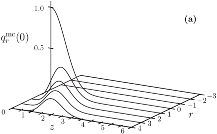
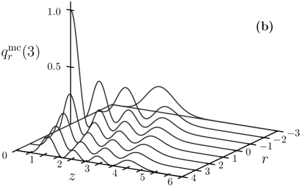
Figure 1: The probabilities $q^{\text{mc}}_{r}(n_{0})$ for two microcanonical initial states with $n_{0}=0$ (a) and $n_{0}=3$ (b) are depicted for $r=-3\ldots 4$, as functions of the rapidity parameter $z$ in eq. (53). In both cases the distribution collapses at $r=0$ for adiabatic forcing corresponding to $|z|=0$ and broadens with increasing $|z|$. Obviously, when starting in the ground state the oscillator cannot deliver work whence the probability for negative $r$ strictly vanishes. “Stimulated emission” becomes possible from an excited state at finite driving rapidity $z$ leading to nonzero probabilities $q^{\text{mc}}_{r}(n_{0})$ at negative values of $r$ in panel (b).

For the fixed value of $|z|=2$ the distribution $q^{\text{mc}}_{r}(n_{0})$ is compared for the three initial states with $n_{0}=0$ , $10$ and $30$ in Fig. 2.

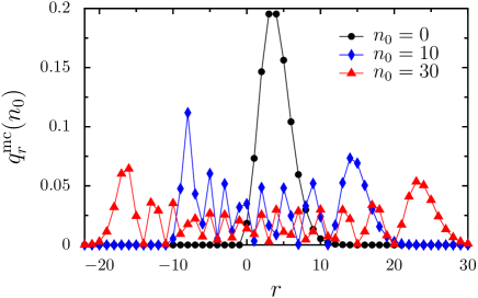
Figure 2: (Color online) The probabilities $q^{\text{mc}}_{r}(n_{0})$ for a microcanonical initial state with $n_{0}=0$ (circles) and $n_{0}=10$ (diamonds) and $n_{0}=30$ (crosses) are compared for a fixed rapidity parameter $|z|=2$ and $r=-22\ldots 30$. The lines serve as a guide for the eye.

With increasing value of $n_{0}$ the distributions become broader. They develop a slightly asymmetric shape with higher peaks at negative values of $r$ compared to those at positive $r$ values. Between these dominant peaks the probability still displays pronounced variations.
For a harmonic oscillator, the microcanonical Crooks theorem reduces to the relation $q^{\text{mc}}_{r}(n)=q^{\text{mc}}_{-r}(n+r)$. One can show that this symmetry is fulfilled by the probabilities $q^{\text{mc}}_{r}(n)$ given by eq. (31).

IV.1.2 Canonical initial state

For a canonical density matrix

$$\rho(t_{0})=(1-e^{-\beta\hbar\omega})e^{-\beta\hbar\omega a^{+}a}$$ (32)

the initial states are distributed according to $p_{n}=e^{-\beta\hbar\omega n}/(1-e^{-\beta\hbar\omega})$. This allows one to perform the sum over $n$ in the expression for the characteristic function (21) in terms of the generating function of the Laguerre polynomials, cf. RG yielding the expression

$$G^{\text{c}}_{t_{f},t_{0}}(\beta,u)=\exp\left\{\frac{iu|f(t_{f})|^{2}}{\hbar\omega}+\left(e^{iu\hbar\omega}-1\right)|z|^{2}-4|z|^{2}\frac{\sin^{2}(\hbar\omega u/2)}{e^{\beta\hbar\omega}-1}\right\}.$$ (33)

Putting $u=i\beta$ one finds that the two terms in the exponent which are proportional to $|z|^{2}$ cancel each other, such that one obtains

$$\langle e^{\beta w}\rangle=G^{\text{c}}_{t_{f},t_{0}}(\beta,i\beta)=\exp\left\{-\beta|f(t_{f}|^{2}/(\hbar\omega)\right\}.$$ (34)

The free energy difference of two oscillators with Hamiltonians $H(t_{0})=\hbar\omega a^{+}a$ and $H(t_{f})=\hbar\omega a^{+}a+f^{*}(t_{f})a+f(t)a^{+})$ each one staying in a canonical state at the temperature $\beta$ is given by $\Delta F=F(t_{f})-F(t_{0})=|f(t_{f})|^{2}/(\hbar\omega)$ in accordance with Jarzynski’s work theorem.

The probability $q^{\text{c}}_{r}(\tilde{\beta})$ to find the work $w=\hbar\omega r+|f(t_{f})|^{2}/(\hbar\omega)$ if the system starts in a canonical state becomes

$$\begin{split}q^{\text{c}}_{r}(\tilde{\beta})&=e^{-|z|^{2}}\left(1-e^{-\tilde{\beta}}\right)\sum_{n=0}^{\infty}\sum_{k=0}^{n}\sum_{l=0}^{\min(k+r,2k)}(-1)^{l}e^{-\tilde{\beta}n}\\ &\quad\times\frac{|z|^{2(2k+r-l)}}{(k+r-l)!k!}\binom{n}{k}\binom{2k}{l}\end{split}$$ (35)

where $\tilde{\beta}=\beta\hbar\omega$ denotes the inverse dimensionless temperature of the initial state. The expression for $q^{c}_{r}(\tilde{\beta})$ can be further simplified to read

$$q^{\text{c}}_{r}(\tilde{\beta})=e^{-|z|^{2}\coth(\tilde{\beta}/2)}e^{\tilde{\beta}r/2}I_{r}\left(\frac{|z|^{2}}{\sinh\tilde{\beta}/2}\right)$$ (36)

where $I_{\nu}(x)$ denotes the modified Bessel function of first kind of order $\nu$ RG . For details of the derivation see Appendix C.

Note that the following detailed balance like symmetry relation exists,

$$q^{\text{c}}_{-r}(\tilde{\beta})=e^{-\tilde{\beta}r}q^{\text{c}}_{r}(\tilde{\beta}),$$ (37)

relating the occurence of positive and negative work. In Fig. 3 the $z$ dependence of $q^{c}_{r}(\tilde{\beta})$ for $\tilde{\beta}=\ln(4/3)$ is compared for a few small values of $r$. One finds that due to the average over the canonical initial distribution the multipeaked structure of the microcanonical distribution as a function of the rapidity parameter $|z|$ disappears and only a single peak remains for each value of $r$. The temperature dependence of the work distribution is illustrated in Fig. 4.

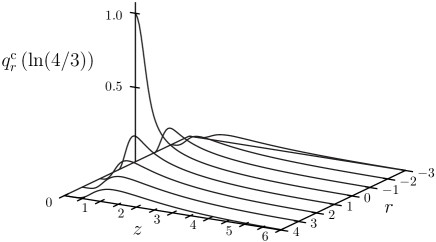
Figure 3: The probabilities $q^{\text{c}}_{r}(\tilde{\beta}=\ln(4/3))$ for a canonical initial state are displayed for $r=-3\ldots 4$ as a function of the parameter $z$. For the sake of comparability the dimensionless inverse temperature is chosen such that the average energy in the initial state coincides with the energy $3\hbar\omega$ of the microcanonical state in Fig. 1 (b).

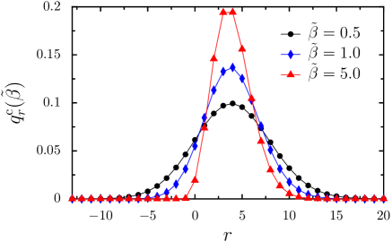
Figure 4: (Color online) The probabilities $q^{\text{c}}_{r}(\tilde{\beta})$ for a canonical initial state are displayed as functions of $r$ for $|z|=2$ and different values of the dimensionless inverse temperature $\tilde{\beta}=0.5$ (boxes), $1$ (circles) and $5$ (crosses). The lines serve as a guide for the eye.

Finally, we verify the validity of the Tasaki-Crooks theorem (12) for a driven oscillator. For this purpose we consider the probability density $p_{t_{0},t_{f}}(-w)$ for the time reversed protocol. Since the absolute values of the rapidity parameters coincide for the original and the time reversed protocol the probability density of work for the reversed protocols becomes

$$p_{t_{0},t_{f}}(-w)=\sum_{r=-\infty}^{\infty}q_{r}\delta\left(-w-(\hbar\omega r-\frac{|f(t_{f})|^{2}}{\hbar\omega})\right)\;,$$ (38)

where we took into account the overall shift of the spectrum by the reversed protocol as $-|f(t_{f})|/(\hbar\omega)$. Multiplying both sides of eq. (38) with $\exp\left\{-\beta(\Delta F-w)\right\}=\exp\left\{-\beta(|f(t_{f})|^{2}/(\hbar\omega)-w)\right\}$ one obtains

$$\begin{split}e^{-\beta(\Delta F-w)}p_{t_{0},t_{f}}(-w)&=\sum_{r}e^{-\beta\left(|f(t_{f})|^{2}/(\hbar\omega)-w\right)}q^{\text{c}}_{r}(\tilde{\beta})\\ &\quad\times\delta\left(-w-(\hbar\omega r-\frac{|f(t_{f})|^{2}}{\hbar\omega})\right)\\ &=\sum_{r}e^{\tilde{\beta}r}q^{c}_{r}(\beta)\\ &\quad\times\delta\left(w+(\hbar\omega r-\frac{|f(t_{f})|^{2}}{\hbar\omega})\right)\\ &=p_{t_{f},t_{0}}(w),\end{split}$$ (39)

in accordance with the Tasaki-Crooks theorem (12).

IV.1.3 Coherent initial state

An oscillator prepared in a coherent state $|\alpha\rangle$ is described by the density matrix

$$\rho(t_{0})=|\alpha\rangle\langle\alpha|$$ (40)

where

$$|\alpha\rangle=e^{\alpha a^{+}+\alpha a}|0\rangle$$ (41)

and $|0\rangle$ is the normalized ground state of the oscillator satisfying $a|0\rangle=0$. Note that the coherent state density matrix does not commute with the Hamiltonian $H(t_{0})$. The measurement of $H(t_{0})$ modifies the coherent state (40) by projecting it onto the eigenstates $|n\rangle=(a^{+})^{n}/\sqrt{n!}|0\rangle$ of this Hamiltonian leading to

$$\bar{\rho}(t_{0})=e^{-|\alpha|^{2}}\sum_{n}\frac{|\alpha|^{2n}}{n!}|n\rangle\langle n|$$ (42)

This implies a Poissonian distribution of the respective energy eigenvalues $\hbar\omega n$

$$p^{\text{cs}}_{n}=\frac{|\alpha|^{2n}}{n!}e^{-|\alpha|^{2}},$$ (43)

which yields for the characteristic function of work (21) a closed expression of the form

$$\begin{split}G^{\text{cs}}_{t_{f},t_{0}}(\alpha,u)&=\exp\left\{\frac{iu|f(t_{f})|^{2}}{\hbar\omega}+|z|^{2}\left(e^{i\hbar\omega u}-1\right)\right\}\\ &\quad\times J_{0}\left(4\left|\alpha z\sin\frac{\hbar\omega u}{2}\right|\right)\end{split}$$ (44)

where $J_{0}(x)$ is the Bessel function of order zero, cf. Ref. RG . For the probability $q^{\text{cs}}_{r}(\alpha)$ of work one obtains with eq. (27)

$$q^{\text{cs}}_{r}(\alpha)=\;e^{-|z|^{2}}\sum_{m=0}^{\infty}\frac{|z|^{2m}\>|\alpha z|^{2|m-r|}}{m!\left(|m-r|!\right)^{2}}{}_{1}F_{2}\left(|m-r|+\frac{1}{2};|m-r|+1,2|m-r|+1;-4|\alpha z|^{2}\right)$$ (45)

where ${}_{1}F_{2}(a;b,x;x)$ denotes a generalized hypergeometric function RG . For details of the derivation see the Appendix D.

The dependence of the probabilities $q^{\text{cs}}_{r}(\alpha)$ on the rapidity parameter $|z|$ is illustrated in Fig. 5 for $r$ values ranging from $-10$ to $20$.

Figure 5: The probabilities $q^{\text{cs}}_{r}(\alpha)$ for a coherent state with parameter $|\alpha|=3$ are displayed for $r=-10\ldots 20$ as functions of $z$.

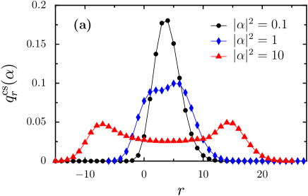
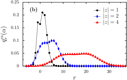
Figure 6: (Color online) The distribution of work performed on an oscillator which initially is prepared in a coherent state $|\alpha\rangle$ for different values of $\alpha$ in panel (a) and of the rapidity parameter $z$ in panel (b). In panel (a) the rapidity parameter has the value $|z|=2$. In panel (b) the coherent state parameter has the value $|\alpha|^{2}=1$.

Increasing values of $z$ lead to a broadening of the distribution and also to a shift towards larger values of $r$, see also panel (b) of Fig. 6. This is in accordance with eq. (23) and (24) for the first two cumulants of the work, which both increase with $|z|^{2}$. Panel (a) of Fig. 6 shows the dependence of the probabilities $q^{\text{cs}}_{r}(\alpha)$ on the parameters $\alpha$. Increasing $\alpha$ also leads to a broadening of the work distribution without influencing its mean value, cf. also eq. (23).

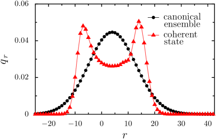
Figure 7: (color online) The distribution of work is compared for a canonical and a coherent initial state subject to the same force protocol with rapidity parameter $z=2$. With $\beta\hbar\omega=0.1$ and $|\alpha|^{2}\approx 9.51$ the expectation values of the energies agree in the two initial states such that according to eqs. (23) and (24) the first and second moments of the work also coincide. Still the distributions of work grossly differ from each other.

In Fig. 7 the probabilities $q_{r}$ are depicted for different initial states. In one case the oscillator is initially prepared in a canonical state at inverse dimensionless temperature $\tilde{\beta}=\beta\hbar\omega=0.1$. In the other case, the oscillator stays in a coherent state $|\alpha\rangle$, where the absolute value of $|\alpha|$ is chosen such that the mean excitation number is the same for both states, i.e. $|\alpha|^{2}=\exp\{-\beta\hbar\omega\}/(1-\exp\{-\beta\hbar\omega\})$. For $\beta\hbar\omega=0.1$ one finds $|\alpha|^{2}\approx 9.51$. The two oscillators then are subjected to protocols with the same rapidity parameter $|z|=2$. According to eqs. (23) and (24) the first two moments of the work performed on the oscillator coincide. Yet the distribution of weight factors $q^{\text{c}}_{r}(\tilde{\beta})$ and $q^{\text{cs}}_{r}(\alpha)$ distinctly differ. Whereas the distribution is pronouncedly bimodal in case of the coherent state, it is unimodal for the canonical state. The weight factors $q^{\text{c}}_{r}(\tilde{\beta})$ almost perfectly fall onto the Gaussian probability density which has the same first two moments as the discrete distribution given by $q_{r}$.

V Conclusions

In this work we studied the statistics of work performed on an externally driven quantum mechanical oscillator by means of a correlation function expression of the work. We demonstrated that this particular expression indeed always represents a proper characteristic function of a random variable, which is the performed work in the present context. The proof given here is based on Bochner’s theorem. It holds for general quantum mechanical systems, not only for harmonic oscillators.

The considered force linearly couples to the position and momentum of the oscillator. It may describe the influence of an electric field on charged particles in a parabolic trap or the external forcing of a single electromagnetic cavity mode. For this type of additive forcing, the frequency of the oscillator remains unchanged and therefore the level spacing of the eigenvalues of the Hamiltonian is not influenced by the force. The spectrum is only shifted as a whole. As a consequence the work performed on the oscillator is, as a positive or negative integer of the level spacing, a discrete random variable. We determined the first few cumulents of the work for arbitrary force protocols and initial states. A complementary study for a parametrically forced oscillator was recently performed by Deffner and Lutz DL .

It turns out that for the harmonic oscillator the statistics of work depends on the force protocol $\{f(t)\}_{t_{f},t_{0}}$ only through two real parameters, which are (i) the shift of the spectrum, given by $L(t_{f})=|f(t_{f})|^{2}/(\hbar\omega)$, and (ii) the absolute value of the dimensionless quantity $z=\int_{t_{0}}^{t_{f}}\dot{f}(s)\exp\{i\omega s\}$. This parameter vanishes for all quasi-static processes and therefore presents a measure of the rapidity of the force protocol. While the presence of $L(t_{f})$ only causes an overall shift of the possible values of the work, the rapidity parameter $|z|$ also influences its distribution. Typically, the distributions move towards larger values of work $w$ and become broader with increasing rapidity $|z|$.

We also demonstrated that different initial states of the system such as microcanonical, canonical or coherent states, have a large influence on the work statistics. We further note that two different initial density matrices with the same diagonal elements with respect to the energy eigenbasis of the Hamiltonian $H(t_{0})$ lead to identical work distributions even though the two density matrices may be very different in other respects. For example, the coherent pure state $|\alpha\rangle\langle\alpha|$ and the mixed state $\exp\{-|\alpha|^{2n}\}\sum_{n}|\alpha|^{2}/n!|n\rangle\langle n|$ cannot be distinguished by means of their respective work statistics. This statistics is also insensitive to the phase of a coherent state.

Appendix A Proof of the properties of $G_{t_{f},t_{0}}(u,v)$

We prove that the conditions of Bochner’s theorem are fulfilled, and consequently $G_{t_{f},t_{0}}(u)$ is a proper characteristic function.

Proof of property (i): $G_{t_{f},t_{0}}(u)$ is a continuous function of $u$. The Hamiltonian operators at the two times of measurement $t_{0}$ and $t_{f}$ are selfadjoint operators. According to the theorem of Stone Yosida , each of the exponential operators $\exp\left\{-iuH(t_{0})\right\}$ and $\exp\left\{iuH_{H}(t_{f})\right\}$ forms a strongly continuous one-parameter group of unitary operators with parameter $u$. As the trace of a product of two strongly continuous operator valued functions of $u$ with the density operator $\bar{\rho}(t_{0})$, which is a trace class operator and independent of $u$, the characteristic function (3) is a continuous function of $u$.

Proof of property (ii): $G_{t_{f},t_{0}}(u)$ is a positive definite function of $u$. Using the cyclic invariance of the trace and the fact that $H(t_{0})$ and $\bar{\rho}(t_{0})$ commute with each other, we can rewrite the left hand side of the inequality (7) as

$$\sum_{i,j}^{n}G_{t_{f},t_{0}}(u_{i}-u_{j})z^{*}_{i}z_{j}=\sum_{i,j}^{n}\mbox{Tr}\>e^{i(u_{i}-u_{j})H_{H}(t_{f})}\>e^{-i(u_{i}-u_{j})H(t_{0})}\bar{\rho}(t_{0})z_{i}^{*}z_{j}=\mbox{Tr}A^{+}A\>\bar{\rho}(t_{0})\geq 0\;,$$ (46)

where

$$A=\sum_{i}z_{i}^{n}e^{-iu_{i}H_{H}(t_{f})}e^{iu_{i}H(t_{0})}$$ (47)

is a bounded operator and $A^{+}$ its adjoint. The last inequality in (46) immediately follows with the positivity of $A^{+}A$ and of the density matrix $\bar{\rho}(t_{0})$.

Proof of property (iii): $G_{t_{f},t_{0}}(0)=1$. For $u=0$ the exponential operators $\exp\left\{-iuH(t_{0})\right\}$ and $\exp\left\{iuH_{H}(t_{f})\right\}$ become unity. The trace over the density matrix $\bar{\rho}(t_{0})$ reduces by means of eqs. (5), (6) to the trace of the initial density matrix $\rho(t_{0})$, which is one.

Appendix B The matrix element $\langle n|\exp\{iuH_{H}(t_{f})\}|n\rangle$

The total time rate of change of the Hamiltonian $H_{H}(t)$ coincides with its partial derivative with respect to the time which for the driven oscillator becomes, cf. eq. (17),

$$\frac{dH_{H}(t)}{dt}=\dot{f}^{*}(t)a_{H}(t)-\dot{f}(t)a^{+}_{H}(t),$$ (48)

where $a_{H}(t)$ and $a^{+}_{H}(t)$ denote annihilation and creation operators, respectively, in the Heisenberg picture, which are given by

$$\begin{split}a_{H}(t)&=e^{-i\omega t}a-\frac{i}{\hbar}\int_{0}^{t}dse^{-i\omega(t-s)}f(s)\\ a^{+}_{H}(t)&=e^{i\omega t}a^{+}+\frac{i}{\hbar}\int_{0}^{t}dse^{i\omega(t-s)}f^{*}(s)\end{split}$$ (49)

This yields for $H_{H}(t_{f})$

$$H_{H}(t_{f})=\hbar\omega a^{+}a+B^{*}(t_{f})a+B(t_{f})a^{+}+C(t),$$ (50)

where

$$\begin{split}B(t_{f})&=\int_{0}^{t_{f}}ds\dot{f}(s)e^{i\omega s}\\ C(t_{f})&=\frac{i}{\hbar}\int_{0}^{t_{f}}ds\int_{0}^{s}ds^{\prime}\left[\dot{f}(s)f^{*}(s^{\prime})e^{i\omega(s-s^{\prime})}\right.\\ &\quad\left.-\dot{f}^{*}(s)f(s^{\prime})e^{-i\omega(s-s^{\prime})}\right].\end{split}$$ (51)

The unitary operator

$$V=e^{za^{+}-z^{*}a}$$ (52)

with

$$z=\frac{B(t_{f})}{\hbar\omega}$$ (53)

transforms $H_{H}(t)$ into

$$VH_{H}(t_{f})V^{+}=\hbar\omega a^{+}a+L(t_{f}),$$ (54)

where

$$L(t_{f})=C(t_{f})-\frac{|B(t_{f})|^{2}}{\hbar\omega}=\frac{|f(t_{f})|^{2}}{\hbar\omega}.$$ (55)

Note that $V$ induces a shift of the creation and annihilation operators

$$\begin{split}VaV^{+}=a-z,\quad Va^{+}V^{+}=a^{+}-z^{*}\end{split}$$ (56)

and further note that, when acting on the groundstate $|0\rangle$ with $a|0\rangle=0$, the operator $V$ yields the coherent state $|z\rangle$, i.e.

$$V|0\rangle=|z\rangle.$$ (57)

One finds with these properties

$${\allowdisplaybreaks}\langle n|e^{iuH_{H}(t_{f})}|n\rangle =\frac{1}{n!}\langle z|(a-z)^{n}\allowdisplaybreaks$$

$$\quad\times e^{iu\hbar\omega a^{+}a+iuL(t_{f})}(a^{+}-z^{*})^{n}|z\rangle\allowdisplaybreaks$$

$$=\frac{1}{n!}e^{iuL(t_{f})}\frac{\partial^{2n}}{\partial x^{n}\partial y^{n}}\allowdisplaybreaks$$

$$\quad\langle z|e^{x(a-z)}e^{iu\hbar\omega a^{+}a}e^{y(a^{+}-z^{*})}|z\rangle|_{x=y=0}$$ (58)

Here we have introduced the auxiliary variables $x$ and $y$ which allow to represent the $n$th powers of shifted creation and annihilation operators by derivatives of respective order. The scalar function $e^{-i(xz+yz^{*})}$ can be taken out of the scalar product and the remaining operator can be brought into normal order. It then becomes Wi

$$\begin{split}e^{xa}e^{iu\hbar\omega a^{+}a}e^{ya^{+}}&=\mathcal{N}\left\{\exp\left[(e^{iu\hbar\omega}-1)a^{+}a\right.\right.\\ &\quad\left.\left.+e^{iu\hbar\omega}\left(xa+ya^{+}+xy\right)\right]\right\}\;,\end{split}$$ (59)

where under the normal ordering operator $\mathcal{N}$ all creation operators stand left of the annihilation operators. The matrix element with respect to the coherent state $|z\rangle$ can be read off, yielding,

$$\begin{split}\langle n|e^{iuH_{H}(t_{f})}|n\rangle=&\>\frac{1}{n!}e^{iuL(t_{f})}\exp\left\{\left(e^{iu\hbar\omega}-1\right)|z|^{2}\right\}\frac{\partial^{2n}}{\partial x^{n}\partial y^{n}}\exp\left\{\left(e^{iu\hbar\omega}-1\right)(xz+yz^{*})+e^{iu\hbar\omega}xy\right\}|_{x=y=0}\\ =&\>\frac{1}{n!}e^{iuL(t_{f})}\exp\left\{\left(e^{iu\hbar\omega}-1\right)|z|^{2}\right\}\frac{\partial^{n}}{\partial y^{n}}\left[\left(e^{iu\hbar\omega}-1\right)z+e^{iu\eta\omega}y\right]^{n}\exp\left\{\left(e^{iu\hbar\omega}-1\right)\left(|z|^{2}+yz^{*}\right)\right\}|_{y=0}\\ =&\>e^{iu|f(t_{f})|^{2}/(\hbar\omega)}\exp\left\{\left(e^{iu\hbar\omega}-1\right)|z|^{2}\right\}\sum_{k=0}^{n}\binom{n}{k}\frac{|z|^{2(n-k)}}{(n-k)!}e^{iu\hbar\omega k}\left(e^{iu\hbar\omega}-1\right)^{2(n-k)}\;.\end{split}$$ (60)

Appendix C Work distribution for a canonical initial state

To determine the expression (36) for the work distribution $q^{\text{c}}(\tilde{\beta})$ we start from the general expression given in the first line of eq. (27). Interchanging the summation over the indices $n$ and $k$ we obtain

$$q^{c}_{r}(\tilde{\beta}) =e^{-|z|^{2}}\sum_{m,k=0}^{\infty}\sum_{l=0}^{2k}(-1)^{l}\frac{|z|^{2(k+m)}}{m!\>k!}\binom{2k}{l}\allowdisplaybreaks$$

$$\quad\times\delta_{l+m,k+r}\sum_{n=k}^{\infty}\frac{e^{-\tilde{\beta}n}}{1-e^{-\tilde{\beta}}}\binom{n}{k}\allowdisplaybreaks$$

$$\stackrel{{\scriptstyle(1)}}{{=}}e^{-|z|^{2}}\sum_{m,k=0}^{\infty}\sum_{l=0}^{2k}(-1)^{l}\frac{|z|^{2(k+m)}}{m!\>k!}\binom{2k}{l}\allowdisplaybreaks$$

$$\quad\times\left(\frac{1}{e^{\tilde{\beta}}-1}\right)^{k}\delta_{l+m,k+r}\allowdisplaybreaks$$

$$\stackrel{{\scriptstyle(2)}}{{=}}(-1)^{r}e^{-|z|^{2}}\sum_{m=0}^{\infty}\frac{(-|z|^{2})^{m}}{m!}\allowdisplaybreaks$$

$$\quad\times\sum_{k=|m-r|}^{\infty}\frac{\left(-|z|^{2}/(e^{\tilde{\beta}}-1)\right)^{k}}{k!}\binom{2k}{k+r-m}\allowdisplaybreaks$$

$$\stackrel{{\scriptstyle(3)}}{{=}}(-1)^{r}e^{-|z|^{2}}\sum_{m=0}^{\infty}\frac{(-|z|^{2})^{m}}{m!}e^{-2|z|^{2}/(e^{\tilde{\beta}}-1)}\allowdisplaybreaks$$

$$\quad\times I_{|m-r|}\left(-\frac{2|z|^{2}}{e^{\tilde{\beta}}-1}\right)\allowdisplaybreaks$$

$$\stackrel{{\scriptstyle(4)}}{{=}}e^{-|z|^{2}\coth(\tilde{\beta}/2)}\sum_{m=0}^{\infty}\frac{|z|^{2m}}{m!}I_{|m-r|}\left(\frac{2|z|^{2}}{e^{\tilde{\beta}}-1}\right)\allowdisplaybreaks$$

$$\stackrel{{\scriptstyle(5)}}{{=}}e^{-|z|^{2}\coth(\tilde{\beta}/2)}\left\{\sum_{m=0}^{\infty}\frac{|z|^{2}}{m!}I_{r-m}\left(\frac{2|z|^{2}}{e^{\tilde{\beta}}-1}\right)\right.\allowdisplaybreaks$$

$$\quad\left.+\sum_{m=r+1}^{\infty}\frac{|z|^{2}}{m!}\left[I_{m-r}\left(\frac{2|z|^{2}}{e^{\tilde{\beta}}-1}\right)\right.\right.\allowdisplaybreaks$$

$$\left.\left.\quad-I_{r-m}\left(\frac{2|z|^{2}}{e^{\tilde{\beta}}-1}\right)\right]\right\}\allowdisplaybreaks$$

$$=e^{-|z|^{2}\coth(\tilde{\beta}/2)}e^{\tilde{\beta}r/2}I_{r}\left(\frac{|z|^{2}}{\sinh(\tilde{\beta}/2)}\right).$$ (61)

In the first step ($\stackrel{{\scriptstyle(1)}}{{=}}$) we performed the sum on $n$ according to

$$\sum_{n=k}^{\infty}\frac{x^{k}}{1-x}\binom{n}{k}=\left(\frac{x}{1-x}\right)^{k},$$ (62)

cf. Ref. PBM , 5.2.11.3. In the second step $\stackrel{{\scriptstyle(2)}}{{=}}$ the Kronecker delta is used to perform the sum over k. The third step $\stackrel{{\scriptstyle(3)}}{{=}}$ is based on the relation

$$\sum_{k=|l|}^{\infty}\frac{x^{k}}{k!}\binom{2k}{k+l}=e^{2x}I_{|l|}(2x)$$ (63)

valid for integer $l$. Here $I_{\nu}(x)$ denotes the modified Bessel function of the first kind of order $\nu$. With $I_{\nu}(-x)=(-1)^{\nu}I_{\nu}(x)$ where $\nu$ is an integer, we come to the right hand side of the equality $\stackrel{{\scriptstyle(4)}}{{=}}$. In the next step the sum on $m$ is rewritten. The term in the square brackets vanishes because $I_{\nu}(x)$ is an even function of the order $\nu$. The remaining sum can be performed by means of the identity

$$\sum_{k=0}^{\infty}\frac{t^{k}}{k!}I_{\nu-k}(x)=\left(\frac{2t}{x}+1\right)^{\nu/2}I_{\nu}\left(\sqrt{x^{2}+2tx}\right)\;,$$ (64)

cf. PBM 5.8.3.1. This leads to the final result given in eq. (36).

Appendix D Work distribution for a coherent initial state eq. (45)

Starting from eq. (27) we may proceed in an analogous way as in the case of a canonical initial state, cf. the Appendix C. According to eq. (43) a Poissonian average over the binomial $\binom{n}{k}$ has to be performed instead of the geometric average in the first step of eq. (61). This yields

$$\sum_{n=k}^{\infty}\frac{|\alpha|^{2}}{k!}e^{-|\alpha|^{2}}\binom{n}{k}=\frac{|\alpha|^{2k}}{k!}\;.$$ (65)

Next the Kronnecker delta is used to perform the sum over $l$ leaving one with two sums of which the inner one over k can be expressed in terms of a generalized hypergeometric function, RG , to become

$$\sum_{k=|m-r|}^{\infty}\frac{(-|\alpha z|^{2})^{k}}{(k!)^{2}}\binom{2k}{k+r-m}=\frac{(-|\alpha z|^{2})^{|m-r|}}{(|m-r|!)^{2}}\\ {}_{1}F_{2}\left(|m-r|+\frac{1}{2};|m-r|+1,2|m-r|+1;-4|\alpha z|^{2}\right)\;.$$ (66)

This immediately leads to the expression in eq. (45).

References

- (1) G.N. Bochkov, Yu.E. Kuzovlev, Sov. Phys. JETP 45, 125 (1977).
- (2) D.J. Evans, E.G.D. Cohen, G.P. Morriss, Phys. Rev. Lett. 71, 2401 (1993).
- (3) C. Jarzynski, Phys. Rev. Lett. 78, 2690 (1997).
- (4) C. Jarzynsky, C. R. Physique 8, 495 (2007).
- (5) F. Douarche, S. Ciliberto, A. Petrosyan, I. Rabbiosi, Europhys. Lett. 70, 593 (2005).
- (6) C. Bustamante, J. Liphardt, F. Ritort, Physics Today 58 (7), 43 (2005).
- (7) V. Blickle, T. Speck, L. Helden, U. Seifert, C. Bechinger, Phys. Rev. Lett. 96, 070603 (2006).
- (8) H. Tasaki, cond-mat/0009244.
- (9) S. Mukamel, Phys. Rev. Lett. 90, 170604 (2003).
- (10) W. De Roeck, C. Maes, Phys. Rev. E 69, 026115 (2004).
- (11) M. Esposito, S. Mukamel, Phys. Rev. E 73, 046129 (2006).
- (12) P. Talkner, E. Lutz, P. Hänggi, Phys. Rev. E 75, 050102(R) (2007).
- (13) P. Talkner, P. Hänggi, J. Phys. A 40, F569 (2007).
- (14) P. Talkner, M. Morillo, P. Hänggi, arXiv:0707.2307v2.
- (15) S. Deffner, E. Lutz, Phys. Rev. E 77, 021128 (2008).
- (16) U. Seifert, J. Phys. A: Math. Gen. 37, L517 (2004).
- (17) K. Husimi, Prog. Theor. Phys. 9, 381 (1953).
- (18) E. Lukacs, Characteristic Functions, Griffin, London, 1970.
- (19) B. Cleuren, C. Van den Broeck, R. Kawai, Phys. Rev. Lett. 96, 050601 (2006).
- (20) K. Yosida, Functional Analysis, Springer Verlag, Berlin, 1971.
- (21) L.S. Gradshteyn, I.M. Ryzhik, Table of Integrals, Series and Products, Academic Press, San Diego (2000).
- (22) N.G. van Kampen, Stochastic Processes in Physics and Chemistry, North Holland, Amsterdam, 1992.
- (23) R.M. Wilcox, J. Math. Phys. 8, 962 (1967).
- (24) A.P. Prudnikov, Yu.A. Brychkov, O.I. Marichev, Integrals and Series, Vol. 1, Gordon and Breach, New York, 1986.