Nonlinear spectroscopy of photons bound to one atom

Abstract

Optical nonlinearities typically require macroscopic media, thereby making their implementation at the quantum level an outstanding challenge. Here we demonstrate a nonlinearity for one atom enclosed by two highly reflecting mirrorsBerman (1994). We send laser light through the input mirror and record the light from the output mirror of the cavity. For weak laser intensity, we find the vacuum-Rabi resonancesBoca et al. (2004); Maunz et al. (2005); Puppe et al. (2007a); Wallraff et al. (2004); Reithmaier et al. (2004); Yoshie et al. (2004); Peter et al. (2005); Khitrova et al. (2006); Press et al. (2007); Hennessy et al. (2007). But for higher intensities, we find an additional resonanceCarmichael et al. (1994). It originates from the fact that the cavity can accommodate only an integer number of photons and that this photon number determines the characteristic frequencies of the coupled atom-cavity systemRempe et al. (1987); Brune et al. (1996); Schuster et al. (2007). We selectively excite such a frequency by depositing at once two photons into the system and find a transmission which increases with the laser intensity squared. The nonlinearity differs from classical saturation nonlinearitiesRempe et al. (1991); Lugiato and Narducci (1992); Srinivasan and Painter (2007); Englund et al. (2007) and is direct spectroscopic proof of the quantum nature of the atom-cavity system. It provides a photon-photon interaction by means of one atom, and constitutes a step towards a two-photon gateway or a single-photon transistorChang et al. (2007).

The quantum nonlinearity has its origin in the fact that under the condition of strong coupling a system composed of a single atom and a single cavity mode has properties which are distinctively different from those of the bare atom (without the cavity), or the bare cavity (without the atom), or just the sum of the two (Fig. 1a). In fact the composite system forms a new quantum entity, the so-called atom-cavity molecule, made of matter and light, with its own characteristic energy spectrum. This spectrum consists of an infinite ladder of pairs of states, the dressed states (Fig. 1b). The first doublet contains one quantum of energy and can be probed by laser spectroscopy. For weak probing, the resulting spectrum is independent of the laser intensity and has been dubbed the vacuum-Rabi or normal-mode spectrum, consisting of a pair of resonances symmetrically split around the bare atomic and cavity resonances. This spectrum has first been observed with atomic beamsBerman (1994), and has been explored recently with single dipole-trapped atomsBoca et al. (2004); Maunz et al. (2005); Puppe et al. (2007a). It constitutes a benchmark for strong atom-cavity coupling and is central to most cavity quantum electrodynamics (QED) experiments, including those outside atomic physicsWallraff et al. (2004); Reithmaier et al. (2004); Yoshie et al. (2004); Peter et al. (2005); Khitrova et al. (2006); Press et al. (2007); Hennessy et al. (2007). Notice that the normal-mode spectrum on its own can equally well be described classically, by linear dispersion theory or a coupled oscillator model (atomic dipole and cavity field).

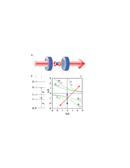
Figure 1: The atom-cavity molecule. (a) Artist’s conception of an atom enclosed by two cavity mirrors. The coupling of the atom to the intracavity light is so strong that the energy spectrum of the composite atom-cavity ‘molecule’ radically differs from the spectrum of its components. (b) Schematic of such a level structure illustrating how the dressed state $|2,-\rangle$ is directly accessed from the vacuum via a two-photon transition. (c) Location of the classical (normal-mode) resonances (dashed curves) and the first two quantum resonances (states $|2,\mp\rangle$ and $|3,\mp\rangle$) (solid curves). The diagonal arrow is the scan direction shown in Fig. 2, which crosses all resonances. A vertical scan along $\Delta_{a}=0$, as in Fig. 3, avoids the classical resonances. Resonances for the manifold ($n+1$) are located at $\Delta_{c}=\pm g/\sqrt{n}$ for $\Delta_{a}=0$.

The next higher lying doublet contains two quanta of energy and lacks a classical explanationCarmichael et al. (1994, 1996); Thompson et al. (1998). The corresponding dressed states have been observed (together with a few higher order states) in microwave cavity QEDRempe et al. (1987); Brune et al. (1996); Schuster et al. (2007) and even ion trapping, where phonons play the role of photonsMeekhof et al. (1996). At optical frequencies, evidence for these states has indirectly been obtained in two-photon correlation experiments where the conditional response of the system upon detection of an emitted photon is monitoredRempe et al. (1991); Mielke et al. (1998); Foster et al. (2000); Birnbaum et al. (2005). These optical experiments observe the quantum fluctuations in dissipative cavity QED systems but operate away from a resonance to a higher-lying state.

Our experiment exploits the anharmonicity of the energy-level spectrum to drive a multi-photon transition directly from the vacuum state to a specific higher lying state. We observe the quantum character of our cavity QED field by measuring a photon flux, not a photon correlation. To explain our technique, we note that a two-state atom coupled to a single-mode light field has a discrete spectrum consisting of a ladder of dressed states, $|n+1,\mp\rangle$, with frequencies

$$\omega_{n+1,\mp}\!=n\omega_{c}\!+\frac{1}{2}(\omega_{a}+\omega_{c})\mp\frac{1}{2}\sqrt{4g^{2}(n\!+1)+(\omega_{a}\!-\omega_{c})^{2}}$$ (1)

and a ground state $|g,0\rangle$ with zero energy (atom with ground state $|g\rangle$ and mode in the vacuum state $|0\rangle$). Here, $n=0,1,2,\dots$ is the principal quantum number of the mode (to be distinguished from the mean photon number), $g$ the atom-cavity coupling strength, and $\omega_{a}$ and $\omega_{c}$ are the frequencies of the atom and the cavity, respectively. The frequencies of the coupled system are probed with monochromatic light of frequency $\omega_{L}$Carmichael et al. (1994). Resonances occur when $(n+1)\omega_{L}=\omega_{n+1,\mp}$. In Fig. 1c, these resonance conditions are plotted in the frame ($\Delta_{a},\Delta_{c}$) where $\Delta_{a}=\omega_{L}-\omega_{a}$ and $\Delta_{c}=\omega_{L}-\omega_{c}$ are the atom and cavity detunings, respectively.

We now notice that if each laser photon is resonant with the atom, $\omega_{L}=\omega_{a}$ ($\Delta_{a}=0$), it is detuned from the single-photon resonances, $\omega_{L}\neq\omega_{1,\mp}$, and this for any value of the cavity frequency $\omega_{c}$ (vertical arrow in Fig. 1c). Scanning the cavity frequency around the frequency of a weak laser therefore gives a suppressed and largely frequency-independent response, as further discussed in connection with Fig. 3. When increasing the laser intensity, however, two-photon transitions can occur at $\Delta_{c}=\mp g$, where two laser photons together are resonantly absorbed by the combined system and the second manifold of dressed states is populated for $2\omega_{L}=\omega_{2\mp}$. We keep the intensity at low enough values such that the atomic transition is never saturated. In this way, we rule out the possibility of nonlinearities due to a classical behavior of the intracavity fieldLugiato and Narducci (1992). This protocol of driving multi-photon transitions by avoiding the normal modes as well as atomic saturation is new and should in principle apply to other cavity QED systems. It can be interpreted as a two-photon gateway: single photons cannot be accepted by the combined atom-cavity system, but two photons can.

Our implementation of a strongly-coupled atom-cavity system consists of single ⁸⁵Rb atoms localized inside the mode of a high-finesse optical cavity by means of an auxiliary intracavity red-detuned dipole trap at 785 nm. We do spectroscopy on the system by shining near-resonant probe light at 780 nm onto the input mirror and recording the light exiting from the output mirror. While probing the system, we also monitor the localization of the atom. We then postselect only the events for which the condition of strong coupling was fulfilled. For sufficient statistics, we average over many trapping events (see Appendix A).

In a first experiment, the cavity transmission is monitored for an atom-cavity detuning $\Delta_{a}-\Delta_{c}\approx g$. For these parameters, the normal-mode spectrum becomes asymmetric and the splitting between states $|1,-\rangle$ and $|2,-\rangle$ increases compared to the case $\Delta_{a}\approx\Delta_{c}$. This has the advantage that this two-photon resonance is well separated from the normal modes even for moderate atom-cavity coupling constants. Fig. 2 displays two scans with different probe laser intensities along the diagonal arrow in Fig. 1c. Both scans show the normal modes, but the higher-intensity scan shows a pronounced additional resonance.

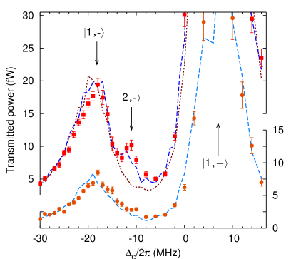
Figure 2: Quantum anharmonicity of the atom-cavity system. Transmitted power as a function of cavity detuning $\Delta_{c}$ for the input powers $0.5$ pW (circles, right scale) and $1.5$ pW (squares, left scale). In this and all following figures, $10$ fW correspond to about $0.01$ intracavity photons, the error bars are s.d. and an offset of $0.5$ fW due to detector dark counts has been removed from the data. The two peaks at $2\pi\times(-18,7)$ MHz represent the two normal modes, which are reproduced by a theory considering only single-photon transitions (dotted line). Note that the maximum of the right peak is beyond the scale of the figure. The quantization of the intracavity light (dashed lines) is required to explain the appearance of the two-photon resonance at $-2\pi\times 11$ MHz at higher intensity.

The quantum anharmonicityBrune et al. (1996) of the energy-level structure reveals itself in the position of the two-photon resonance relative to the normal modes, which is in excellent agreement with equation (1) for a coupling of $g=2\pi\times 11.2$ MHz and a Stark-shifted atom-cavity detuning of $2\pi\times 10.5$ MHz. These values indicate that the coupling is about 70% of the maximally possible value $g_{0}=2\pi\times 16$ MHz at an antinode, and that the trap induces an average Stark shift of $2\pi\times 24.5$ MHz which also corresponds to about 70% of the Stark shift at an antinode of the standing wave dipole trap (the trap depth is 170 nW and the bare atom-cavity detuning is preset to $2\pi\times 35$ MHz). Ideal couplings are not reached due to two reasons: firstly, the atom performs an oscillation in the dipole trap wells; secondly, the position of the trapping wells shifts with respect to the antinodes of the probe light along the cavity axis as the distance from the cavity center increases, therefore atoms which are trapped slightly off the cavity center are not maximally coupled.

We next performed extensive numerical simulations in order to compare the measured spectrum to several cavity QED modelsCarmichael et al. (1994). The simulations closely imitate the experiment, starting from the trapping of single, slow atoms which are injected into the intracavity dipole trap, following up with the measurement protocol which is executed until the atom leaves the trap, and culminating in the same evaluation procedure (see Appendix B). The first set of simulations (only shown for the higher-intensity scan, dotted line in Fig. 2) assumes at most one quantum of energy in the system, thereby allowing us to quantify the contribution due to single-photon transitions. We see that, while the normal-mode resonances are reproduced, there is a large deviation to the measured data precisely at the position of the two-photon resonance. In contrast, another set of simulations (dashed lines) was performed for a quantized cavity mode with three Fock states, $|0\rangle,|1\rangle,|2\rangle$. Apart from the normal modes, these simulations also reproduce the two-photon resonance.

In a second experiment, we explore the quantum regime by scanning the cavity along the vertical arrow in Fig. 1c, using a bare atom-probe detuning of $2\pi\times 21$ MHz and dipole trap power of 140 nW. Fig. 3 displays four scans with different probe laser intensities. The lowest intensity scan (bottom panel) shows a largely flat signal, in agreement with our idea of avoiding the normal modes. Here, the photonic state is close to the vacuum state, with a mean intracavity photon number as low as $0.001$. All higher-intensity scans, however, show a pronounced additional resonance. The deviation between the off-resonance signal, $\Delta_{c}/2\pi\leq-20$ MHz, and the on-resonance signal, $-15$ MHz$\leq\Delta_{c}/2\pi\leq-5$ MHz, gets larger with increasing intensity. Here, we find that a simulation with at most one quantum of excitation (dotted lines) continues to predict a signal with no major modification in the structure, whereas the resonance is globally reproduced with simulations taking into account field quantization. We had to account for four Fock states, indicating that the resonance stems from a two-photon and a weak but rising three-photon transition, the latter transition contributing to broaden the resonance. We also notice an increase in the transmitted intensity at small cavity detunings $|\Delta_{c}|/2\pi\leq 3$ MHz. This is a systematic effect originating from the bare cavity resonance occurring at $\Delta_{c}=0$ with a linewidth of $\kappa=2\pi\times 1.25$ MHz, which could not be completely suppressed in the post-selection process (see Appendix A).

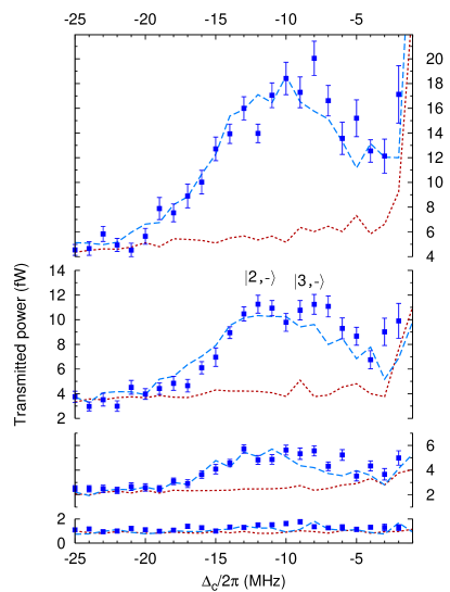
Figure 3: Multi-photon resonances and suppression of single-photon resonances. Transmitted power as a function of cavity detuning $\Delta_{c}$ for input powers of ($0.5,1.5,2.4,3.3)$ pW (from bottom to top, data points). Also shown are the simulations with single-photon (dotted lines) and multi-photon transitions (dashed lines), with the respective positions of the dressed state $|2,-\rangle$ and $|3,-\rangle$.

Under coherent excitation, we expect a mainly quadratic scaling of the transmitted intensity at the frequency of the two-photon resonance and a linear scaling off resonance, i.e. at large cavity detunings $|\Delta_{c}|\gg g$, where all theories coincide. To evaluate the quantum response of the system, the data used for Fig. 3 are averaged over the two-photon region ($-15$ MHz $\leq\Delta_{c}/2\pi\leq-10$ MHz) as well as over the off-resonance region ( $-25$ MHz $\leq\Delta_{c}/2\pi\leq$ $-20$ MHz), for each input intensity. The off-resonant region serves as a reference for the linear single-photon contribution. By taking the difference between the two regions, we isolate the contribution of the two-photon transition, and find a mainly quadratic response of the transmitted intensity versus the input intensity (Fig. 4, circles).

We proceed by comparing the data to a model which assumes the atom to be immobile. This model describes an ideal quantum system, with a well-defined coupling to the mode, as would be desirable for future applications. To this end, we match all the spectra of Fig. 3 to this idealized theory with a common set of parameters $(g,\Delta_{a})$, and find good agreement for $(g,\Delta_{a})=2\pi\times(11.5,1)$ MHz (see Fig. 7). Notice that the coupling $g$ is close to the value obtained for the independent measurements in Fig. 2, whereas the atomic detuning $\Delta_{a}$ is close to zero. The theory spectra are then evaluated in the same way as the measured spectra to obtain the intensity response of the system. The resulting nonlinear curve (solid line in Fig. 4) describes the measured data reasonably well and also shows a mainly quadratic dependency. We hope to further approach the fixed-atom limit in our experiment by extending our cooling protocol from one to three dimensionsNußmann et al. (2005).

For completeness we also analyzed the nonlinear theory of optical bistabilityRempe et al. (1991); Lugiato and Narducci (1992) and found that it is inconsistent with all the measurements presented in this paper, as shown with simulations (Appendix B, Figs. 5 and 6). Specifically, the bistability theory predicts a behavior close to the one we obtained with the theory of coupled oscillators. Explained differently, according to bistability theory, we are operating on the lower branch, where the corresponding nonlinear response is small (dashed line in Fig. 4). Indeed, the reported nonlinearity occurs with an occupation probability of the atomic excited state of at most $0.07$. This is what makes it radically different from and dominant over the standard saturation nonlinearity for a two-state atom.

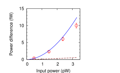
Figure 4: Nonlinear intensity response. Difference between the nonlinear response on the two-photon resonance and the linear single-photon response, together with the prediction from a quantum theory with an immobile atom (solid line). For reference we also show the nonlinearity expected from the saturation of a two-state atom coupled to a classical field (optical bistability theory, dashed line).

In conclusion, our experiment enters a new regime, with nonlinear quantum optics at the level of individual atomic and photonic quanta. In the future we plan to investigate the photon statistics and the spectrum of the light transmitted through the cavity. Once improved cooling forces are implemented to better localize the atom in the cavity mode, new multi-photon states could be produced by applying techniques originally developed for a single atom and single photons to the case of a single atom-cavity system and multiple photons. Other applications in quantum information science include a single-photon transistor, where one photon controls the propagation of another photonChang et al. (2007).

Appendix A Experimental setup and measurement procedure

A.1 Setup

The cavity supports a TEM₀₀ mode near-resonant with the $5{}^{2}S_{1/2}F=3,m_{F}=3\rightarrow 5{}^{2}P_{3/2}F=4,m_{F}=4$ transition of ⁸⁵Rb atoms at wavelength $\lambda=780.2$ nm. The input power is given as the integrated intensity measured in transmission of the resonant empty cavity; the average intracavity photon number is about 0.9/pW (which is approximately $10$ fW for $0.01$ photon as given in the paper). Our cavity does not show birefringence. Consequently, the circular polarization of the input probe light ensures that the atomic transition is closed so that the atom effectively has only two internal states. In addition, a far-detuned dipole-trap laser at 785.3 nm resonantly excites a second TEM₀₀ mode supported by the cavityMaunz et al. (2004), two free spectral ranges detuned from the near-resonant probe mode. Antinodes of probe light and dipole trap coincide in the center of the cavity, such that atoms are localized at regions of strong coupling. The dipole trap laser also serves to stabilize the cavity length. Single atoms are injected into the cavity by means of an atomic fountain and trapped by switching the power of the dipole-trap laser as soon as they reach a region of strong coupling.

A.2 Scanning procedure

After trapping, single atoms are first observed and cooledMaunz et al. (2004) with a weak laser with a power of 0.3 pW and a detuning of $\Delta_{c}$ = 0 for a time interval of $500\ \mathrm{\mu s}$, which we shall call the check interval. This light is then switched to higher power and its detuning is simultaneously adapted in order to probe the system at different frequencies for $100\ \mathrm{\mu s}$ (hereafter the probe interval). The switching between low and high power has been optimized for high speed with minimal overshoots and drifts. This sequence of check and probe intervals is repeated either 20 or 30 times, depending on the expected trapping time of the atom. For Fig. 2, for each data point a different probe frequency $\omega_{L}$ is chosen. For Fig. 3, we vary the cavity length between different trapping events, thereby tuning the cavity frequency $\omega_{c}$. During the probe intervals, the laser is switched to a fixed frequency in the vicinity of $\Delta_{a}$ = 0, the Stark-shifted resonance of the uncoupled trapped atom. We record the photons exiting from the output cavity mirror during the whole measurement and for all atoms and then apply a post-selection protocol as described below.

A.3 Post-selection and accessible scan regions

Atoms which have been strongly heated during probing (due to spontaneous emission or cavity-mediated forcesHechenblaikner et al. (1998)) will follow an enhanced oscillation in the trap, and thus the coupling to the probe mode will be reduced. In this case the interval needs to be removed from the data sample. In order to identify such probe intervals, we check the coupling to the probe mode before and after each probe interval by observing the transmission on the resonance of the empty cavity $\Delta_{c}=0$, which is strongly suppressed in case of a well-localized atom. In a postselection protocol, we select only those probe intervals which show good localization in both enclosing check intervals for further evaluation. About 15% of all intervals in which an atom was present survive this procedure if we require a minimal coupling of $g_{min}=0.6g_{0}$ during both check intervals, where $g_{0}=2\pi\times 16$ MHz is the maximum possible coupling. By comparing the peak positions of the observed normal-mode splitting (Fig. 2) to Eq. 1, we find that the remaining sample shows an average atom-cavity coupling of $g=0.7g_{0}$, exceeding both the cavity field decay rate of $\kappa=2\pi\times 1.25$ MHz and the decay rate of the atomic polarization $\gamma=2\pi\times 3$ MHz.

Such a postselection protocol has already been applied successfully for measurements of the normal-mode spectrumMaunz et al. (2005). Only near $\Delta_{a}\approx\Delta_{c}=0$ in Fig. 3, the post-selection protocol is shot-noise limited since even moderate atom-cavity couplings cause a drop of the transmission to practically zero. Hence we are unable to filter out all of the less-well localized atoms, and the data show a systematic increase of the transmitted intensity for $|\Delta_{c}|\leq 2\pi\times 3$ MHz in Fig. 3. Notice that the simulations, which mimic our experiment, also reproduce this enhancement. Remnants in the transmission signal of the pure cavity resonance have also been reported in a beam of atoms strongly coupled to a cavityChilds et al. (1996), where it was attributed to fluctuations in the number of atoms present in the cavity over time, and for a quantum dot inside a cavityHennessy et al. (2007) where the increase stems from the fluctuations in emitter energy.

Finally, we mention that in Fig. 2 we did not attempt to accurately resolve states $|1,+\rangle$ and $|2,+\rangle$ because this requires extremely long measurement times due to high heating rates in this region, which makes gathering statistics on strongly coupled atoms difficult. To give an order of magnitude, 250 hours of measurement time were required for Fig. 2, and more for Fig. 3. In principle, one could imagine reversing the asymmetry in Fig. 2, such that the peaks for state $|1,+\rangle$ and $|2,+\rangle$ are low while the peaks at $|1,-\rangle$ and $|2,-\rangle$ are enhanced. However, the check interval which is required in our protocol would then coincide with a region of cavity-induced heating, given by ($\Delta_{c}=0,\Delta_{a}<0$), rendering measurements impossible. It is for the same reason that we did not attempt to resolve state $|2,+\rangle$ at $\Delta_{c}>0$ in Fig. 3.

Appendix B Theoretical analysis of the data

B.1 Simulations

B.1.1 General information

We include effects of motion and mismatch between the dipole-trap mode and the near-resonant mode by numerically simulating atomic trajectories in the three-dimensional space from injection into the trap until escape. The measurement procedure is imitated step by step, and we apply the same evaluation protocol to the resulting transmission curves. The motion of the center of mass of the atom is treated classically in all simulations and obeys a Langevin equation with conservative, friction and random forces for diffusion processes. The dipole trap light is modeled by an ac-Stark shift of the atomic levels. We have studied three models. Two types of them are based on the Jaynes-Cummings model for a single atom strongly coupled to a single cavity mode as described by a master equation, including dissipation and expanded by a term accounting for the pumping of the cavity mode. For the first set of simulations we use at most one quantum of excitation (where the spectrum is classical), whereas for the other set we include higher orders to see quantum effects in the spectrum. The third kind of simulation is based on the equations for a two-state atom coupled to a classical field (semiclassical bistability theory).

B.1.2 Simulations using at most one quantum of excitation

Here we truncated the Hilbert space of the atom+mode system after the first doublet of dressed states. This approximation allows for an analytical solution for the forcesHechenblaikner et al. (1998) and hence fast computation; it is appropriate for describing the normal modes in the case of small driving of the systemPuppe et al. (2007b), but inherently excludes any multiphoton effects. We use it in order to quantify the contribution of single-photon transitions to the spectra (dotted lines in Fig. 2 and Fig. 3).

B.1.3 Simulations using more than one quantum of excitation

In a second set of simulations we numerically calculate the excitation of atom and mode as well as the forces on the atom in the presence of higher doublets. In this way, we are able to quantitatively reproduce the measurements (dashed lines in Fig. 2 and Fig. 3) for all spectra. Since there are no analytical expressions available for the quantities of interest, we calculate all numerically, including friction and diffusion tensors which are needed at every step in the integration of the atomic motion. For the simulations shown in Fig. 3, four Fock states were used. Simulations with higher Fock states are beyond our computational resources; as an example, the simulations for Fig. 3 ran for about 150 hours on 30 nodes of a computer cluster. We suspect that the absence of multi-photon transitions of the order four and higher in the code at least partly explains the deviation between theory and experiment in the region of the state $|3,-\rangle$. This is supported by our analysis using the fixed-atom theory, see last section, where we can easily check the convergence of the steady-state solutions such as the average intracavity photon number. Doing so, we indeed see that a fifth Fock state increases the average photon number, and this only around the state $|3,-\rangle$. The convergence around the second dressed state $|2,-\rangle$ has already settled. Further details on the simulations will be shown elsewhere.

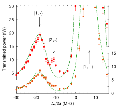
Figure 5: The data from Fig. 2 compared to the simulations using the Maxwell-Bloch equations (semiclassical optical bistability theory). This theory does not reproduce the two-photon resonance and remains close to the fully classical theory. See Discussion for details.

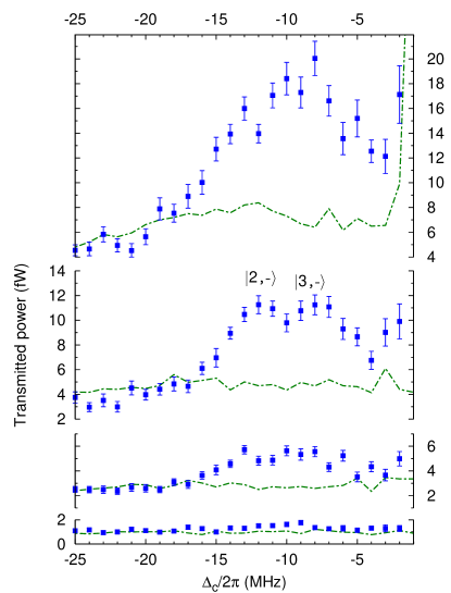
Figure 6: The data from Fig. 3 compared to the simulations using the Maxwell-Bloch equations (semiclassical optical bistability theory). This theory does not reproduce the two-photon resonance and remains close to the fully classical theory. See Discussion for details.

B.1.4 Simulations using the Maxwell-Bloch equations

In a third set of simulations we considered the Maxwell-Bloch equations, which include the possibility of bistability behavior in cavity QED. This theory is important because it allows us to quantify the nonlinearity induced by saturation of the two-state atom due to its coupling to a classical field. The results are shown in the Figs. 5 and 6.

B.2 Analysis of the nonlinear response

In analyzing Fig. 4 we choose to compare the measured nonlinearity to the ideal nonlinearity of the driven Jaynes-Cummings model, where the coupling to the mode is assumed fixed. We start by fitting the whole series of spectra from Fig. 3 to the quantum theory. Here, 15 Fock states are used to ensure convergence of the theory, which sets in at about 5 Fock states. The best match is found for the parameters $(g,\Delta_{a})=2\pi\times(11.5,1)$ MHz, which are fully consistent with our knowledge of the system. Also notice that the value of the coupling differs from that obtained from the analysis from Fig. 2 by only $0.3$ MHz. We use these parameters as input for the semiclassical and classical theories. The data and theories are shown in Fig. 7.

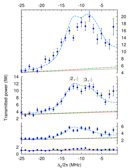
Figure 7: The data from Fig. 3 compared to the theories for an atom with fixed coupling and detuning, in the classical (dotted lines), semiclassical (dash-dotted lines) or quantum (dashed lines) cases. For fit parameters, see Discussion.

To achieve an overall agreement of quantum theory to the data, we need to shift the theory curves upwards by a small constant offset $(0.8,1.5,2,2.5)$ fW for the consecutive spectra. For consistency, the same offset has been applied to all theories. We note two things about this offset: first, it originates from atomic motion because it is only needed within the frame of a fixed-atom theory, while the quantum simulations, which include the motion, directly match the measurements. Second, this offset is frequency-independent. Therefore, it is present in the far off-resonant region, $|\Delta_{c}|\gg g$, where all theories asymptotically coincide. Indeed, one can see that the off-resonant region is already correctly described by the single-photon simulations. Also notice that the fixed-atom theory needs to be shifted upwards already for the lowest intensity scan at $0.5$ pW, where the influence of two-photon transitions on the spectrum is small. This means that the offset is largely single-photon induced. We therefore conclude that the offset stems from the motion of the atom in the trap which leads to a small background transmission caused by single-photon transitions. Besides this caveat, the quantum fixed-atom theory reproduces the observed peak structures for all four input intensities using one common pair of parameters $(g,\Delta_{a})$. Only in the case of the highest input intensity ($3.3$ pW), the observed peak height does not quite reach the theory curve. It is plausible to assume that this region is affected most by heating, since here the light intensity and atomic excitation reach a maximum, although remaining at a low absolute value (the excitation probability is below $0.05$ as deduced from a fixed-atom theory and $0.07$ as deduced from the simulations).

To determine the nonlinearity of the intensity response from the fixed-atom theory, we proceed in the same way as for the experiment: for each intensity, we average on the two-photon resonance signal and off-resonance signal and calculate the difference to obtain the multi-photon contribution (solid line in Fig. 4). The resulting intensity response shows a mainly quadratic behavior for the given intensities. We do the same for the nonlinear response expected from the Maxwell-Bloch equations (dash-dotted line in Fig. 7, dashed line in Fig. 4).

Finally, in Fig. 7 notice the double-peak structure of the resonance, which stems from a two-photon and a weak three-photon transition. For our parameters, the higher multi-photon transitions do not appear as separate peaks on the right of state $|3,-\rangle$, but do raise the transmission around this peak.