An absorption origin for the X-ray spectral variability of MCG–6-30-15

Abstract

Context. The Seyfert I galaxy MCG$-6$-30-15 shows one of the best examples of a broad “red wing” of emission in its X-ray spectrum at energies $2<E<6.4$ keV, commonly interpreted as being caused by relativistically-blurred reflection close to the event horizon of the black hole.

Aims. We aim to test an alternative model in which absorption creates the observed spectral shape, explains the puzzling lack of variability of the red wing and reduces the high reflection albedo, substantially greater than unity, that is otherwise inferred at energies $E>20$ keV.

Methods. We compiled all the available long-exposure, high-quality data for MCG$-6$-30-15: 522 ks of Chandra hetgs, 282 ks of XMM-Newton pn/rgs and 253 ks of Suzaku xis/pin data. This is the first analysis of this full dataset. We investigated the spectral variability on timescales $>20$ ks using principal components analysis and fitted spectral models to “flux state” and mean spectra over the energy range $0.5-45$ keV (depending on detector). The absorber model was based on the zones previously identified in the high-resolution grating data. Joint fits were carried out to any data that were simultaneous.

Results. Multiple absorbing zones covering a wide range of ionisation are required by the grating data, including a highly ionised outflowing zone. A variable partial-covering zone plus absorbed low-ionisation reflection, distant from the source, provides a complete description of the variable X-ray spectrum. A single model fits all the data. We conclude that these zones are responsible for the red wing, its apparent lack of variability, the absorption structure around the Fe K$\alpha$ line, the soft-band “excess” and the high flux seen in the hard X-ray band. A relativistically-blurred Fe line is not required in this model. We suggest the partial covering zone is a clumpy wind from the accretion disk.

1 Introduction

The galaxy MCG$-6$-30-15 is a well-known Seyfert type I at redshift $z=0.00775$, and was one of the first to show evidence in ASCA observations for a broad wing of emission extending to lower energies from the 6.4 keV Fe K$\alpha$ line (Tanaka et al., 1995). A common interpretation of this emission is that it arises as reflection from the inner regions of the accretion disc, where the photon energy is smeared to low energies by relativistic effects (e.g. Tanaka et al., 1995; Iwasawa et al., 1996). The existence of the “red wing” has been subsequently confirmed by more recent observations with XMM-Newton and Suzaku (Wilms et al. 2001, Fabian et al. 2002, Vaughan & Fabian 2004, Reynolds et al. 2004, Miniutti et al. 2007), but investigation of models for the physical origin of this component have concentrated on the “blurred reflection” hypothesis (see Brenneman & Reynolds 2006 for a summary of the history of analysis of the X-ray spectrum).

However, it has long been known that absorption can conspire to produce continuum shapes similar to those observed in the AGN with red wings (e.g. in NGC 3516, Turner et al. 2005 and NGC 3783, Reeves et al. 2004), and MCG$-6$-30-15 itself is known to show strong absorption lines indicating the presence of absorption by zones of gas with a very broad range of ionisation. In the Fe K$\alpha$ region both Young et al. (2005) in high-resolution Chandra heg data and Miniutti et al. (2007) in Suzaku xis data detected lines at 6.7 and 7.0 keV, most likely identified as Fe xxv and Fe xxvi with an outflow velocity $\sim 1800$ km s^-1. This identification of a highly ionised outflowing zone is substantiated by the detection of matching lines from Si xiv and S xvi at 2.0 and 2.6 keV in the Chandra meg data (Young et al., 2005). High-resolution data at softer energies also reveal lines from a broad range of ionisation: Lee et al. (2001) showed that at least two zones of gas with ionisation parameter $\log\xi\simeq 0.7$ and 2.5 were required to explain the lines detected in the Chandra meg data, and these lines were further confirmed by detections in XMM-Newton rgs data (Turner et al., 2003, 2004). Lee et al. (2001) also interpreted the strong edge observed at 0.7 keV as being an edge from Fe i, possibly arising in dust grains. To date there has been little published evaluation of the possible effect of such zones on the observed continuum from this source, although some analyses have included some of the known absorption zones (e.g. Brenneman & Reynolds, 2006): in this paper we shall investigate absorption-dominated models that both explain the continuum shapes and the absorption lines that are observed.

A further motivation for this work is that it has been recognised for some time that the red wing component is surprisingly constant in amplitude (Iwasawa et al., 1996; Vaughan & Fabian, 2004) (although Ponti et al. 2004 did find evidence for additional variability around 5 keV in the 2000 XMM-Newton observation). If the red wing emission is indeed reflected emission from the accretion disk we would expect its amplitude to vary in phase with the primary continuum, counter to what is found in most observations: the only occasion on which it has been inferred that this expected property did occur was when the source was in its lowest flux state, as observed with XMM-Newton in 2000 (Reynolds et al., 2004). The general lack of red wing variability has led to the development of a “light-bending” model in which the observed primary continuum variations are caused by variations in height of the illuminating continuum coupled with distortions of photon geodesics near the black hole, rather than by rest-frame intensity variations, so that the reflected emission appears more constant than the primary continuum seen by the observer (Fabian & Vaughan, 2003; Miniutti et al., 2003; Miniutti & Fabian, 2004). The same model has also been invoked to explain the high flux observed at $E>20$ keV in Suzaku pin data as being the Compton reflection “hump” enhanced in amplitude by the same light-bending effects (Miniutti et al., 2007). Other models that seek to explain the constant red wing amplitude (e.g. Merloni et al., 2006; Nayakshin & Kazanas, 2002; Życki, 2004) do not explicitly produce an explanation for the high energy excess, and some are unlikely to apply to MCG$-6$-30-15 (Życki & Różańska, 2001) and on long timescales (Miller et al., 2007, hereafter M07). However, light-bending is not the only way to produce a constant red wing and a high energy excess. The constancy of the component could be explained if the reflection were distant from the primary source, so that light travel time smooths out any illumination variations, or models with a variable covering fraction of absorption can produce a similar effect (see the discussion in M07 and Turner et al. 2007, hereafter T07). Furthermore, the high energy excess may be explained as either being a combination of reflection with no light-bending enhancement and a contribution from a highly absorbed (N${}_{\rm H}\ga 10^{23}$ cm^-2) continuum component: or indeed perhaps even an absorbed component alone. The existence of a high-energy excess on its own does not require light-bending or relativistic blurring of reflected emission.

Thus our aim in this paper is to investigate the extent to which the full X-ray spectrum of MCG$-6$-30-15 may be explained by the effect of absorption of the intrinsic emission. We are aided in this by two key advances since previous analyses. First, there now exists a significant body of high quality data, from three independent observatories, Chandra , XMM-Newton and Suzaku . The Suzaku data include low-resolution spectral measurements up to $\sim 45$ keV, and in this paper we analyse, for the first time, the entire set of CCD-resolution data that is available for this source, and we test physical models against the full energy range available, $\sim 0.5-45$ keV. We also test the models for consistency with the high-resolution Chandra hetgs and XMM-Newton rgs data.

The second advance is to make as much use as possible of the spectral variability exhibited by this (and other) AGN: the spectrum appears to change shape in a systematic way as the total X-ray flux of the source varies, implying that the emission we see is made up of a number of components whose individual spectra differ. We use a method of principal components analysis, described below, that retains the full spectral information content of the data, to first set the basic parameters of models describing each of those components, and then we test the resulting model against the actual data.

2 Analysis methods

2.1 Principal components analysis

The starting point for the physical models developed in this paper is a model-free principal components analysis (hereafter PCA) of the spectral variations of MCG$-6$-30-15. Such an analysis was first applied to this source with low spectral resolution by Vaughan & Fabian (2004). In this paper we use the method developed and described by M07, which uses singular value decomposition to achieve a principal components decomposition of the spectral variations whilst retaining the full spectral resolution of XMM-Newton pn and Suzaku xis data. In the case of the analysis of Mrk 766 (M07) this provided significant additional information, as it revealed the presence of absorption edge and line features associated with a hard spectral component, and it provided model-independent evidence for the presence of both ionised absorption associated with the principal varying component and also ionised Fe emission. We shall see below that similar features appear in MCG$-6$-30-15.

The optimal-resolution PCA procedure adopted is identical to that of M07 and we refer to that paper for full details of the method. The random errors in the principal components arising from photon shot noise are estimated by a Monte Carlo simulation, in which the PCA is repeated for synthetic spectra that are perturbed by random noise about the true spectra. The resulting errors are correlated between the principal components but do allow some estimation of the effect of shot noise.

The basic output from the PCA is a set of eigenvectors, each one representing the spectrum of an additive mode of variation. The generic varying power-law, that is a ubiquitous feature of AGN X-ray spectra, appears as “eigenvector one” in this analysis. In addition it was found in Mrk 766 that the bulk of the variation could be described by a single eigenvector superimposed on a quasi-constant component of emission, which in that paper was named the “offset component”. But there is not a unique association of physical components with the eigenvectors and offset components. For example, there could in the source be components with exactly the spectra of eigenvector one (a varying absorbed power-law) and the offset component (which could be reflected emission from an extended region where light-travel-time effects dampen any intrinsic variation in the illumination). Alternatively there could instead be two variable additive components whose variations are correlated, such that eigenvector one represents the net overall effect of their joint variation. A possible physical model that achieves the latter is if spectral variations are caused by variations in the covering fraction of an absorber passing across an extended source - in this case the offset component represents the view of the source when it is most covered, the highest flux state represents the source when it is most uncovered, and eigenvector one represents the difference between these states. These interpretations can produce identical PCA results and are indistinguishable: we must rely on physical models to attempt to discern which interpretation is closest to reality. In practice, it may be that both a quasi-constant reflection component and a variable covering-fraction absorber are present, a hybrid model also mentioned by M07 and T07.

Such an analysis effectively assumes that the spectral variations may be described by additive spectral components. In the case of Mrk 766 it was found that although the chief variations could be modelled in this way, there were still significant non-additive variations which were found to be caused by absorption variations (M07, T07). In this parallel analysis of MCG$-6$-30-15 we shall first investigate the PCA, and fit models to the principal components, and then also explore directly fitting to the data the models that arise from the PCA. We shall not, however, explore temporal absorption variations, although we shall see that there is evidence for these also in MCG$-6$-30-15.

2.2 Data grouping and spectral fitting

The principal statistical tool used here will be goodness-of-fit testing using the binned $\chi^{2}$ statistic. As in M07, we adopt an optimum spectral binning of the data, with spectral bins whose width in energy are equal to half the energy-dependent instrumental FWHM. Any spectral features arising in finer binning cannot be intrinsic to the source and we should not fit models with binning finer than this. It is commonplace in the literature on X-ray observations for goodness-of-fit statistics to be quoted with much finer binning than the instrumental resolution: such reported values can be misleading, in that the reduced $\chi^{2}$ in such cases may appear low, but the goodness-of-fit probability might in fact be rather poor. The sensitivity to departures of the model from the data is significantly reduced with binning that is too fine. To illustrate this here with a simplified example, suppose data is divided into $n$ bins, fit by a model with $p$ free parameters that yields a goodness-of-fit $\chi^{2}_{n}=n-p+\Delta\chi^{2}$, where $\Delta\chi^{2}$ is the excess $\chi^{2}$ over the expectation value $n-p$ for a well-fitting model. If the data are then more finely divided into $m$ bins, $m>n$, with the data errors increasing as the inverse square root of the bin width, then if the model does not have any variations on this finer scale we can use the properties of the non-central $\chi^{2}$ distribution to infer an expected new goodness-of-fit, $\chi^{2}_{m}\simeq m-p+\Delta\chi^{2}$ where $\Delta\chi^{2}$ has the same value as in the case of $n$ bins. For example, for $\chi^{2}_{n}=400$, $n=300$, we would obtain $\chi^{2}_{m}=3100$ for $m=3000$ (adopting the simplification $p=0$). The first case has a reduced $\chi^{2}=1.33$ and the model would be rejected at significance level $p=10^{-4}$. The second case has reduced $\chi^{2}=1.033$ and the model would only be rejected at $p=0.1$.

In this paper we adopt the optimum energy binning for maximum sensitivity, and hence the goodness-of-fit statistics will indicate worse fits than if we had adopted finer energy binning. Where relevant, we shall compare goodness-of-fit with previous published results for MCG$-6$-30-15 by calculating $\chi^{2}$ with similar binning to that adopted by other authors.

2.3 Systematic uncertainties in data and models

Photon counts are everywhere sufficiently high for the approximation that the error in each bin has a normal distribution to be valid. However, the datasets being analysed comprise long observations on this bright AGN, and in fact the goodness-of-fit is no longer dominated entirely by photon statistics, especially at the low energy end of the spectra.

Systematic errors in the data exist through uncertainty in the calibration. These uncertainties have not yet been fully quantified for Suzaku , but for XMM-Newton it seems that there can be energy-dependent discrepancies of 5-10 percent between pn and mos instruments, depending on the spectrum of the source, and discrepancies of up to 20 percent in the XMM-Newton pn v. Suzaku xis cross-calibration (Stuhlinger, 2007).

There are also systematic uncertainties in the models, in the sense that, in order to keep the number of free parameters to a minimum, we inevitably fit simplified models to what in reality must be a complex set of emission and absorption processes. For example, it is commonplace to use the reflion models of Ross & Fabian (2005) to model reflection spectra. However, those models assume a constant density slab at normal inclination, whereas in practice there must be a complex geometry. Emission-line fluxes in particular will be orientation dependent (e.g. George & Fabian, 1991; Życki & Czerny, 1994), and it has been suggested that a disk atmosphere in hydrostatic pressure equilibrium would result in a quite different spectrum (Done & Nayakshin, 2007). Such systematic “model error” is difficult to quantify.

There is no rigorous way of taking such systematic errors into account in the goodness-of-fit testing. Within xspec (Arnaud, 1996) it is possible to treat the systematic error as being a constant fractional error that is added in quadrature with the random error. In this paper we adopt as standard a fractional systematic error of 3 percent, a value that is around the lowest systematic uncertainty we might expect given the cross-instrument comparisons that have been made to date. Where relevant, when comparing our results with previous results in the literature, we shall quote goodness-of-fit statistics assuming zero systematic error.

3 The data

3.1 XMM-Newton data

The XMM-Newton dataset comprises two observations made in 2000, previously described and analysed by Wilms et al. (2001), Reynolds et al. (2004) and Ponti et al. (2004), and three closely-spaced observations made in 2001, previously described and analysed by Fabian et al. (2002), Vaughan & Fabian (2004) and Brenneman & Reynolds (2006). The observation dates, IDs, duration of the observations and on-source exposure times after screening are given in Table 1.

Table 1: Datasets used in this analysis, giving observation date, ID, observation duration and on-source exposure time (pn times are given for XMM-Newton , xis times are given for Suzaku ).

Observatory	date	ID	dur	exp
			/ks	/ks
XMM-Newton	11 Jul 2000	0111570101	43.2	41.1
XMM-Newton	11-12 Jul 2000	0111570201	46.0	32.3
XMM-Newton	31 Jul 2001	0029740101	79.5	57.7
	- 1 Aug 2001
XMM-Newton	2-3 Aug 2001	0029740701	125.9	69.0
XMM-Newton	4-5 Aug 2001	0029740801	125.0	81.5
Suzaku	9-14 Jan 2006	700007010	354.2	103.5
Suzaku	23-26 Jan 2006	700007020	215.3	72.1
Suzaku	27-30 Jan 2006	700007030	208.3	77.4
Chandra	19-27 May 2004	4759-4762	530.0	521.8

In this analysis we use data from the epic pn CCD detector (Strüder et al., 2001) in the energy range $0.4-9.8$ keV. Data from the Metal Oxide Semi-Conductor (mos) CCDs were not used as they suffer significant photon pileup and inferior signal-to-noise. All pn observations utilised the medium filter and the small window mode. Data were processed using sas v7.0 using standard criteria with instrument patterns 0–4 and removing periods of high background (where the rate in the background cell exceeded 0.15 count s^-1). Source data were extracted from a circular cell of radius $50^{\prime\prime}$ centred on the source, and background data were taken from a source-free region of approximately the same size within the same pn chip. The total 2000 and 2001 pn exposures were 73 ks and 208 ks, respectively. The typical deadtime correction was a factor 0.7. During 2000 the mean pn count rate was $\sim 3.709$ $\pm 0.010$ count s^-1 and during 2001 $\sim 4.908$ $\pm 0.005$ count s^-1 in the 2–10 keV band. The mean background level in the screened data was $<1$% of the mean source rate in this band.

We also used higher resolution spectra from the Reflection Grating Spectrometer (rgs, den Herder et al. 2001) which were taken from the pipeline processing and were coadded for each rgs grating to yield two spectra for each of the 2000, 2001 epochs. As the individual exposures were taken just days apart and the source was centred the same on the detector for each observation, the responses were indistinguishable for the parts that were coadded and this summation did not result in any significant loss of effective resolution within the data. The total rgs 1 exposure was 108 ks for 2000 and 331 ks for 2001; the rgs 2 exposure was 105 ks for 2000, 323 ks for 2001. During 2000 first-order rgs data yielded 0.71$\pm 0.003$ count s^-1 and $0.64\pm 0.03$ count s^-1 for the summed rgs 1 and rgs 2 data respectively, and during 2001, 0.89$\pm 0.002$ count s^-1 and 0.90$\pm 0.02$ count s^-1 for rgs 1 and rgs 2, respectively. The rgs background level was $\sim 11\%$ of the total count rate.

3.2 Suzaku data

The Suzaku dataset comprises three observations made in 2006 as tabulated and previously described and analysed by Miniutti et al. (2007). Because of the much shorter duration and the changing instrumental response we do not use a shorter observation made on 2005 Aug 17. The observation dates, IDs, total duration of the xis observations and on-source exposure times after screening are given in Table 1 (xis 0 typically had a slightly lower on-source exposure time than the other detectors). We used xis and hxd pin events from v2.0.6.13 of the Suzaku pipeline. Both the xis and hxd pin data were reduced using v6.3.2 of HEAsoft and screened with xselect to exclude data during and within 436 seconds of entry/exit from the South Atlantic Anomaly (SAA). Additionally we excluded data with an Earth elevation angle less than 5^∘ and Earth day-time elevation angles less than 20^∘. A cut-off rigidity (COR) of $>6$ GeV was applied to lower particle background. The source was observed at the nominal centre position for the xis for all observations. The xis-fi CCDs were in $3\times 3$ and $5\times 5$ editmodes. Data from the back-illuminated xis 1 detector were not used because its effective area is lower than that of the front-illuminated XIS 0/2/3 at 6 keV, while its background rate is larger at high energies. For the xis CCDs we selected good events with grades 0,2,3,4, and 6 and removed hot and flickering pixels using the sisclean script.

The xis products were extracted from circular regions of 2.9′radius while background spectra were extracted from a region of the same size offset from the source (and avoiding the chip corners with the calibration sources). The response matrix (rmfs) and ancillary response (arf) files were then created using the tasks xisrmfgen and xissimarfgen, respectively. xissimarfgen accounts for the hydrocarbon contamination on the optical blocking filter. The background was $<1\%$ of the total xis count rate in the full xis band for each CCD. The xis 0,2,3 were combined to produce a single xis-fi spectrum, along with the response files with the appropriate (1/3) weighting.

The pin background events file was provided by the hxd instrument team, used in conjunction with the source events file to create a common good time interval set applicable to both the source and background. The background events file was generated using ten times the actual background count rate, so we increased the effective exposure time of the background spectra by a factor of 10. We found the deadtime correction factor using the hxddtcor task with the extracted source spectra and the unfiltered source events files. The total on-source exposure time, after screening, was 292 ks, somewhat longer than for the xis. The contribution of the cosmic X-ray background (Boldt, 1987; Gruber et al., 1999) was taken into account as described later. The source comprised 26% of the total counts, clearly above the $1\sigma$ 3.2% hxd pin background systematic level. The response file ae_hxd_pinxinome1_20070914.rsp provided by the instrument team was used in all the spectral fits. In the subsequent analysis, the pin flux has been decreased by a factor 1.09 to be consistent for observations at the xis pointing position with the cross-calibration study of Koyama et al. (2007), revised for the Suzaku revision 2 analysis pipeline.

3.3 Chandra hetgs data

Chandra hetgs exposures for MCG$-6$-30-15 were taken during May 2004 yielding 522 ks of good data (OBSIDs 4759-62) as detailed by Young et al. (2005) (Table 1 gives the summed duration of each of the four OBSIDs). An earlier observation made in 2000 has been analysed by Lee et al. (2001) but is not included here owing to its much shorter duration. Data were reduced using ciao v3.4 and caldb v3.4.0 and following standard procedures for extraction of HETG spectra, except that we used a narrower extraction strip than the tgextract default. This reason for the default processing cut-off is that the overlap of the MEG and HEG strips depends on the extraction strip widths, and if the latter are too large, a larger intersection of the MEG and HEG strips results, cutting off the HEG data prematurely. Specifically, we used width_factor_hetg=20 in the tool tg_create_mask, instead of the default value of 35. As the hetgs spectra have a very low signal-to-noise ratio it was necessary to coadd the positive and negative first-order spectra, and coadd all four OBSIDs, to create a high quality summed first-order heg and meg spectra for fitting. After such co-addition, we binned the spectra to 4096 channels before grouping. The summed Chandra hetgs exposure yielded a 2–7 keV count rate $\sim 0.1559\pm 0.0006$ count s^-1 and $\sim 0.1926\pm 0.0007$ count s^-1 in the summed heg and meg first order spectra, respectively. The background level in this case is so low as to be negligible.

4 Results - the Principal Components

4.1 Principal components analysis

We first analyse the XMM-Newton and Suzaku data using PCA, following the methods described above and in M07. There are a number of statistical measures we can employ to test how good the PCA model fits the data, and how many components are required. Tables 2 and 3 show for the two datasets how much of the observed variance is accounted for by each component, and how well the data are described by a source model comprising the offset component plus the first $n$ eigenvectors, measured by the $\chi^{2}$ statistic. The latter is the mean $\chi^{2}$ averaged over all timeslices. It can be seen that at energies above 2 keV a single eigenvector is all that is required in addition to the offset component to adequately describe the spectral variations. Considering the whole energy range, more eigenvectors are needed, indicating the effects of variable absorption as found for Mrk 766 (M07, T07). In fact, there are some time slices that have anomalously high $\chi^{2}$ values, as indicated in Fig. 1 which shows for each timeslice in the Suzaku dataset the value of $\chi^{2}$ obtained for the full energy range when allowing an increasing number of components. Most time slices are well fit by a single varying component, but there are a few time slices, especially in the first observation, where even adopting 3 principal components still leads to a high $\chi^{2}$ value. Some of these “badly fitting” events are correlated in time with each other, and we suspect that they are caused by absorption variations, as found for Mrk 766 (T07).

Table 2: Statistics of the Principal Components Analysis of the Suzaku data. Component 0 indicates the fit of the mean spectrum alone, subsequent components are eigenvectors ordered by their eigenvalues (column 2). Column 3 shows the fractional variance accounted for by each component, columns 4 and 5 give the goodness-of-fit ($\chi^{2}$ and number of degrees of freedom) for the entire range and for $2-50$ keV alone.

comp.	eigenvalue	fractional	$\chi^{2}$	/dof	$\chi^{2}$	/dof
		variance	0.4–50 keV		2–50 keV
0	-	-	4736	171	1661	114
1	0.00167	0.645	235	170	113	113
2	0.00052	0.201	216	169	108	112
3	0.00012	0.046	205	168	104	111
4	0.00005	0.019	191	167	99	110
5	0.00002	0.009	165	166	93	109

Table 3: Statistics of the Principal Components Analysis of the XMM-Newton data, with columns as for Table 2 with appropriate energy ranges.

comp.	eigenvalue	fractional	$\chi^{2}$	/dof	$\chi^{2}$	/dof
		variance	0.4–9.8 keV		2–9.8 keV
0	-	-	22322	167	3922	125
1	0.000977	0.928	953	166	123	124
2	0.000016	0.015	325	165	105	123
3	0.000012	0.012	208	164	86	122
4	0.000009	0.008	161	163	75	121

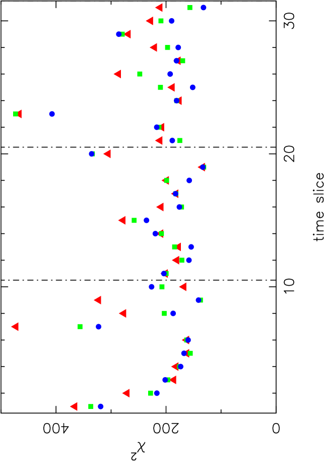
Figure 1: $\chi^{2}$ values for the full energy range for each time slice in the Suzaku data, assuming a constant component plus: a single eigenvector (red triangles); two eigenvectors (green squares); or three eigenvectors (blue circles). The number of degrees of freedom is 170-168 respectively. Dashed vertical lines indicate the start of a new observation, separated in time from the previous observation.

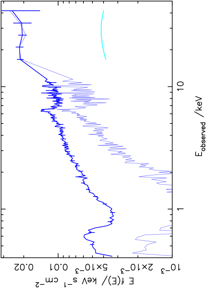
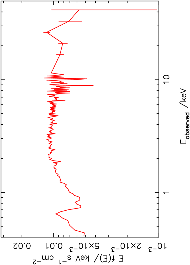
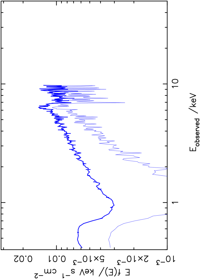
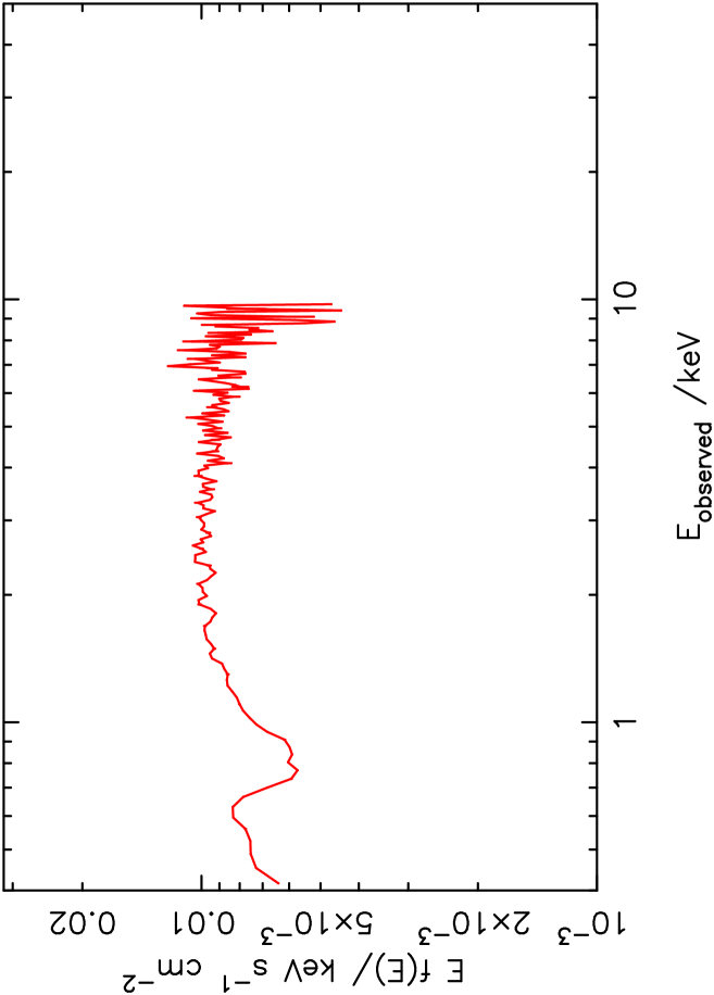
Figure 2: Principal component spectra for (top) Suzaku data and (bottom) XMM-Newton data. Left-hand panels show limits on the offset component, right-hand panels show eigenvector one, top curve (red), and eigenvector two, lower curve, falling below the plot boundary (green). Spectral points in the range $0.4-11$ keV are from the pn or xis instruments, those in the range $15-45$ keV are from the pin. See text for further details.

The resulting component spectra are shown in Fig. 2. The offset component is not uniquely defined, but exists between the limits shown: only a systematic shift between those limits is allowed (more specifically, the offset component can be shifted by linear combinations of whichever eigenvectors are allowed to describe the variations). As well as the pin detector background, a contribution from the expected cosmic X-ray background has also been subtracted from the pin data, using the same model and amplitude as Miniutti et al. (2007). This component is also plotted, so it may be seen that this makes an important but not dominant contribution to the total measured pin flux.

Random uncertainties on the offset component and eigenvector one are estimated from a Monte-Carlo realisation as described in section 2.1 and are shown on the upper curve only. Only every fifth error bar is plotted, for clarity. Eigenvector one is plotted with an amplitude equal to the mean value in each dataset.

For clarity we do not plot further eigenvectors: although the presence of eigenvector two seems statistically significant, its amplitude is low and it has little effect on the spectral shape of the offset and first eigenvector components.

4.2 Spectral models

4.2.1 Overview

As in Mrk 766, the offset component has a hard continuum shape with a soft excess, a weak line at the energy of low ionisation Fe K$\alpha$, an edge and absorption lines, also detected by Miniutti et al. (2007) in the total spectrum. The pin data reveal a high flux in the $15-40$ keV range as found by Miniutti et al. (2007), although we note that with improved deadtime correction and background subtraction there is now no indication of any fall-off to higher energies, consistent with the general lack of cut-offs in AGN spectra at these energies (e.g. Panessa et al., 2008). The first eigenvector has the appearance of an absorbed powerlaw. The most basic interpretation of these two components are that the offset component is a reflection component and eigenvector one is a variable-amplitude absorbed powerlaw, the variations of which yield the observed spectral variability. This model has formed the basis for previous analyses of the X-ray spectrum of MCG–6-30-15 and other AGN (e.g. Fabian et al. 2002; Fabian & Vaughan 2003; Vaughan & Fabian 2004) and is the one we adopt here. An alternative would be to consider the possible spectral variations arising from a thermal comptonising plasma (e.g. Haardt et al., 1997), but such models appear to be disfavoured for the analysis presented here: first, the soft excess is not bright enough compared with the Haardt et al. (1997) model; second, in that model it is expected that the Compton excess should decrease as the $2-10$ keV flux increases, counter to what is observed; and finally the PCA presented here provides strong evidence that the source variability is primarily well described by the additive variations of a small number of components.

We shall start by fitting basic models to these components. All fits were made with xspec v11 (Arnaud, 1996). Models of ionised absorption were created using xstar (Kallman et al., 2004) which models the absorption from a spherically-symmetric shell of gas around a central source. It is particularly important to include the best possible atomic physics calculations in the absorber models: Kallman et al. (2004) have shown how improved calculations lead to bound-free edges that are significantly less sharp than would otherwise be obtained, and those authors point out that this may have a significant effect on the interpretation of the edge around Fe K$\alpha$. In the models made here, fittable parameters were the absorbing column, the ionisation parameter $\xi$ at the inner face of the absorbing shell and the redshift. For simplicity, solar abundances were assumed for all models. The ionising spectrum was assumed to be a power-law of photon index $\Gamma=2.2$ between 13.6 eV and 13.6 keV: other values of photon index can produce similar absorption spectra but with a shift in the effective ionisation parameter. The gas density was assumed to be $10^{10}$ cm^-3 for all zones except the highest ionisation zone, where a value $10^{8}$ cm^-3 was assumed. Although this parameter affects the absorption spectral shape, this again is largely degenerate with the ionisation parameter, although if the assumed absorbing shell is sufficiently thick (as may occur for the combination of high $\xi$ and low density values) then there can be significant variation in $\xi$ through the zone arising from inverse-square-law dilution, thus leading to a broader range of ionisation states than might be the case in a denser, thinner shell of gas. All the absorption models are affected by such uncertainties. We adopt units of erg cm s^-1 for $\xi$.

4.2.2 Joint fit to eigenvector one and offset components

Qualitatively, the PCA “eigenvector one” in both the Suzaku and the XMM-Newton data has the appearance of a powerlaw affected by ionised absorption. In reality the absorbing zones are complex, and their physical parameters are unlikely to be unambiguously measurable in data with CCD resolution. However, we know a priori of the existence of ionised absorbing zones from the previous analyses of Chandra and XMM-Newton high-resolution grating data, so we can start by seeing whether a model that includes those zones can explain the CCD spectra we observe.

We first create a model based on the simplest interpretation of the PCA, namely that the eigenvector one represents a variable-amplitude powerlaw, with ionised absorption, and that the offset component arises from distant reflection, with light travel-time erasing any reflected amplitude variations. The primary absorbing layers that have already been identified in the grating data comprise:

• Zone 1 with $\log\xi\simeq 2$ (Lee et al., 2001)

• Zone 2 with $\log\xi\simeq 0.5$ (Lee et al., 2001)

• Zone 3, a highly ionised, $\log\xi\ga 3.5$, outflow at line-of-sight velocity $v\simeq 1800$ km s^-1 (Young et al., 2005). The $6.7$ and $6.97$ keV lines only appear in the offset component in the PCA, not on eigenvector one, so for now we assume that this zone is only associated with the offset component (when fitting to the data later, we allow zone 3 to absorb all components). This zone also produces velocity-shifted lines of 2.0 keV Si xiv Ly$\alpha$ and 2.62 keV S xvi Ly$\alpha$ which were observed by Young et al. (2005) in the Chandra meg data. In this absorption layer the ratio of the 6.7 and 6.97 keV lines depends on both the ionisation and on the microturbulent velocity dispersion of the gas, since the lines are easily saturated, and the relatively high equivalent width of the lines is most easily achieved by models with line broadening. Hence the absorption model is broadened by a velocity dispersion of 500 km s^-1, consistent with the findings of Young et al. (2005) (see section 5), and we fix the ionisation parameter at $\log\xi=3.85$ as described later in section 5.1.

• Fe I edge at 0.707 keV. A further feature apparent in the high-resolution data, but not in data of CCD resolution, is the complex absorption edge structure at $\sim 0.7$ keV, discussed extensively by Branduardi-Raymont et al. (2001), Sako et al. (2003), Lee et al. (2001) and Turner et al. (2003, 2004). Here we adopt the model advocated by the last three authors, in which the edge primarily arises from neutral Fe which is possibly in the form of dust grains (see Ballantyne et al. 2003b for a discussion of the possible location and origin of the dust). Rather than attempting a complex model of this region, we simply add a single edge at the systemic redshift whose rest-frame energy corresponds to the 0.707 keV l3 Fe I edge (Lee et al., 2001), with fixed edge optical depth $\tau=0.4$, as indicated by the high-resolution data (in fitting to the grating data later, we allow $\tau$ to be a free parameter).

We initially model the offset component as low-ionisation reflection, adopting the constant density slab model of Ross et al. (1999) and Ross & Fabian (2005) and calculated by the xspec extended reflionx model made available by those authors. The illumination was assumed to be the same powerlaw for both eigenvector one and the offset component, and absorbing zones 1 & 2 and the dust edge were assumed to cover both components. We assume the 6.4 keV Fe K$\alpha$ emission line arises in the low-ionisation reflection, which in the reflionx models restricts the ionisation to be $\xi\la 120$ erg cm s^-1 for photon index $\Gamma\simeq 2.2$. Better overall $\chi^{2}$ values may be obtained by relaxing this constraint, but such fits are inconsistent with the data in the Fe K$\alpha$ regime, so we apply this constraint throughout. It is possible, of course, that the 6.4 keV line arises in photoionised gas, and not from reflection, and it is also possible that there is a wide range of reflection ionisation (e.g. Ballantyne et al. 2003a), but we shall start with simpler models to evaluate the extent to which they describe the observations.

Further constraints on the model are available from the soft band high resolution XMM-Newton rgs and Chandra hetgs grating data. One particular feature is that there is no evidence in any of the grating data for strong 0.65 keV O viii emission, whereas the reflionx models lead us to expect significant line emission in the soft band to match the observed 6.4 keV Fe K$\alpha$ emission, if this arises from reflection. So it must be that either the Fe K$\alpha$ line does not have a reflection origin, or its ionisation is sufficiently low that no O viii emission is expected, or the reflection is affected by absorption in the soft band. In the models described here, we adopt the latter solution, although we should bear in mind the former possibilities. This interpretation of the Fe line leads to the need to allow a further layer of absorption associated with the distant reflection, zone 4, which may in fact be an atmosphere associated with the reflection region. This absorption zone hardens the reflection spectrum and thus for a given $2-10$ keV flux increases the flux in the Suzaku pin band, and allowing the reflection to be ionised explains why the equivalent width of the Fe emission is lower than expected from neutral reflection (George & Fabian, 1991; Życki & Czerny, 1994; Ross et al., 1999). We should expect some emission from the absorbing gas in zone 4, with an equivalent width of a few tens of eV (Leahy & Creighton, 1993), more detailed models could include this emission component also.

We also allow a column of cold Galactic gas, as an additional free parameter but constrained to have a minimum hydrogen column density of $4\times 10^{20}$ cm^-2.

Table 4: Fit parameters and statistics for the joint fit of Model A to eigenvector one and the offset components, for each dataset. First rows show photon index $\Gamma$, reflionx log ionisation parameter $\xi$, where $\xi$ is in units of erg cm s^-1, and Galactic absorption hydrogen column density $N_{H}$ in units of $10^{22}$ cm^-2. The ionisation parameter and column for each of the four zones discussed in the text follow, in the same units. Also shown is goodness-of-fit $\chi^{2}$ and number of degrees of freedom, assuming a systematic fractional error of 0.03. Brackets indicate parameters that were fixed.

		Model A
parameter		Suzaku	XMM-Newton
$\Gamma$		2.20	2.13
$\log\xi_{\rm REFLIONX}$		2.08	2.08
Galactic	$N_{H}$	0.065	0.040
Chandra hetgs & XMM-Newton rgs zones
zone 1	$\log\xi$	2.17	2.11
	$N_{H}$	1.44	0.46
zone 2	$\log\xi$	$-0.05$	$-0.40$
	$N_{H}$	0.01	0.02
zone 3	$\log\xi$	(3.85)	(3.85)
	$N_{H}$	3.00	10.1
additional offset component absorption zone
zone 4	$\log\xi$	0.42	1.33
	$N_{H}$	4.88	8.33
$\chi^{2}$/dof		460/336	643/313

Table 5: Fit parameters and statistics for the joint fit of Model B to eigenvector one and the offset components, for each dataset, table entries as in Table 4.

		Model B
parameter		Suzaku	XMM-Newton
$\Gamma$		2.23	2.21
$\log\xi_{\rm REFLIONX}$		2.04	1.94
Galactic	$N_{H}$	0.051	0.045
Chandra hetgs & XMM-Newton rgs zones
zone 1	$\log\xi$	2.36	2.14
	$N_{H}$	0.45	0.41
zone 2	$\log\xi$	0.22	$-0.42$
	$N_{H}$	0.07	0.04
zone 3	$\log\xi$	(3.85)	(3.85)
	$N_{H}$	2.60	2.90
additional offset component absorption zones
zone 4	$\log\xi$	1.95	2.04
	$N_{H}$	34.0	28.1
zone 5	$\log\xi$	1.35	1.89
	$N_{H}$	3.59	9.81
$\chi^{2}$/dof		261/332	257/309

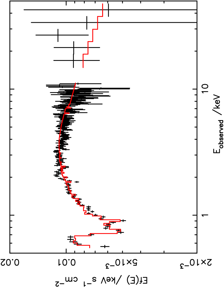
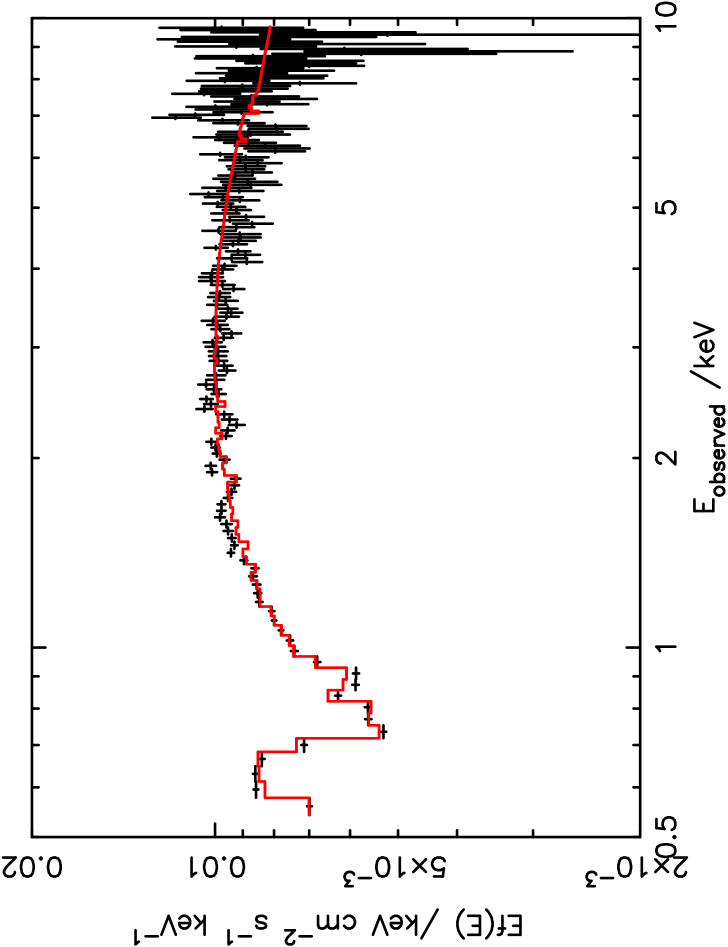
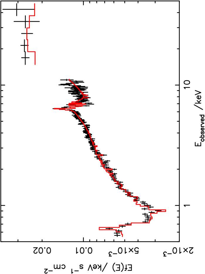
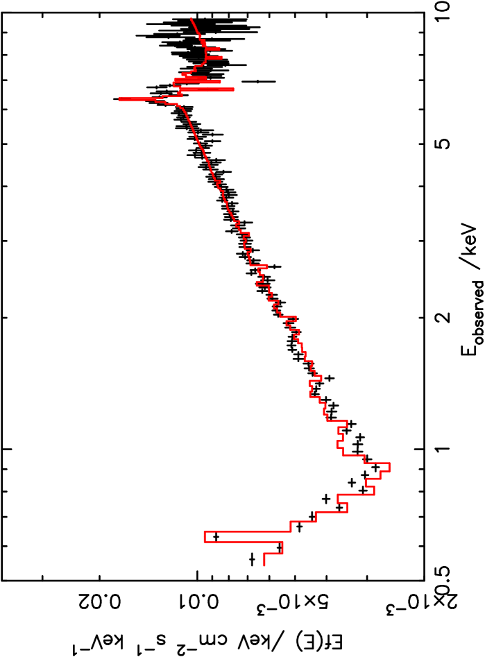
Figure 3: The fit of model B, to the principal component spectra: (left) Suzaku 0.5-45 keV, (right) XMM-Newton 0.4-10 keV; (top) eigenvector one, (bottom) offset component. The model is shown in units of Ef(E), points with error bars show the ‘unfolded’ component spectrum values.

This basic model based on the grating observations provides a qualitative fit to the principal components describing the variable spectrum of MCG–6-30-15, and indicates that the absorbed, two-component source model is a good basis for further investigation (Table 4, model A. In the results tabulated, the reflionx ionisation parameter reached its maximum allowed value in the fit. Zone 3 is assumed to absorb only the offset component in fitting to the PCA components. We do not at this stage quote statistical errors on parameter values, deferring those until the model fits to the full dataset). Eigenvector one is well-fit in both datasets, although the fit of purely absorbed low-ionisation reflection to the XMM-Newton offset component is rather poor.

One problem that has already become clear with the general problem of fitting reflection models to the Suzaku data is that if the hard component is purely reflection, its amplitude at $\sim 20$ keV requires a high reflected intensity, about three times that of the directly-viewed power-law (Ballantyne et al., 2003a; Miniutti et al., 2007). One solution to this problem is to suppose that not all the hard offset component is purely reflection, but that it actually is composed at least in part of an absorbed component. Such an absorbed component can appear in the offset component if its covering fraction is variable (see the discussion in M07 and T07) - in this case the offset component effectively represents the appearance of the source in its lowest, most covered, state. If we add an absorbed amount of the incident powerlaw onto both components (as might be required if this arises as variable partial covering), with a new absorbing zone 5, it reduces the number of degrees of freedom by four and improves $\chi^{2}$ by 199 and 386 for the Suzaku and XMM-Newton datasets, respectively (Table 5, model B): a substantial improvement over the purely absorbed reflection model. The amplitude of reflected emission is reduced accordingly, thereby decreasing the requirement for an unusually high reflected intensity. If the reflector also has an uninterrupted view of the full power-law component, this further decreases the ratio of reflected to incident light. This fit is shown in Fig. 3 for both datasets. However, eigenvector one becomes less easy to interpret in this case, as it comprises contributions from both the direct continuum and the variable-covering absorbed continuum. For a robust determination of the model parameters and for testing its goodness-of-fit it is therefore essential that we fit the model directly to the data, as in the next section.

5 Results - model fits to data

5.1 Fitting methodology and initial constraints

Fitting to the PCA components should only be considered as yielding an indication of the model components that may be required, for two reasons. First, although the offset component and eigenvector one alone provide a good description of the variable X-ray spectrum at energies above 2 keV (Tables 2, 3), more complex source behaviour is implied at softer energies. Second, there is no unique interpretation of the offset component: this component essentially describes the appearance of the source around its lowest possible flux state, and the offset component spectrum we deduce may either be pure reflection or pure absorption, for a source with a variable absorption covering fraction, or some combination of the two, as indicated by the PCA. Hence we need to test the model against the actual data. This is done in this section. Model B is summarised by Fig. 4 which shows the model fitted to the mean Suzaku spectrum as described below and showing the three emission components of the model (“direct” power-law, with ionised absorption; “partially-covered” power-law, with higher opacity absorption from zone 5; and low-ionisation reflection with absorption from zone 4). We also show the component of cosmic X-ray background emission included in the fit to hxd pin data.

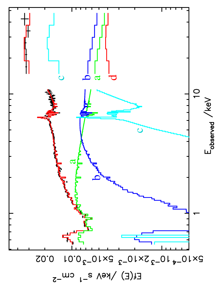
Figure 4: Illustration of the spectral model. The upper curve shows the model fitted to the mean Suzaku spectrum, with xis data below 11 keV and pin data above 15 keV. Points with error bars show the unfolded data (see section 5.3 for details). The three emission components are shown as (a) primary directly-viewed power-law, absorbed by zones 1 & 2; (b) partially-covered power-law, absorbed by zones 1, 2, 3 & 5; (c) reflection, absorbed by zones 1, 2, 3 & 4. In the fit to the PCA components, zone 3 is excluded from eigenvector one; in the fit to the actual data, zone 3 is allowed to absorb all components. Also shown is the expected contribution of the cosmic X-ray background to the Suzaku pin band (d) included in the model.

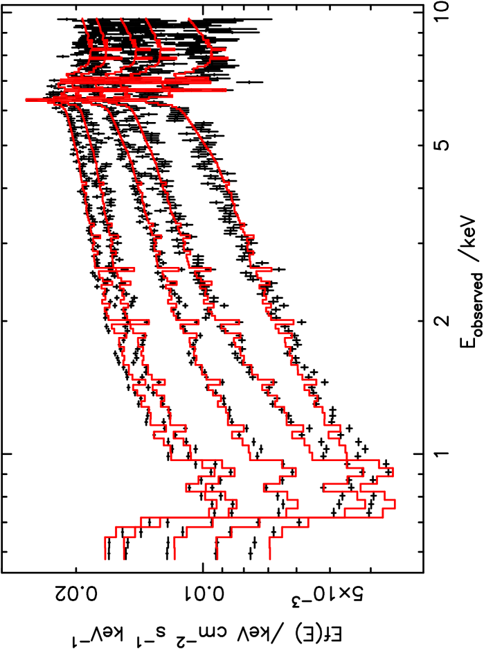
Figure 5: Simultaneous fits to the XMM-Newton data split into 5 flux states, 0.55-9.7 keV. The model is shown in units of Ef(E), points with error bars show the ‘unfolded’ data.

The full dataset that we investigate here comprises observations taken at a number of epochs with a variety of instruments. In fitting to the data we require the model to fit simultaneously any data that were obtained simultaneously (e.g. rgs and pn data for XMM-Newton or pin and xis data for Suzaku ). We do allow variations in model parameter values between datasets taken at different epochs, although the model components are not changed.

Some model components are better constrained by some datasets than others. A particular case is the high-ionisation outflowing zone 3, which is most strongly constrained by the high-resolution grating data, and in particular by the Chandra heg data around 6.7 keV (Young et al., 2005). In order to ensure that the models fitted to CCD-resolution data are consistent with the Chandra grating dataset, we first estimate parameters for zone 3 by fitting a simple model to the Chandra data that reproduces the outflowing 6.7 keV and 6.97 keV line equivalent widths and redshift. Those model parameters are then fixed in fits to the other datasets. Once the other datasets have also been fitted, the full model is then also fitted to the Chandra grating data as a final check on the model.

Because these lines are easily saturated, the equivalent widths are strongly dependent on the assumed turbulent velocity dispersion in the absorbing gas. A low turbulent velocity would require a high column, close to Compton-thick, in order to obtain the equivalent widths observed. A higher turbulent velocity dispersion would lead to line widths inconsistent with those observed (these statements were tested using xstar models created with velocity dispersion $\sigma=10,300,500,1000$ km s^-1). We use a model with $\sigma=500$ km s^-1. Thus the column and ionisation fit parameters we obtain would need to be modified if the true $\sigma$ differs from 500 km s^-1, but a comparable goodness of fit can be obtained. We find higher velocity dispersions need lower columns at fixed ionisation parameter to reproduce the observed line equivalent widths, but that higher values of ionisation parameter are needed to reproduce the 6.7, 6.97 keV line ratios. The initial absorber parameter values found from the Chandra data were $N_{\rm H}=2.1\times 10^{22}$ cm^-2, $\log\xi=3.85$ and outflow velocity 1800 km s^-1 with respect to the systemic redshift. The same value of $\xi$ and the outflow velocity were adopted when fitting to the PCA components.

In fitting to the PCA, we observed that the zone 3 absorption lines appeared only on the offset component, which implies that either (i) the absorber is only in front of the region responsible for the offset component, or (ii) the equivalent widths of the zone 3 lines decrease with increasing flux, perhaps because of increasing ionisation. The same effect is seen in Mrk 766 (T07). In fitting to the data we initially adopt the same zone 3 column and ionisation for all flux states of the source, but later we shall investigate fits in which the ionisation of zone 3 is allowed to vary between different flux states.

5.2 Fits to XMM-Newton multiple flux states

The model is now compared with the variable X-ray spectrum more directly than in the PCA, by dividing the data into a number of “flux states” each with a different spectrum, and fitting jointly to those spectra. We start with the XMM-Newton data.

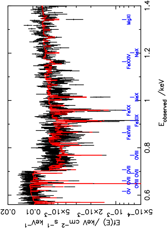
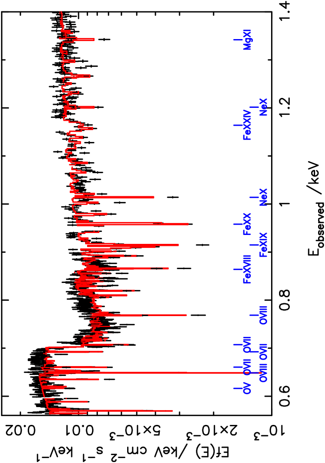
Figure 6: Fit to (left) the 2000 and (right) the 2001 XMM-Newton rgs spectra of MCG–6-30-15: The model is shown in units of Ef(E), points with error bars show the ‘unfolded’ data.

Table 6: Model parameter values for the XMM-Newton pn + rgs, Suzaku xis + pin and Chandra meg + heg fits, where $\Gamma$ is power-law photon index, $\xi$ is ionisation parameter in units of erg cm s^-1 and N_H is absorber hydrogen column density assuming solar abundances, in units of $10^{22}$ erg cm s^-1. Quoted uncertainties are 68 percent confidence intervals. Brackets indicate values that were not free parameters for that particular dataset. The final rows give goodness-of-fit: the data for each mission were jointly fit, but the contributions to $\chi^{2}$ are quoted separately for each of the subsets of XMM-Newton data: ^a pn, ^b 2001 rgs, ^c 2000 rgs (see text).

parameter	XMM-Newton		Suzaku		Chandra
$\Gamma$	2.284 $\pm$	0.013	2.265 $\pm$	0.017	(2.284)
$\log\xi_{\rm REFLIONX}$	2.04 $\pm$	0.01	1.97 $\pm$	0.03	(2.04)
NH(Gal)	0.040 $\pm$	0.004	0.052 $\pm$	0.003	0.057 $\pm$	0.002
$\tau_{\rm 0.7\,keV\,edge}$	0.42 $\pm$	0.02	0.36 $\pm$	0.03	0.45 $\pm$	0.03
NH(1)	0.26 $\pm$	0.02	0.45 $\pm$	0.05	0.11 $\pm$	0.08
$\log\xi$(1)	2.64 $\pm$	0.02	2.78 $\pm$	0.07	2.33 $\pm$	0.05
NH(2)	0.016 $\pm$	0.001	0.03 $\pm$	0.001	0.022 $\pm$	0.001
$\log\xi$(2)	0.25 $\pm$	0.08	$-0.11$ $\pm$	0.1	$-0.04$ $\pm$	0.16
NH(3)	(2.10)		(2.10)		(2.10)
$\log\xi$(3)	(3.85)		(3.85)		(3.85)
NH(4)	34.8 $\pm$	0.05	54.9 $\pm$	0.05	(34.8)
$\log\xi$(4)	1.83 $\pm$	0.01	1.94 $\pm$	0.01	(1.83)
NH(5)	5.40 $\pm$	0.08	4.32 $\pm$	0.11	(5.40)
$\log\xi$(5)	1.75 $\pm$	0.02	1.39 $\pm$	0.05	(1.75)
flux-states	$799/783^{a}$		715/841
$\chi^{2}$/dof
mean spectra	$102/159^{a}$		115/171		3406/3341
$\chi^{2}$/dof	$1965/873^{b}$
	$1820/1074^{c}$

The XMM-Newton pn data were each divided into 5 flux states, separated by equal logarithmic intervals of flux defined in the 1-2 keV band, spanning the range of flux covered by the data. These states were fit simultaneously, with a single value of parameters such as power-law index and absorber column density and ionisation parameters, with absorber properties initially chosen to match the fits to the PCA. The optical depth of the dust edge was also allowed to be a single free parameter, the same for all flux states. For each flux state, the direct, absorbed power-law and reflected component amplitudes were allowed to vary independently. Hence there were 15 free parameters, of which three were allowed to vary between flux states. We fix abundances to solar values throughout.

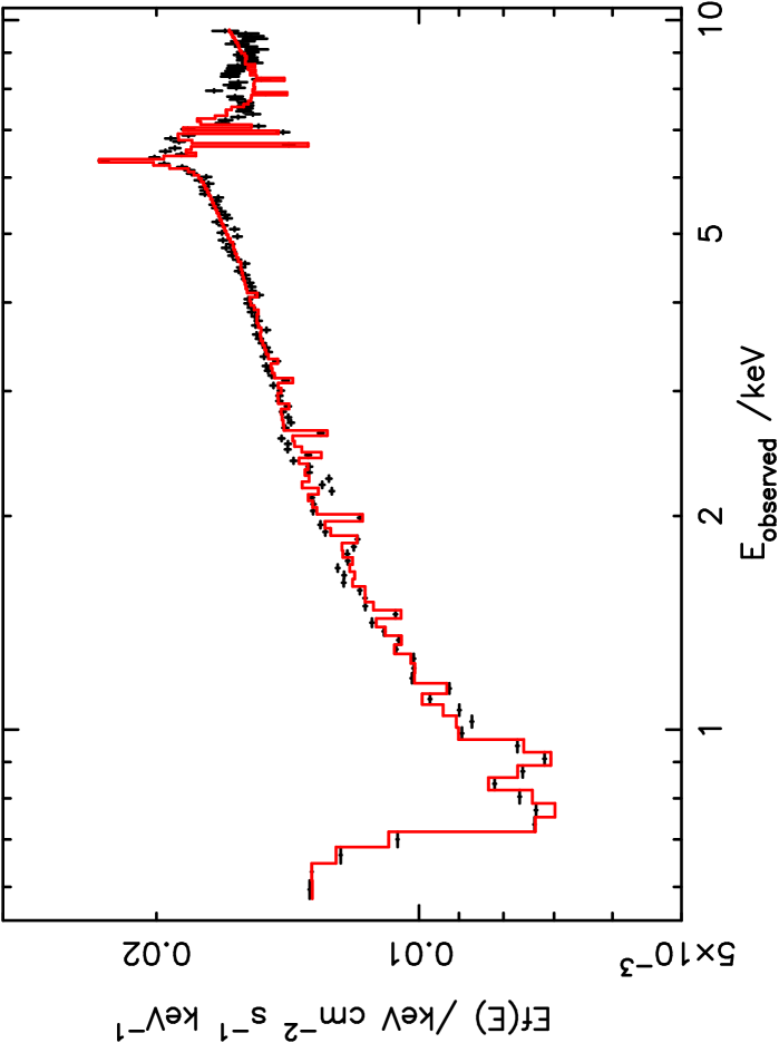
Figure 7: Fit to the mean XMM-Newton spectrum of MCG–6-30-15. The model is shown in units of Ef(E), points with error bars show the ‘unfolded’ data.

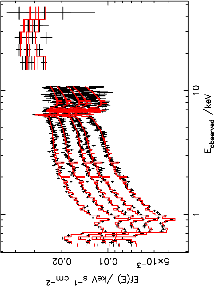
Figure 8: Simultaneous fits to the Suzaku data split into 5 flux states, 0.5-45 keV. The model is shown in units of Ef(E), points with error bars show the ‘unfolded’ data.

As discussed above, it is important to further constrain the soft-band emission from the models, to be consistent with the high-resolution grating data. The XMM-Newton observations comprised simultaneous rgs and pn observations, and hence the models were fit simultaneously to the pn flux state and the rgs data. Because of low signal-to-noise, the rgs data were not themselves divided into flux states, and the model was required to fit the mean rgs spectrum. Because of its limited energy range, the amplitudes of the various components are not well constrained by the rgs data, so as well as the individual pn flux state data, the pn mean spectrum was also included in the fit and the rgs parameters were tied to the parameters for that component. A nominal cross-calibration constant factor was allowed for each of rgs 1 and rgs 2 between the rgs and pn fits, although the value of this parameter was unity to within one percent. The 2001 rgs data are of significantly higher signal-to-noise than the 2000 data, so only the 2001 data was used to constrain the model parameters using the above procedure. Having obtained the absorber and emitter parameters, we present also the results of jointly fitting the same model to the 2000 data, with the same absorber parameters and only differing normalisations of the emission components.

This joint analysis yields an overall goodness-of-fit $\chi^{2}=2773$ for 1689 degrees of freedom. The excess in $\chi^{2}$ arises entirely in the rgs portion of the data, although the model still describes the high-resolution spectrum with an accuracy about 5 percent and correctly reproduces the chief lines and edges seen in the rgs data. The model fit to the rgs portion is discussed more below and in section 5.5.

Fig. 5 shows the fit to the pn data portion. The contribution to $\chi^{2}$ from the pn data alone is $\chi^{2}=799$ for 783 degrees of freedom (Table 6) (counting all free parameters when quoting the number of degrees of freedom). Parameter uncertainties quoted in the table are 68 percent confidence intervals. We note that this is not the best fit that can be achieved if the rgs data are ignored: but the fit to the pn data that is constrained by both pn and rgs data is nonetheless a good fit. The largest discrepancy between the pn data and the model occurs in the soft band in the lowest flux state, and likely indicates the effect of time variable absorption, which we have not taken into account in this analysis.

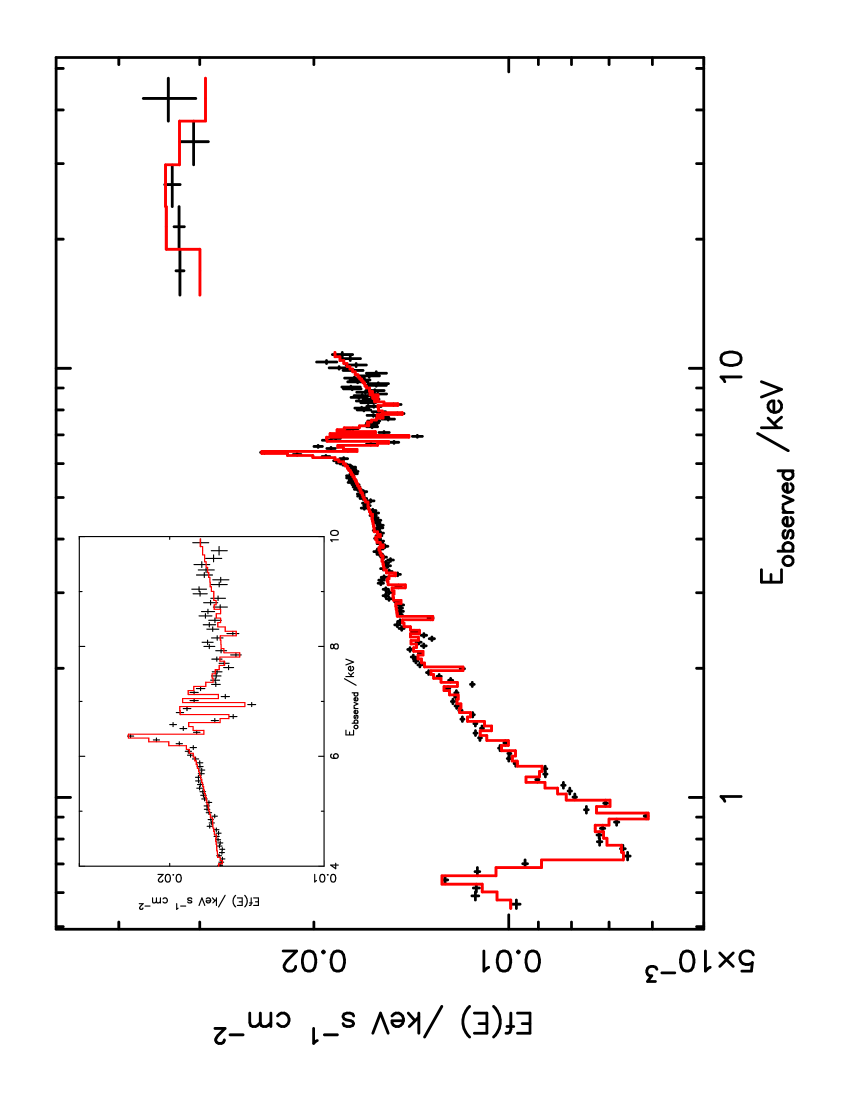
Figure 9: Fit to the mean Suzaku spectrum of MCG–6-30-15: with inset showing the zoom-in to the 4-10 keV region. The model is shown in units of Ef(E), points with error bars show the ‘unfolded’ data.

Fig. 6 shows the 2001 rgs portion of the model fit, and also shows the fit of the same model to the 2000 rgs data as mentioned above. The rgs 1 and rgs 2 data are overplotted on the figure rather than being averaged together in regions of overlap. The models fit less well than for the pn, with the rgs contribution to $\chi^{2}$ being $\chi^{2}=1965$ for 873 degrees of freedom for the 2001 data in the energy range shown, $0.56-1.4$ keV (to be conservative, again, all jointly-fit parameters are counted as being free for the calculation of the number of degrees of freedom). The 2000 data are of lower signal-to-noise and as a consequence have a better goodness-of-fit, $\chi^{2}=1820$ for 1074 degrees of freedom in the same energy range. Note that, as above, the quoted fit is not the best-fit of the model to the rgs data alone, but rather is the contribution to $\chi^{2}$ of the rgs data to the joint pn and rgs best fit, and therefore is degraded by any cross-calibration uncertainty between the two instruments. Given also the complexity of the rgs spectra and the relative simplicity of the models, including the assumption of solar abundances (section 5.5), these relatively poor rgs fits are not too surprising. The largest discrepancies between model and data in the energy range considered are at energies just above the 0.7 keV edge, and the simple, single-edge model that we have adopted is likely too simplistic. We do not have sufficient information to attempt more sophisticated models of this region. However, the reproduction of the overall continuum shape, the lack of strong emission lines and the good correspondence with the majority of the absorption features indicates that the small number of zones that have been included do account for the majority of the features. Many of the absorption lines identified by Turner et al. (2004) are reproduced by the model, adopting those authors’ line identifications we find a good match for 0.65 keV O viii Ly$\alpha$, 0.77 keV O viii Ly$\beta$, 0.87 keV Fe xviii, 0.92 keV Fe xix, 0.96 keV Fe xx, 1.02 keV Ne x Ly$\alpha$ and 1.35 keV Mg xi. These lines chiefly originate in zone 1, and some from zone 3, with zone 2 providing most of the lines and edges of O v-O vii.

We also fit the same additive model to the mean XMM-Newton spectrum where model parameters were fixed at the values found above, only allowing the normalisations of the three emission components to float. This results in a somewhat better-than-expected fit (assuming systematic fractional error 0.03), $\chi^{2}=102$ with 159 degrees of freedom (Table 6, Fig. 7), although of course the same data were used to generate the model with more free parameters when analysing the multiple flux state data above.

5.3 Fits to Suzaku multiple flux states and mean spectrum

We carry out a similar procedure for fitting to the Suzaku data, except now there is no simultaneous high resolution data, but there is simultaneous xis and pin data. The flux-state XIS data were noisy above 10.5 keV, so the XIS data were truncated at that energy. When fitting to the Suzaku pin data, the data were not corrected for the contribution of the cosmic X-ray background (CXB), but instead the CXB model adopted by Miniutti et al. (2007) was included in the fit, with a normalisation allowed to float by $\pm 5$ percent to allow for the uncertainty in the model and in the Suzaku absolute calibration.

The results are displayed in Fig. 8. Fitting to all five flux states with this model yields $\chi^{2}=715$ for 841 degrees of freedom, best-fitting parameter values are given in Table 6.

We also fit the same additive model to the mean Suzaku spectrum where again the model parameters were fixed at the values found in the flux states analysis, only allowing the normalisations of the three emission components to float. This results in goodness-of-fit $\chi^{2}=115$ for 171 degrees of freedom (Table 6, Fig. 9). An even lower value of $\chi^{2}$ may be obtained by allowing other parameters to float, but as the model would then no longer fit the variable flux state data we do not allow this freedom.

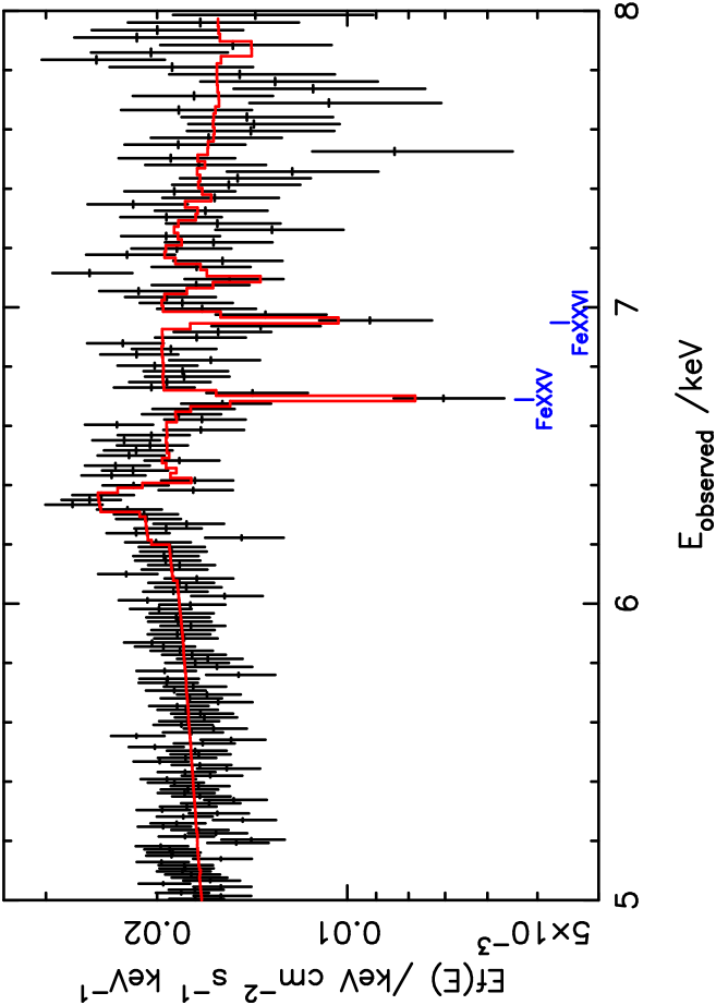
Figure 10: Model fit to Chandra heg spectrum in the region $5-8$ keV (solid line) with unfolded data shown as points with errors.

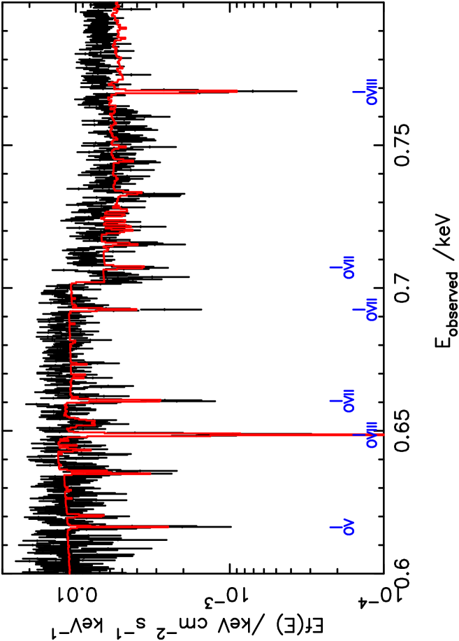
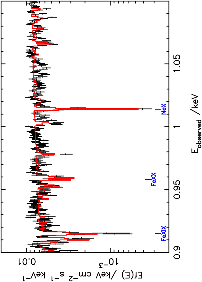
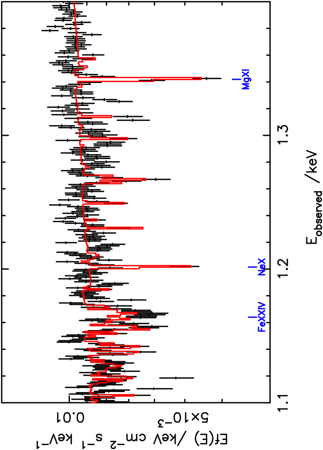
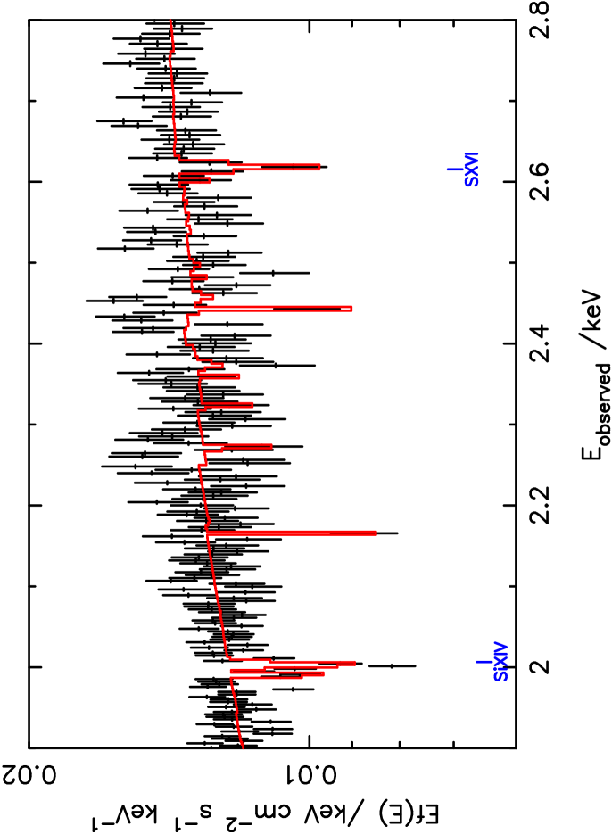
Figure 11: Model fit to the Chandra meg data, showing selected energy ranges, with the model shown as the solid line, unfolded data as points with error bars.

5.4 Fits to Chandra hetgs data

The available Chandra hetgs data has previously been analysed by Lee et al. (2001) and Young et al. (2005) who have demonstrated its diagnostic power in detecting the presence of absorbing layers. The data were taken at a different epoch from the XMM-Newton and Suzaku data, with a different instrument, and so we expect to need to vary some of the parameters in order to obtain a good fit. The mean heg spectrum over the range $3-8$ keV and the mean meg spectrum over the range $0.55-5$ keV were jointly fit with the same model as the other datasets, with free parameters as before, except that the power-law slope, reflionx ionisation parameter and some absorption zones were fixed at the XMM-Newton values (see Table 6; the mean Chandra spectrum on its own does not sufficiently constrain these parameters). The resulting parameter values are shown in Table 6, which resulted in a goodness-of-fit $\chi^{2}=3406$ for 3341 degrees of freedom for the joint fit.

Viewing the fit in more detail, we first consider the heg data in the region around 7 keV. The pair of absorption lines at this energy have already been discussed in this paper and by Young et al. (2005); Brenneman & Reynolds (2006) and Miniutti et al. (2007). Fig. 10 shows the model fitted to the data, and it can be seen both that the absorption lines are reproduced by this model and that no other strong lines are expected, and it is therefore consistent with the constraint discussed by Young et al. (2005) that there should not be significant amounts of absorption from intermediate ionisation states of Fe, which would produce absorption at $\sim 6.5$ keV. This constraint is avoided because the red wing is largely produced by zone 5, which has ionisation sufficiently low that the Fe L shell is filled, at $\log\xi\la 2$ (Kallman et al., 2004), and it is the partial covering of this zone that allows the continuum shape to be correctly reproduced as well as explaining the variability properties (discussed further in section 6.2).

Further confirmation of the high-ionisation layer comes from the Chandra meg data, in which numerous absorption features arising in this layer are visible, including the features at 2.0 and 2.62 keV discussed by Young et al. (2005) (Fig. 11).

As in the rgs data, the meg data reveal numerous absorption lines in the soft band, many of which were previously identified by Lee et al. (2001) and Turner et al. (2004), including 0.615 keV O v, 0.635 keV O vi, 0.66 keV and 0.69 keV O vii, 0.65 keV O viii Ly$\alpha$, 0.77 keV O viii Ly$\beta$, 0.92 keV Fe xix, 1.02 keV Ne x Ly$\alpha$, 1.35 keV Mg xi and 2.0 keV Si xiv Ly$\alpha$ (we again adopt the line identifications of Lee et al. (2001) and Turner et al. (2004)). Again, the higher ionisation lines chiefly originate in zones 1 and 3, the lower ionisation lines in zone 2.

5.5 The effect of non-solar abundances

In the above models, solar abundances were assumed throughout. However, there is evidence in MCG–6-30-15 for departures from those values: Turner et al. (2004) point out that the observed equivalent widths of absorption lines in their model are too low by a factor $\sim 1.25$, an effect that is also clearly seen in the fits shown here (e.g. Fig. 6). The effect could be explained either by altering the assumed velocity dispersion, or by altering the assuming abundance.Clearly, allowing either of these parameters to float would result in an overall goodness of fit better than presented here. Because of the degeneracies in such fits with other parameters, not only velocity dispersion but also column density and ionisation parameter, the current data is insufficient to unambiguously determine absolute values of element abundances. We can, however, estimate the size of the effect of changing the assumed abundance to an alternate value. Turner et al. (2004) suggest O may need to be enhanced by a substantial factor, perhaps as high as $3-4$, to explain the observed equivalent widths. We have therefore replaced the absorber model used for zone 1 with a new xstar model with $\alpha$-element abundance enhanced by a factor two, leaving other abundances fixed at solar. Consistent with the inference of Turner et al. (2004), we find an improved overall fit to the XMM-Newton combined pn/2001 rgs data. The overall $\chi^{2}$ for the combined fit shows a modest improvement by $\Delta\chi^{2}=39$, from a value 2773 to 2734 (with 1689 degrees of freedom in both cases). As expected, the equivalent widths of the O, Ne and Mg lines match better to the data, but the Fe lines remain with model equivalent widths that are too small. It seems likely therefore that there is an overall enhancement of all elements, not only the $\alpha$ elements.

The chief aim of this paper is to investigate the extent to which an absorption model can describe the full X-ray spectrum of MCG–6-30-15. In order not to confuse the general properties of the absorption model with specific details about the likely element abundances, we do not here investigate further the more detailed effect of non-solar abundances.

5.6 Variation in absorber ionisation

We can also test the absorber models for possible variation in ionisation parameter with flux. There is evidence for this in the high ionisation outflow, zone 3, in that the equivalent width of the absorption lines decrease with increasing source brightness (equivalently, they only appear on the PCA offset component, and not on eigenvector one). This might arise if the zone 3 absorber is localised to the region responsible for the offset component, but the alternative explanation investigated here is that the variation in equivalent width is an effect of varying ionisation. Fig. 12 shows the variation in $\xi$ for each of the five XMM-Newton and Suzaku flux states when this is allowed to vary between each state. The goodness-of-fit improves by $\Delta\chi^{2}=15$ to $\chi^{2}=822$ for 838 degrees of freedom: in itself this is a weak return for introducing a further four free parameters, but it does reveal the expected relationship between ionisation and flux. Within each dataset there is a clear trend for $\xi$ to be proportional to the continuum amplitude, although the Suzaku points appear offset to lower ionisation, implying a change in either absorber density or ionising continuum spectrum between 2001 and 2006.

6 Discussion

6.1 Model complexity and uniqueness

The model presented above provides a good description of the variable X-ray spectrum of MCG–6-30-15 throughout all its flux states, and correctly reproduces the hard low-state and softer high-state spectra. It also reproduces the high energy $15-40$ keV flux and its relative lack of variability, and removes the requirement for an unexpectedly high reflection albedo. The model is complex, requiring five intrinsic absorption zones, plus a dust edge, but we know already from the Chandra and XMM-Newton grating data that multiple zones covering a wide range of ionisation, with at least two kinematically distinct regions, are required by the data. We should not be surprised by the complexity of the model, three of the zones have been detected by previous authors, but of course the next step in proving or disproving the specific model presented here would be to search for high resolution signatures of the additional heavy absorbing zones that are required. For the ionisation predicted from the model in this paper, there may be a weak signature of the Fe K$\beta$ UTA arising from ionisation states less ionised that Fe xvii. This would be too weak to detect in the present data but may be a detectable signature in data from future missions with calorimeter detectors.

We might compare the model complexity with other studies: (Brenneman & Reynolds, 2006), for example, fit the spectrum expected from close to a Kerr black hole to the XMM-Newton data for MCG$-6$-30-15, including some of the ionised absorbing zones and the dust edge, over the range $0.6-10$ keV, but only fitting the mean spectrum. That model does not include all the ionised zones seen with Chandra , but still has a total of 18 parameters, of which eight are associated with the relativistically blurred line component, and their model 4 results in a goodness-of-fit $\chi^{2}=1742$ for 1375 degrees of freedom. It seems that whatever physical premise is taken for the origin of the red wing, models of some complexity are needed.

Conversely, although the absorption model presented here has been successful, we cannot claim that it is unique. In this paper we have concentrated on a model in which absorption plays a dominant role, and have developed the model constituents in a systematic manner based on fits to the variable-spectrum low resolution data and the high-resolution grating data. This exercise at least shows that it is possible to explain the X-ray spectrum of MCG–6-30-15 by such a model. Many previous studies have concentrated solely on modelling the hard, low-variability “offset” component as being relativistically-blurred reflected emission from the inner accretion disc (Wilms et al. 2001, Vaughan & Fabian 2004, Reynolds et al. 2004, Miniutti et al. 2007, Brenneman & Reynolds 2006), but those studies have only tested that model against the mean spectra, albeit of data obtained when the source was in differing flux states, and often over a restricted range in energy (e.g., $3-45$ keV in the study of Miniutti et al. 2007). The model presented in this paper does not have any such blurred component, but this does not prove that such a component does not exist. After all, an arbitrarily low amplitude of such a component could always be added into the model described in this paper. Nonetheless, the model-fitting presented here does show that the offset component need not be considered as being dominated by relativistically-blurred reflection. One important consequence is that it is not possible to use the spectral shape of the red wing in the current generation of data to deduce parameters such as black hole spin. Given the extreme spin parameters that are deduced for AGN such as MCG$-6$-30-15 (in this case $a=0.989_{-.002}^{+.009}$, Brenneman & Reynolds 2006) this has important consequences for models of black hole evolution, as “chaotic” mergers produce lower expected spin parameter values, and such extreme high values are expected only to be achieved by long-lived steady accretion (Berti & Volonteri, 2008; King et al., 2008).

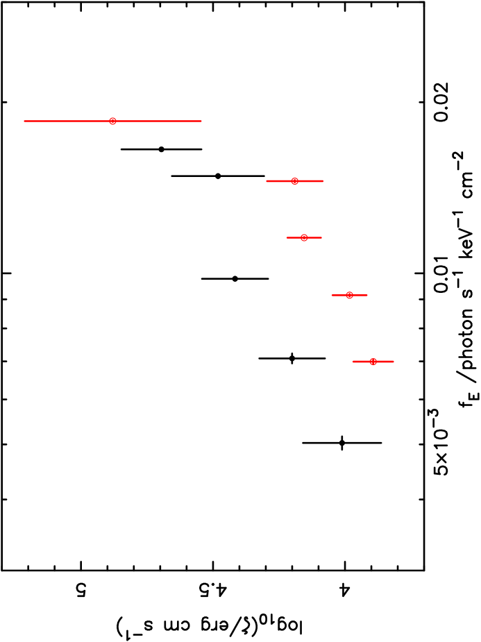
Figure 12: The fitted variation in $\xi$ as a function of normalisation of the primary power-law, for the XMM-Newton (solid points) and Suzaku (open points) flux-states.

6.2 The role of absorber partial covering

The absorbed power-law component that forms part of the model presented here is key to both understanding the soft-band continuum shape and the high flux observed in the pin data at high energy.

Many previous authors have suggested that absorption partially covers an X-ray source and that variations in covering fraction of an absorbing zone may be linked to flux and spectral variations in both AGN and Galactic black hole systems (e.g. Holt et al., 1980; Reichert et al., 1985; Boller et al., 2002, 2003; Immler et al., 2003; Tanaka et al., 2004; Gallo et al., 2004a, b; Pounds et al., 2004; Turner et al., 2005; Grupe et al., 2007, inter alia). Vaughan & Fabian (2004) previously tested a partial covering model for the 2001 XMM-Newton spectrum of MCG$-6$-30-15 and concluded that, although such a model provided an acceptable fit, a relativistically-blurred model was superior. The model tested in that case was solely a neutral absorber however, a key difference with the models tested here. McKernan & Yaqoob (1998) also suggested specifically for MCG–6-30-15 that a sharp dip in flux was caused by occultation by an absorber, an idea revived most recently for NGC 3516 by Turner et al. (2008). Mrk 766 shows extremely similar X-ray spectral variability to MCG–6-30-15 and M07 and T07 have suggested that variable partial covering may play an important or perhaps even dominant role in the X-ray spectral variability of this source.

To investigate this further we show in Fig. 13 the amplitude in the absorbed component compared with the amplitude in the direct component, as measured from the normalisation of the power-law in each case. It may be seen that, in the model presented here, the absorbed component does vary coherently with the direct continuum at high flux states, but not with a dependence that passes through the origin. We can see from this diagram why the PCA results in an offset component that contains a signficant amount of absorbed continuum: a linear extrapolation through the points in Fig. 13 would hit the y-axis at a positive value of the absorbed component flux. At the lowest observed fluxes, the correlation seems to break down, with a larger scatter in the two components. The simplest interpretation of the observed trends is that in the highest flux states the source has a covering fraction around 50 percent, but that at lower flux states the covering fraction is more variable and may increase towards 100 percent. If this interpretation is correct it implies that the covering fraction is a function of the flux state of the source and perhaps indicates a dependence of either source size or absorber extent on flux state. The trends seen here and the interpretation is however model dependent, and at this stage we can do no more than suggest this interpretation.

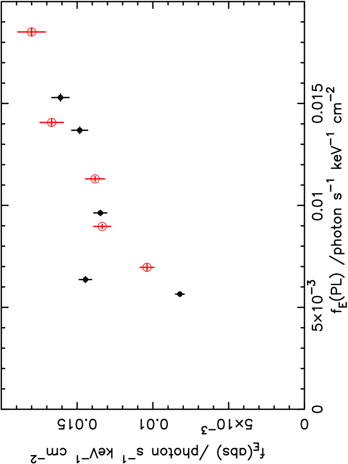
Figure 13: The variation in amplitude of the absorbed component (y-axis) as a function of the amplitude of the direct power-law component (x-axis), for the fits to the Suzaku (open symbols) and XMM-Newton (solid symbols) data.

6.3 Hard-band reflection

A problem that any model must address is the relatively high flux observed above 20 keV (Ballantyne et al., 2003a; Miniutti et al., 2007). In the model presented here, some fraction of the hard-band flux is still provided by distant reflection. If that reflection has a view of the entire unabsorbed source output, then the reflected intensity relative to that expected from a disc subtending 2$\pi$ sr (the “R” parameter) has a value around 1.7 (estimated as in Miniutti et al. 2007 from a comparison of component fluxes in the hard band): still greater than unity but substantially smaller than $R\ga 3$ as required by the previous work. In fact, almost any amount of hard-band flux could be obtained if there are further even more opaque partial covering layers or heavily-absorbed reflection zones, and recently the source PDS 456 has been found to exhibit just such a heavily absorbed zone (Reeves et al. in preparation). If the narrow Fe K$\alpha$ emission line originates in optically thin gas rather than optically-thick reflection, it may even be the case that the heavily absorbed reflection component could be largely replaced by further high-opacity partial covering layers. We do not explore such models further in this paper.

6.4 The location of the Fe emission-line region

A number of previous authors have suggested using the width of the narrow 6.4 keV Fe K$\alpha$ emission line to give an indication of its origin (Lee et al., 2002; Yaqoob & Padmanabhan, 2004). In addition to the red wing, there appears to be a resolved 6.4 keV Fe K$\alpha$ line whose width, if interpreted as due to Doppler broadening, is FWHM$\sim 10,000$ km s^-1. In the model presented here, some of this width is provided by a Compton shoulder on the line in a moderately ionised reflector, modelled by reflionx, although there may still be some residual excess emission on the blue side of the line. In this case it is difficult to disentangle Compton broadening from velocity broadening and the line width gives no clear indication of the location of the reflection, other than not being close to the black hole. If the line instead is emitted from optically-thin gas, the linewidth may indicate an origin in the broad line region. In addition to this component, the long Chandra exposure reveals the presence of a weak (equivalent width $\sim 20$ eV) line unresolved at the heg resolution (FWHM $<3000$ km s^-1) that may indicate a further component of reflection or emission even more distant from the central source.

6.5 The location of the absorbers, rapid variability and time delays

The analysis presented here has only dealt with variability on timescales $\ga 20$ ks. Within the model presented, there is no requirement for any material within radii where relativistic blurring is significant ($\la 20$ r_g) but we suggest that the heavy partial-covering absorbing layer originates on scales of the accretion disc, perhaps around 100 r_g. Perhaps the most compelling evidence for this is the observation of an apparent eclipse-like event in the light curve of MCG$-6$-30-15 (McKernan & Yaqoob, 1998) which may be explained as a clumpy disc wind occulting part of the source. M07 and T07 also suggested absorption by a clumpy disc wind in Mrk 766 and a similar eclipse event to that seen in MCG$-6$-30-15 has been observed in NGC 3516 (Turner et al., 2008). Full spectral models of such a wind do not currently exist, although Schurch & Done (2007) have created approximate spectra by layering (1D) xstar absorption zones and Sim et al. (2008) are developing steady axisymmetric wind models based on Monte-Carlo radiative transfer that qualitatively reproduce many of the features seen in AGN and Galactic black hole binary system X-ray spectra. Dorodnitsyn et al. (2008) have calculated transmission spectra in a time-dependent axisymmetric model of parsec-scale flows in AGN. We can hope that detailed comparison of observed spectra with realistic wind models will become possible in the near future.

In the model presented here there is also a component of low-ionisation reflection. the amplitude of this is so constant that it is very likely from distant material, light-days or further away, with any reflection variability erased by light travel time delays. However, Ponti et al. (2004) have found evidence for a transient reflection signal delayed after a continuum flare by a few ks. The statistical significance of the delayed flare is low and needs to be confirmed by detection of further similar events. Goosmann et al. (2007) have modelled the phenomenon as reflection from a dense clumpy medium surrounding the accretion region at $\sim 70$ r_g. If our hypothesised absorbing clumpy disk wind is present, we might expect to see some reflection contribution from it, depending on its scattering optical depth and covering factor. We suggest that the clumpy disc wind may also be visible in reflection on short-lived occasions after a flare when viewed with adequate time resolution. On the 20 ks timescales used in the analysis in this paper such reflection, weak in normal circumstances, would simply be included as an additional component in the variable component of the spectrum (PCA eigenvector one).

We may also be able to constrain the location of the absorbing zones from their response, or lack of, to the continuum variations. Of the various zones, only the high ionisation outflow, zone 3, seems to show evidence for ionisation variation that tracks the continuum brightness (section 5.6). This interpretation of the change in equivalent width is not unique, it could also arise if zone 3 were only associated with the heavily-absorbed components, but if the ionisation-variation interpretation is correct it implies that the recombination time in the absorbing zone is no larger than the typical continuum variability timescale, and in turn that the depth of the zone should be $\la 10$ light days, assuming a Fe xxvi radiative recombination rate coefficient $\alpha\simeq 10^{-11}$ cm³ s^-1 (Shull & Van Steenberg, 1982). This might place the wind within the broad-line region. In the other absorbing zones that are detected in the grating data, there do also appear to be ionisation variations, but these do not appear to be systematically correlated with the source brightness (Gibson et al., 2007), which might imply that their densities are rather low, or else that more complex radiative transfer is present. There is currently no constraint on ionisation variation of the heavily absorbing zones 4 and 5.

6.6 Comparison with other AGN

Much of the analysis in this paper has followed that carried out for Mrk 766, a narrow-line Seyfert I, by M07 and T07. There are strong similarities between the X-ray spectra of the two sources:

1. Both sources show similar systematic variation in spectral shape with flux on 20 ks timescales, with a hard component in the low flux state that shows a significant edge around the Fe K$\alpha$ region.

2. The PCA leads to similar spectral components in both sources, with the “red wing” component being dominated by an apparently quasi-constant hard spectral component.

3. Both sources appear to have absorption from a high-ionisation outflow, which leads to significant modification of the observed spectral shape around 7 keV.

4. The soft excess appears to be explained by ionised absorption.

The implication is that MCG$-6$-30-15 is not a special case, but that it is a examplar of a general class of AGN whose X-ray spectra are dominated by the effects of absorption, possibly in an outflowing wind. Nandra et al. (2007) have attempted to quantify the occurrence of “red wings” in AGN, with the aim of establishing the prevalence of detectable relativistic blurring. They find that 45 percent of AGN in their sample are best fit by a relativistically blurred component, including MCG$-6$-30-15 and Mrk 766. The results we obtain suggest that a partial covering model such as presented here would provide an alternative explanation of the observed red wings in AGN. The high occurrence rate in the Nandra et al. (2007) sample would then imply a high prevalence of significant wind absorption, that in turn would imply a high global covering fraction for the wind. If the wind explanation is correct, the inference of X-ray winds in the detailed studies of three AGN, Mrk 766, MCG$-6$-30-15 and NGC 3516 (Turner et al., 2008), would require that the phenomenon be a property of sources across the range of narrow-line Seyfert I and broad-line Seyfert I AGN characteristics, across a range of black hole mass, as indicated by the wide range of sources for which a red wing is claimed in the Nandra et al. study.

7 Conclusions

We have investigated a model of X-ray spectral variability for MCG$-6$-30-15 based on the absorbing zones identified in high-resolution grating data. We find the “soft excess” may be explained entirely by the combined effect of those zones (including soft-band dust absorption). High-resolution principal components analysis, achieved using singular value decomposition, indicates the presence of a less variable heavily absorbed component that until now has been interpreted as a relativistically-blurred Fe line. This component may be modelled by a combination of distant (constant amplitude) absorbed reflection and the effect of a variable covering fraction of absorption of the primary continuum source. The model has been applied both to the PCA and the actual data accumulated from the XMM-Newton pn and rgs instruments (simultaneously-fitted) in 2000 and 2001 over the energy range $0.5-10$ keV, to the Suzaku xis, $0.5-10.5$ keV, and pin, $15-45$ keV, data (simultaneously fitted) from 2006 and to the Chandra hetgs data (heg and meg simultaneously fitted) from 2004. This is the most comprehensive analysis of the MCG$-6$-30-15 dataset yet published. Remarkably, the absorption model fits the entire dataset over its entire range, explaining simultaneously the soft-band excess, the “red wing” and its lack of variability and the high hard band (BeppoSAX and Suzaku pin) flux and its lack of variability, and fits not only the CCD-resolution data but also matches well the absorption lines and edges seen in the high resolution grating data. The best-fit parameters show that the partial-covering absorber is ionised, but with $\xi<100$ erg cm s^-1, so no Fe K$\alpha$ absorption is expected from this component, and the absence of observed 6.5 keV Fe K$\alpha$ absorption (Young et al., 2005) is not therefore a constraint on this model. No relativistically blurred component is required to fit this dataset. We suggest the absorbing material is primarily a clumpy disc wind.