Maximal Orders in the Design of Dense Space-Time Lattice Codes

Abstract

We construct explicit rate-one, full-diversity, geometrically dense matrix lattices with large, non-vanishing determinants (NVD) for four transmit antenna multiple-input single-output (MISO) space-time (ST) applications. The constructions are based on the theory of rings of algebraic integers and related subrings of the Hamiltonian quaternions and can be extended to a larger number of Tx antennas. The usage of ideals guarantees a non-vanishing determinant larger than one and an easy way to present the exact proofs for the minimum determinants. The idea of finding denser sublattices within a given division algebra is then generalized to a multiple-input multiple-output (MIMO) case with an arbitrary number of Tx antennas by using the theory of cyclic division algebras (CDA) and maximal orders. It is also shown that the explicit constructions in this paper all have a simple decoding method based on sphere decoding. Related to the decoding complexity, the notion of sensitivity is introduced, and experimental evidence indicating a connection between sensitivity, decoding complexity and performance is provided. Simulations in a quasi-static Rayleigh fading channel show that our dense quaternionic constructions outperform both the earlier rectangular lattices and the rotated ABBA lattice as well as the DAST lattice. We also show that our quaternionic lattice is better than the DAST lattice in terms of the diversity-multiplexing gain tradeoff.

I Introduction and background

Multiple-antenna wireless communication promises very high data rates, in particular when we have perfect channel state information (CSI) available at the receiver. In [1] the design criteria for such systems were developed and further on the evolution of ST codes took two directions: trellis codes and block codes. Our work concentrates on the latter branch.

The very first ST block code for two transmit antennas was the Alamouti code [2] representing multiplication in the ring of quaternions. As the quaternions form a division algebra, such matrices must be invertible, i.e. the resulting STBC meets the rank criterion. Matrix representations of other division algebras have been proposed as STBCs at least in [3]-[15], and (though without explicitly saying so) [16]. The most recent work [6]-[16] has concentrated on adding multiplexing gain, i.e. multiple input-multiple output (MIMO) applications, and/or combining it with a good minimum determinant. In this work, we do not specifically seek any multiplexing gains, but want to improve upon e.g. the diagonal algebraic space time (DAST) lattices introduced in [5] by using non-commutative division algebras. Other efforts to improve the DAST lattices and ideas alike can be found in [17]-[19].

The main contributions of this work are:

• We give energy efficient MISO lattice codes with simple decoding that win over e.g. the rotated ABBA [20] and the DAST lattice codes in terms of the block error rate (BLER) performance.

• It is shown that by using a non-rectangular lattice one can gain major energy savings without significant increasement in decoding complexity. The usage of ideals moreover guarantees a non-vanishing determinant $>1$ and an easy way to present the exact proofs for the minimum determinants.

• In addition to the explicit MISO constructions, we present a general method for finding dense sublattices within a given CDA in a MIMO setting. This is tempting as it has been shown in [15] that CDA-based square ST codes with NVD achieve the diversity-multiplexing gain tradeoff (DMT) introduced in [21]. When a CDA is chosen the next step is to choose a corresponding lattice or, what amounts to the same thing, choose an order within the algebra. Most authors, among which e.g. [11], [15], and [16], have gone with the so-called natural order (see Section III-B, Example III.2). In a CDA based construction, the density of a sublattice is lumped together with the concept of maximality of an order. The idea is that one can, on some occasions, use several cosets of the natural order without sacrificing anything in terms of the minimum determinant. So the study of maximal orders is easily motivated by an analogy from the theory of error correcting codes: why one would use a particular code of a given minimum distance and length, if a larger code with the same parameters is available.

• Furthermore, related to the decoding complexity, the notion of sensitivity is introduced for the first time, and evidence of its practical appearance is provided. Also the DMT behavior of our codes will be given.

At first, we are interested in the coherent MISO case with perfect CSI available at the receiver. The received signal $\mathbf{y}\in\mathbb{C}^{n}$ has the form

$$\mathbf{y}=\mathbf{h}X+\mathbf{n},$$

where $X\in\mathbb{C}^{m\times n}$ is the transmitted codeword drawn from a ST code $\mathcal{C}$, $\mathbf{h}\in\mathbb{C}^{m}$ is the Rayleigh fading channel response and the components of the noise vector $\mathbf{n}\in\mathbb{C}^{n}$ are i.i.d. complex Gaussian random variables.

A lattice is a discrete finitely generated free abelian subgroup of a real or complex finite dimensional vector space $V$, also called the ambient space. Thus, if $L$ is a $k$-dimensional lattice, there exists a finite set of vectors ${\cal B}=\{\mathbf{b}_{1},\mathbf{b}_{2},\ldots,\mathbf{b}_{k}\}\subset V$ such that ${\cal B}$ is linearly independent over the integers and that

$$L=\{\sum_{i=1}^{k}z_{i}\mathbf{b}_{i}\mid z_{i}\in\mathbb{Z},\mathbf{b_{i}}\in V\ \textrm{for all }i=1,2,\ldots,k\}.$$

In the space-time setting a natural ambient space is the space $\mathbb{C}^{n\times n}$ of complex $n\times n$ matrices. When a code is a subset of a lattice $L$ in this ambient space, the rank criterion [22] states that any non-zero matrix in $L$ must be invertible. This follows from the fact that the difference of any two matrices from $L$ is again in $L$.

The receiver and the decoder, however, (recall that we work in the MISO setting) observe vector lattices instead of matrix lattices. When the channel state is $\mathbf{h}$, the receiver expects to see the lattice $\mathbf{h}L$. If $\mathbf{h}\neq 0$ and $L$ meets the rank criterion, then $\mathbf{h}L$ is, indeed, a free abelian group of the same rank as $L$. However, it is well possible that $\mathbf{h}L$ is not a lattice, as its generators may be linearly dependent over the reals — the lattice is said to collapse, whenever this happens.

From the pairwise error probability (PEP) point of view [22], the performance of a space-time code is dependent on two parameters: diversity gain and coding gain. Diversity gain is the minimum of the rank of the difference matrix $X-X^{\prime}$ taken over all distinct code matrices $X,X^{\prime}\in\mathcal{C}$, also called the rank of the code $\mathcal{C}$. When $\mathcal{C}$ is full-rank, the coding gain is proportional to the determinant of the matrix $(X-X^{\prime})(X-X^{\prime})^{H}$, where $X^{H}$ denotes the transpose conjugate of the matrix $X$. The minimum of this determinant taken over all distinct code matrices is called the minimum determinant of the code $\mathcal{C}$ and denoted by $\delta_{\mathcal{C}}$. If $\delta_{\mathcal{C}}$ is bounded away from zero even in the limit as SNR $\rightarrow\infty$, the ST code is said to have the non-vanishing determinant property [8]. As mentioned above, for non-zero square matrices being full-rank coincides with being invertible.

The data rate $R$ in symbols per channel use is given by

$$R=\frac{1}{n}\textrm{log}_{|S|}(|\mathcal{C}|),$$

where $|S|$ and $|\mathcal{C}|$ are the sizes of the symbol set and code respectively. This is not to be confused with the rate of a code design (shortly, code rate) defined as the ratio of the number of transmitted information symbols to the decoding delay (equivalently, block length) of these symbols at the receiver for any given number of transmit antennas using any complex signal constellations. If this ratio is equal to the delay, the code is said to have full rate.

The correspondence is organized as follows: basic definitions of algebraic number theory and explicit MISO lattice constructions are provided in Section II. As a (MIMO) generalization for the idea of finding denser lattices within a given division algebra, the theory of cyclic algebras and maximal orders is briefly introduced in Section III. In Section IV, we consider the decoding of the nested sequence of quaternionic lattices from Section II. A variety of results on decoding complexity is established in Section IV, where also the notion of sensitivity is taken into account. Simulation results are discussed in Section V along with energy considerations. Finally in Section VI, the DMT analysis of the proposed codes will be given.

This work has been partly published in a conference, see [3] and [4]. For more background we refer to [22]-[29].

II Rings of algebraic numbers, quaternions and lattice constructions

We shall denote the sets of integers, rationals, reals, and complex numbers by $\mathbb{Z},\ \mathbb{Q},\ \mathbb{R}$, and $\mathbb{C}$ respectively.

Let us recall the set

$$\mathbb{H}=\{a_{1}+a_{2}i+a_{3}j+a_{4}k\mid a_{t}\in\mathbb{R}\ \forall t\},$$

where $i^{2}=j^{2}=k^{2}=-1,\ ij=k$, as the ring of Hamiltonian quaternions. Note that $\mathbb{H}\simeq\mathbb{C}\oplus\mathbb{C}j$, when the imaginary unit is identified with $i$. A special interest lies on the subsets

$$\mathbb{H}_{\mathcal{L}}=\{a_{1}+a_{2}i+a_{3}j+a_{4}k\mid a_{t}\in\mathbb{Z}\ \forall t\}\subseteq\mathbb{H}\ \textrm{and}$$

$$\mathbb{H}_{\mathcal{H}}=\{a_{1}\rho+a_{2}i+a_{3}j+a_{4}k\mid a_{t}\in\mathbb{Z}\ \forall t,\ \rho=\textrm{\textonehalf}(1+i+j+k)\}\subseteq\mathbb{H}$$

called the Lipschitz’ and Hurwitz’ integral quaternions respectively.

We shall use extension rings of the Gaussian integers

$${\cal G}=\{a+bi\mid a,b\in\mathbb{Z}\}$$

inside a given division algebra. It would be easy to adapt the construction to use the slightly denser hexagonal ring of the Eisensteinian integers

$${\cal E}=\{a+b\omega\mid a,b\in\mathbb{Z}\},$$

where $\omega^{3}=1$, as a basic alphabet. However, the Gaussian integers nicely fit with the popular 16-QAM and QPSK alphabets. Natural examples of such rings are the rings of algebraic integers inside an extension field of the quotient fields of ${\cal G}$, as well as their counterparts inside the quaternions. To that end we need division algebras ${\cal A}$ that are also 4-dimensional vectors spaces over the field $\mathbb{Q}(i)$.

II-A Base lattice constructions

Let now $\zeta=e^{\pi i/8}$ (resp. $\xi=e^{\pi i/4}=(1+i)/\sqrt{2}$) be a primitive $16^{th}$ (resp. $8^{th}$) root of unity. Our main examples of suitable division algebras are the number field

$$\mathbf{L}=\mathbb{Q}(\zeta),$$

and the following subskewfield

$${\bf H}=\mathbb{Q}(\xi)\oplus j\mathbb{Q}(\xi)\subseteq\mathbb{H}$$

of the Hamiltonian quaternions. Note that as $zj=jz^{*}$ for all complex numbers $z$, and as the field $\mathbb{Q}(\xi)$ is stable under the usual complex conjugation $(^{*})$, the set ${\bf H}$ is, indeed, a subskewfield of the quaternions.

As always, multiplication (from the left) by a non-zero element of a division algebra ${\cal A}$ is an invertible $\mathbb{Q}(i)$-linear mapping (with $\mathbb{Q}(i)$ acting from the right). Therefore its matrix with respect to a chosen $\mathbb{Q}(i)$-basis ${\cal B}$ of ${\cal A}$ is also invertible. Our example division algebras $\mathbf{L}$ and ${\bf H}$ have the sets ${\cal B}_{L}=\{1,\zeta,\zeta^{2},\zeta^{3}\}$ and ${\cal B}_{H}=\{1,\xi,j,j\xi\}$ as natural $\mathbb{Q}(i)$-bases. Thus we immediately arrive at the following matrix representations of our division algebras.

Proposition II.1

Let the variables $c_{1},c_{2},c_{3},c_{4}$ range over all the elements of $\mathbb{Q}(i)$. The division algebras $\bf{L}$ and ${\bf H}$ can be identified via an isomorphism $\phi$ with the following rings of matrices

$$\mathbf{L}=\left\{M_{L}=M_{L}(c_{1},c_{2},c_{3},c_{4})=\left(\begin{array}[]{rrrr}c_{1}&ic_{4}&ic_{3}&ic_{2}\\ c_{2}&c_{1}&ic_{4}&ic_{3}\\ c_{3}&c_{2}&c_{1}&ic_{4}\\ c_{4}&c_{3}&c_{2}&c_{1}\\ \end{array}\right)\right\}$$

and

$${\bf H}=\left\{M=M(c_{1},c_{2},c_{3},c_{4})=\left(\begin{array}[]{rrrr}c_{1}&ic_{2}&-c_{3}^{*}&-c_{4}^{*}\\ c_{2}&c_{1}&ic_{4}^{*}&-c_{3}^{*}\\ c_{3}&ic_{4}&c_{1}^{*}&c_{2}^{*}\\ c_{4}&c_{3}&-ic_{2}^{*}&c_{1}^{*}\\ \end{array}\right)\right\}.$$

The isomorphism $\phi$ from $\bf{L}$ into the matrix ring is determined by $\mathbb{Q}(i)$-linearity and the fact that $\zeta$ corresponds to the choice $c_{2}=1,c_{1}=c_{3}=c_{4}=0$. The isomorphism $\phi$ from ${\bf H}$ into the matrix ring is determined by $\mathbb{Q}(i)$-linearity and the facts that $\xi$ corresponds to the choice $c_{2}=1$, $c_{1}=c_{3}=c_{4}=0$, and $j$ corresponds to the choice $c_{3}=1$, $c_{1}=c_{2}=c_{4}=0$. In particular, the determinants of these matrices are non-zero whenever at least one of the coefficients $c_{1},c_{2},c_{3},c_{4}$ is non-zero. ∎

In order to get ST lattices and useful bounds for the minimum determinant, we need to identify suitable subrings $S$ of these two algebras. Actually, we would like these rings to be free right ${\cal G}$-modules of rank 4. This is due to the fact that then the determinants of the matrices of Proposition II.1 that belong to the subring $\phi(S)$ must be elements of the ring ${\cal G}$. We repeat the well-known reason for this for the sake of completeness: the determinant of the matrix representing the multiplication by a fixed element $x\in S$ does not depend on the choice of the basis ${\cal B}$ and thus we may assume that it is a ${\cal G}$-module basis. However, in that case $x{\cal B}\subseteq S$, so the matrix will have entries in ${\cal G}$ as all the elements of $S$ are ${\cal G}$-linear combinations of ${\cal B}$. The claim follows.

In the case of the field $\bf{L}$ we are only interested in its ring of integers ${\cal O}_{L}=\mathbb{Z}[\zeta]$ that is a free ${\cal G}$-module with the basis ${\cal B}_{L}$. In this case the ring $\phi({\cal O}_{L})$ consists of those matrices of $\bf{L}$ that have all the coefficients $c_{1},c_{2},c_{3},c_{4}\in{\cal G}$. Similarly, the ${\cal G}$-module

$${\cal L}={\cal G}\oplus\xi{\cal G}\oplus j{\cal G}\oplus j\xi{\cal G}$$

spanned by our earlier basis ${\cal B}_{H}$ is a ring of the required type. We call this the ring of Lipschitz’ integers of ${\bf H}$. Again $\phi({\cal L})$ consists of those matrices of ${\bf H}$ that have all the coefficients $c_{1},c_{2},c_{3},c_{4}\in{\cal G}$. While ${\cal O}_{L}$ is known to be maximal among the rings satisfying our requirements, the same is not true about ${\cal L}$. The ring $\mathbb{H}_{{\cal H}}$ also has an extension of the prescribed type inside ${\bf H}$, called the ring of Hurwitz’ integers of ${\bf H}$. This ring, denoted by

$${\cal H}=\rho{\cal G}\oplus\rho\xi{\cal G}\oplus j{\cal G}\oplus j\xi{\cal G},$$

is the right ${\cal G}$-module generated by the basis ${\cal B}_{Hur}=\{\rho,\rho\xi,j,j\xi\}$, where again $\rho=(1+i+j+k)/2$. The fact that ${\cal H}$ is a subring can easily be verified by straightforward computations, e.g. $\xi\rho=\rho\xi-j\xi$. For future use we express the ring ${\cal H}$ in terms of the basis ${\cal B}_{H}$ of Proposition II.1. It is not difficult to see that the element

$$q=c_{1}+\xi c_{2}+jc_{3}+j\xi c_{4}\in{\bf H}$$

is an element of ${\cal H}$, if and only if the coefficients $c_{t}$ satisfy the requirements $(1+i)c_{t}\in{\cal G}$ for all $t=1,2,3,4$ and $c_{1}+c_{3},c_{2}+c_{4}\in{\cal G}$. As the ideal generated by $1+i$ has index two in ${\cal G}$, we see that ${\cal L}$ is an additive, index four subgroup in ${\cal H}$. We summarize these findings in Proposition II.2. The bound on the minimum determinant is a consequence of the fact that all the elements of ${\cal G}$ have a norm at least one.

Proposition II.2

The following rings of matrices form ST lattices with minimum determinant equal to one.

$$L_{1}=\left\{M_{L}(c_{1},c_{2},c_{3},c_{4})\mid c_{1},c_{2},c_{3},c_{4}\in{\cal G}\right\},$$

$$L_{2}=\left\{M(c_{1},c_{2},c_{3},c_{4})\mid c_{1},c_{2},c_{3},c_{4}\in{\cal G}\right\},$$

$$L_{3}=\left\{M(c_{1},c_{2},c_{3},c_{4})\mid c_{1},c_{2},c_{3},c_{4}\in\frac{1+i}{2}{\cal G},\ c_{1}+c_{3}\in{\cal G},c_{2}+c_{4}\in{\cal G}\right\}.$$

∎

Remark II.1

The lattice $L_{1}$ is quite similar to the DAST lattice in the sense that all of its matrices can be simultaneously diagonalized. See more details in Section IV-B. The lattice $L_{2}$, for its part, is a more developed case from the so-called quasi-orthogonal STBC suggested e.g. in [30]. The matrix $M(c_{1},c_{2},c_{3},c_{4})$ of Proposition II.1 can also be found as an example in the landmark paper [6], but no optimization has been done there by using, for example, ideals as we shall do here.

A drawback shared by the lattices $L_{1}$ and $L_{2}$ is that in the ambient space of the transmitter they are isometric to the rectangular lattice $\mathbb{Z}^{8}$. The rectangular shape does carry the advantage that the sets of information carrying coefficients of the basis matrices are simple and all identical which is useful in e.g. sphere decoding. But, on the other hand, this shape is very wasteful in terms of transmission power. Geometrically denser sublattices of $\mathbb{Z}^{8}$, e.g. the checkerboard lattice

$$D_{8}=\left\{(x_{1},...,x_{8})\in\mathbb{Z}^{8}\ \bigg{|}\ \sum_{i=1}^{8}x_{i}\equiv 0\ (\textrm{mod }2)\right\}$$

and the diamond lattice

$$E_{8}=\left\{(x_{1},...,x_{8})\in\mathbb{Z}^{8}\ \bigg{|}\ x_{i}\equiv x_{j}\ (\textrm{mod }2),\ \sum_{i=1}^{8}x_{i}\equiv 0\ (\textrm{mod }4)\right\},$$

are well-known (cf. e.g. [31]). However, we must be careful in picking the copies of the sublattices, as it is the minimum determinant we want to keep an eye on (see Remark II.3).

II-B Dense sublattices inside the base lattice $L_{2}$

As our earlier simulations [3],[4] have shown that $L_{2}$ outperforms $L_{1}$, we concentrate on finding good sublattices of $L_{2}$. The units of the ring $L_{2}$ are exactly the non-zero matrices whose determinants have the minimal absolute value of one. Thus a natural way to find a sublattice with a better minimum determinant is to take the lattice $\phi({\cal I})$, where ${\cal I}\subset S$ is a proper ideal. This idea has appeared at least in [3], [4], and [8]. Even earlier, ideals of rings of algebraic integers were used in [27] to produce dense lattices. Let us first record the following simple fact.

Lemma II.3

Let $A$ and $B$ be diagonalizable complex square matrices of the same size. Assume that they commute and that their eigenvalues are all real and non-negative. Then

$$\det{(A+B)}\geq\det{A}+\det{B}$$

with a strict inequality if both $A$ and $B$ are invertible.

Proof:

As $A$ and $B$ commute, they can be simultaneously diagonalized. Hence, we can reduce the claim to the case of diagonal matrices with non-negative real entries. In that case the claim is obvious. ∎

In Proposition II.4 we give a construction isometric to the checkerboard lattice $D_{8}$

Proposition II.4

Let ${\cal I}$ be the prime ideal of the ring ${\cal G}$ generated by $1+i$. Define

$${\cal I}_{{\cal L}}=\{(c_{1}+\xi c_{2})+j(c_{3}+\xi c_{4})\in{\cal L}\mid c_{1}+c_{2}+c_{3}+c_{4}\in{\cal I}\}.$$

Then ${\cal I}_{{\cal L}}$ is an ideal of index two in ${\cal L}$. The corresponding lattice

$$L_{4}=\{M(c_{1},c_{2},c_{3},c_{4})\in L_{2}\mid c_{1}+c_{2}+c_{3}+c_{4}\in{\cal I}\}$$

is an index $2$ sublattice in $L_{2}$. Furthermore, the absolute value of $\det(MM^{H}),\ M\in L_{4}\setminus\{0\}$, is then at least $4$.

Proof:

It is straightforward to check that ${\cal I}_{\cal L}$ is stable under (left or right) multiplication with the quaternions $\xi$ and $j$, so ${\cal I}_{\cal L}$ is an ideal in ${\cal L}$.

Let us consider a matrix $M\in L_{4}$ and write it in the block form

$$M=\left(\begin{array}[]{rr}A&-B^{H}\\ B&A^{H}\end{array}\right).$$

We see that

$$MM^{H}=\left(\begin{array}[]{cc}AA^{H}+BB^{H}&0\\ 0&AA^{H}+BB^{H}\end{array}\right),$$

and

$$AA^{H}+BB^{H}=\left(\begin{array}[]{cc}\alpha&k^{*}\\ k&\alpha\end{array}\right),$$

where $\alpha=\sum_{j=1}^{4}|c_{j}|^{2}$ is a non-negative integer and $k=-ic_{1}c_{2}^{*}+c_{2}c_{1}^{*}-ic_{3}c_{4}^{*}+c_{4}c_{3}^{*}$ is a Gaussian integer with the property $k^{*}=ik$. We are to prove that $\det{MM^{H}}=\left(\alpha^{2}-|k|^{2}\right)^{2}\geq 4$. Assume first that $c_{3}=c_{4}=0,$ i.e. the block $B=0$. Then $\det(A)$ is the relative norm

$$\det(A)=N^{\mathbb{Q}(\xi)}_{\mathbb{Q}(i)}(c_{1}+\xi c_{2}),$$

which is a Gaussian integer. As $c_{1}+\xi c_{2}$ is a non-zero element of the ideal $\cal I$, we conclude that $\det(A)$ is a non-zero non-unit. Therefore $\det(A)\det(A^{H})\geq 2$, and the claim follows.

Let us then assume that both $A$ and $B$ are non-zero. Then $\det(A)$ and $\det(B)$ are non-zero Gaussian integers and have a norm at least one. The matrices $A,A^{H},B,B^{H}$ all commute, so by Lemma II.3 we get

$$\det(MM^{H})>\det(AA^{H})^{2}+\det(BB^{H})^{2}\geq 2.$$

As $\det(MM^{H})=\left(\alpha^{2}-|k|^{2}\right)^{2}$ is a square of a rational integer, it must be at least 4. ∎

Remark II.2

It is easy to see that in the previous proposition $a+bi\in{\cal I}$, if and only if $a+b$ is an even integer. Thus geometrically the matrix lattice $L_{4}$ is, indeed, isometric to $D_{8}$.

We proceed to describe two more interesting sublattices of $L_{2}$ with even better minimum determinants. To that end we use the ring ${\cal H}$ (or the lattice $L_{3}$). The first sublattice is isometric to the direct sum $D_{4}\perp D_{4}$ [31] of two 4-dimensional checkerboard lattices.

Proposition II.5

Let again $\cal I$ be the ideal $(1+i){\cal G}$. The lattice

$$L_{5}=\left\{M(c_{1},c_{2},c_{3},c_{4})\in L_{2}\mid c_{1}+c_{3},c_{2}+c_{4}\in{\cal I}\right\}$$

has a minimum determinant equal to 16. The index of $L_{4}$ in $L_{2}$ is $4$.

Proof:

The coefficients $c_{1}$ and $c_{3}$ can be chosen arbitrarily within ${\cal G}$. The the ideal $\cal I$ has index $2$ in ${\cal G}$, and the coefficients $c_{2}$ and $c_{4}$ now must belong to the cosets $c_{1}+\cal I$ and $c_{3}+\cal I$ respectively. Whence, the index of $L_{5}$ in $L_{2}$ is 4. The matrices $A$ in the lattice $L_{5}$ are of the form $A=(1+i)M$, where $M$ is a matrix in the lattice $L_{3}$ of Proposition II.2. Thus $\det(AA^{H})=16\det(MM^{H})$ and the claim follows from Proposition II.2. ∎

The diamond lattice $E_{8}$ can be described in terms of the Gaussian integers as (cf. [32])

$$E_{8}=\frac{1}{1+i}\left\{(c_{1},c_{2},c_{3},c_{4})\in{\cal G}^{4}\mid c_{1}+{\cal I}=c_{t}+{\cal I},\ t=2,3,4,\ \sum_{t=1}^{4}c_{t}\in 2{\cal G}\right\}.$$

By our identification of quadruples $(c_{1},c_{2},c_{3},c_{4})\in{\cal G}^{4}$ and the elements of ${\bf H}$ it is straightforward to verify that $(1+i)E_{8}$ has $\{2,(1+i)+(1+i)\xi,(1+i)\xi+(1+i)j,1+\xi+j+j\xi\}\subseteq{\cal L}$ as a ${\cal G}$-basis, whence the set $\{1+i,1+\xi,\xi+j,\rho+\rho\xi\}\subseteq{\cal H}$ is a ${\cal G}$-basis for $E_{8}$. By another simple computation we see that $E_{8}={\cal H}(1+\xi)$, i.e. $E_{8}$ is the left ideal of the ring ${\cal H}$ generated by $1+\xi$.

Proposition II.6

The lattice

$$L_{6}=\left\{M(c_{1},c_{2},c_{3},c_{4})\in L_{2}\,|\,\ c_{1}+{\cal I}=c_{t}+{\cal I},\ t=2,3,4,\ \sum_{t=1}^{4}c_{t}\in 2{\cal G}\right\}$$

is an index 16 sublattice of $L_{2}$. Furthermore, the minimum determinant of $L_{6}$ is $64$.

Proof:

Let $M_{I}=M(1,1,0,0)$ be the matrix $\phi(1+\xi)$ under the isomorphism of Proposition II.1. We see that $\det(M_{I}M_{I}^{H})=4$. By the preceding discussion any matrix $A$ of the lattice $L_{6}$ has the form $A=MM_{I}(1+i)$, where $M$ is a matrix in $L_{3}$. As in the proof of Proposition II.5, we see that $\det{AA^{H}}=16\det(M_{I}M_{I}^{H})\det(MM^{H})$. The claim on the minimum determinant now follows from Proposition II.2. We see that the coefficient $c_{1}$ can be chosen arbitrarily within ${\cal G}$. The coefficients $c_{2}$ and $c_{3}$ then must belong to the coset $c_{1}+{\cal I}$, and $c_{4}$ must be chosen such that $c_{1}+c_{2}+c_{3}+c_{4}\in 2{\cal G}={\cal I}^{2}$. As ${\cal I}$ has index two in ${\cal G}$, we see that the index of $L_{6}$ in $L_{2}$ is 16 as claimed. ∎

Remark II.3

We have now produced a nested sequence of lattices

$$2\mathbb{Z}^{8}=2L_{2}\subseteq L_{6}\subseteq L_{5}\subseteq L_{4}\subseteq L_{2}=\mathbb{Z}^{8}(\subseteq L_{3}).$$ (1)

We concentrate on the lattices that are sandwiched between $2\mathbb{Z}^{8}$ and $\mathbb{Z}^{8}$. It is worthwhile to note that these lattices are in a bijective correspondence with a binary linear code of length 8 by projection modulo 2, see Table I above. As it happens, within this sequence of lattices the minimum Hamming distance of the binary linear code and the minimum determinant of the lattice are somewhat related.

TABLE I: Lattices from a coding theoretical point of view

$L_{2}\leftrightarrow$ The 8-dimensional rectangular grid $\mathbb{Z}^{8}$ $\leftrightarrow$ no coding

$\downarrow$

$L_{4}\leftrightarrow$ The checkerboard lattice $D_{8}$ $\leftrightarrow$ overall parity check code of length $8$

$\downarrow$

$L_{5}\leftrightarrow$ The lattice $D_{4}\perp D_{4}$ $\leftrightarrow$ two blocks of the overall parity check code of length $4$

$\downarrow$

$L_{6}\leftrightarrow$ The diamond lattice $E_{8}$ $\leftrightarrow$ extended Hamming-code of length $8$

Thereupon it is natural to ask that what if we simply concatenate the use of $L_{2}$ with a good binary code (extended over several $L_{2}$-blocks, if needed), and be done with it. While the binary linear codes appearing above are the first ones that come to one’s mind, we want to caution the unwary end-user. Namely, it is possible that there are high weight units in the ring in question. If such binary words are included, then the minimum determinant of the corresponding lattice is equal to $1$, i.e. no coding gain will take place. E.g. the unit $(1-\xi^{3})/(1-\xi)=1+\xi+\xi^{2}=(1+i)+\xi$ of the ring ${\cal L}$ corresponds to the matrix $M(1+i,1,0,0)$ of determinant 1, and thus we must not allow such words of weight 3. If the lattice $L_{1}$ were used, the situation would be even worse, as then we have units like $(1-\zeta^{7})/(1-\zeta)$ in the ring ${\cal O}_{L}$ that would be mapped to a word of Hamming weight 7. A construction based on ideals provides a mechanism to avoid this problem caused by high weight units.

III Cyclic algebras and orders

In Section II we produced a nested sequence (1) of quaternionic lattices with the property that as the lattice gets denser after rescaling the increased minimum determinant back to one, the BLER perfomance gets better. As the sequence (1) lies within a specific division algebra, an obvious question evokes how to generalize this idea. The theory of cyclic division algebras and their maximal orders offer us an answer. When designing square ST matrix lattices for MIMO use, cyclic division algebras are of utmost interest as it has been shown in [15] that a non-vanishing determinant is a sufficient condition for full-rate CDA based STBC-designs to achieve the upper bound on the optimal DMT, hence proving that the upper bound itself is the optimal DMT for any number of transmitters and receivers. Given the number of transmitters $n$, we pick a suitable cyclic division algebra of index $n$ (more on this in a forthcoming paper, see Section VII and [33]. See also [15] ). The matrix representation of the algebra, with some constraints on the elements, will then correspond to the base lattice, similarly as did the lattice $L_{2}$ in Section II. Now in order to make the lattice denser, we choose the elements in the matrices from an order. The natural first choice for an order is the one corresponding to the ring of algebraic integers of the maximal subfield inside the algebra. The densest possible sublattice is the one where the elements come from a maximal order.

All algebras considered here are finite dimensional associative algebras over a field.

III-A Cyclic algebras

The basic theory of cyclic algebras and their representations as matrices are thoroughly considered in [[34], Chapter 8.5] and [6]. We are only going to recapitulate the essential facts here.

In the following, we consider number field extensions $E/F$, where $F$ denotes the base field. $F^{*}$ (resp. $E^{*}$) denotes the set of non-zero elements of $F$ (resp. $E$). Let $E/F$ be a cyclic field extension of degree $n$ with the Galois group $Gal(E/F)=\left\langle\sigma\right\rangle$, where $\sigma$ is the generator of the cyclic group. Let $\mathcal{A}=(E/F,\sigma,\gamma)$ be the corresponding cyclic algebra of index $n$, that is,

$\mathcal{A}=E\oplus uE\oplus u^{2}E\oplus\cdots\oplus u^{n-1}E$,

with $u\in\mathcal{A}$ such that $xu=u\sigma(x)$ for all $x\in E$ and $u^{n}=\gamma\in F^{*}$. An element $a=x_{0}+ux_{1}+\cdots+u^{n-1}x_{n-1}\in\mathcal{A}$ has the following representation as a matrix $A=$

$$\left(\begin{array}[]{ccccc}x_{0}&\gamma\sigma(x_{n-1})&\gamma\sigma^{2}(x_{n-2})&\cdots&\gamma\sigma^{n-1}(x_{1})\\ x_{1}&\sigma(x_{0})&\gamma\sigma^{2}(x_{n-1})&&\gamma\sigma^{n-1}(x_{2})\\ x_{2}&\sigma(x_{1})&\sigma^{2}(x_{0})&&\gamma\sigma^{n-1}(x_{3})\\ \vdots&&&&\vdots\\ x_{n-1}&\sigma(x_{n-2})&\sigma^{2}(x_{n-3})&\cdots&\sigma^{n-1}(x_{0})\\ \end{array}\right).$$ (2)

Let us compute the third column as an example:

$$u^{2}\mapsto au^{2} = x_{0}u^{2}+ux_{1}u^{2}+\cdots+u^{n-1}x_{n-1}u^{2}$$

$$= u\sigma(x_{0})u+u^{2}\sigma(x_{1})u+\cdots+\gamma\sigma(x_{n-1})u$$

$$= u^{2}\sigma^{2}(x_{0})+u^{3}\sigma^{2}(x_{1})+\cdots+u\gamma\sigma^{2}(x_{n-1}),$$

and hence as the third column we get the vector

$$(\gamma\sigma^{2}(x_{n-2}),\gamma\sigma^{2}(x_{n-1}),\sigma^{2}(x_{0}),\ldots,\sigma^{2}(x_{n-3}))^{T}.$$

Let us denote the ring of algebraic integers of $E$ by ${\cal O}_{E}$. A basic, rate-$n$ MIMO STBC $\mathcal{C}$ is usually defined as $\mathcal{C}=$

$$\left\{\left(\begin{array}[]{cccc}x_{0}&\gamma\sigma(x_{n-1})&\cdots&\gamma\sigma^{n-1}(x_{1})\\ x_{1}&\sigma(x_{0})&&\gamma\sigma^{n-1}(x_{2})\\ x_{2}&\sigma(x_{1})&&\gamma\sigma^{n-1}(x_{3})\\ \vdots&&&\vdots\\ x_{n-1}&\sigma(x_{n-2})&\cdots&\sigma^{n-1}(x_{0})\\ \end{array}\right)\Bigg{|}\ x_{i}\in{\cal O}_{E}\right\}.$$ (3)

Further optimization might be carried out by using e.g. ideals. If we denote the basis of $E$ over ${\cal O}_{F}$ by $\{1,e_{1},...,e_{n-1}\}$, then the elements $x_{i},\ i=0,...,n-1$ in (3) take the form $x_{i}=\sum_{k=0}^{n-1}f_{k}e_{k}$, where $f_{k}\in{\cal O}_{F}$ for all $k=0,...,n-1$. Hence $n$ complex symbols are transmitted per channel use, i.e. the design has rate $n$. In literature this is often referred to as having a full rate.

Definition III.1

An algebra $\mathcal{A}$ is called simple if it has no nontrivial ideals. An $F$-algebra $\mathcal{A}$ is central if its center $Z(A)=\{a\in\mathcal{A}|aa^{\prime}=a^{\prime}a\ \forall a^{\prime}\in\mathcal{A}\}=F$.

Definition III.2

An ideal $\mathcal{I}$ is called nilpotent if $\mathcal{I}^{k}=0$ for some $k\in\mathbb{Z}_{+}$. An algebra $\mathcal{A}$ is semisimple if it has no nontrivial nilpotent ideals. Any finite dimensional semisimple algebra over a field is a finite and unique direct sum of simple algebras.

Definition III.3

The determinant (resp. trace) of the matrix $A$ is called the reduced norm (resp. reduced trace) of an element $a\in\mathcal{A}$ and is denoted by $nr(a)$ (resp. $tr(a)$).

Remark III.1

The connection with the usual norm map $N_{A/F}(a)$ (resp. trace map $T_{A/F}(a)$) and the reduced norm $nr(a)$ (resp. reduced trace $tr(a)$) of an element $a\in\mathcal{A}$ is $N_{A/F}(a)=(nr(a))^{n}$ (resp. $T_{A/F}(a)=ntr(a)$), where $n$ is the degree of $E/F$.

In Section II we have attested that the algebra ${\bf H}$ is a division algebra. The next old result due to A. A. Albert [[35], Chapter V.9] provides us with a condition for when an algebra is indeed a division algebra.

Proposition III.1

The algebra $\mathcal{A}=(E/F,\sigma,\gamma)$ of index $n$ is a division algebra, if and only if the smallest factor $t\in\mathbb{Z}_{+}$ of $n$ such that $\gamma^{t}$ is the norm of some element in $E^{*}$, is $n$. ∎

III-B Orders

We are now ready to present some of the basic definitions and results from the theory of maximal orders. The general theory of maximal orders can be found in [36].

Let $S$ denote a Noetherian integral domain with a quotient field $F$, and let $\mathcal{A}$ be a finite dimensional $F$-algebra.

Definition III.4

An $S$-order in the $F$-algebra $\mathcal{A}$ is a subring $\Lambda$ of $\mathcal{A}$, having the same identity element as $\mathcal{A}$, and such that $\Lambda$ is a finitely generated module over $S$ and generates $\mathcal{A}$ as a linear space over $F$.

As usual, an $S$-order in $\mathcal{A}$ is said to be maximal, if it is not properly contained in any other $S$-order in $\mathcal{A}$. If the integral closure $\overline{S}$ of $S$ in $\mathcal{A}$ happens to be an $S$-order in $\mathcal{A}$, then $\overline{S}$ is automatically the unique maximal $S$-order in $\mathcal{A}$.

Let us illustrate the above definition by the following example.

Example III.1

(a) Orders always exist: If $M$ is a full $S$-lattice in $\mathcal{A}$, i.e. $FM=\mathcal{A}$, then the left order of $M$ defined as ${\cal O}_{l}(M)=\{x\in\mathcal{A}\mid xM\subseteq M\}$ is an $S$-order in $\mathcal{A}$. The right order is defined in an analogous way.

(b) If $\mathcal{A}=\mathcal{M}_{n}(F)$, the algebra of all $n\times n$ matrices over $F$, then $\Lambda=\mathcal{M}_{n}(S)$ is an $S$-order in $\mathcal{A}$.

(c) Let $a\in\mathcal{A}$ be integral over $S$, that is, $a$ is a zero of a monic polynomial over $S$. Then the ring $S[a]$ is an $S$-order in the $F$-algebra $F[a]$.

(d) Let $S$ be a Dedekind domain, and let $E$ be a finite separable extension of $F$. Denote by $\overline{S}$ the integral closure of $S$ in $E$. Then $\overline{S}$ is an $S$-order in $E$. In particular, taking $S=\mathbb{Z}$, we see that the ring of algebraic integers of $E$ is a $\mathbb{Z}$-order in $E$.

Hereafter, $F$ will be an algebraic number field and $S$ a Dedekind ring with $F$ as a field of fractions.

Proposition III.2

Let $\mathcal{A}$ be a finite dimensional semisimple algebra over $F$ and $\Lambda$ be a $\mathbb{Z}$-order in $\mathcal{A}$. Let ${\cal O}_{F}$ stand for the ring of algebraic integers of $F$. Then $\Gamma={\cal O}_{F}\Lambda$ is an ${\cal O}_{F}$-order containing $\Lambda$. As a consequence, a maximal $\mathbb{Z}$-order in $\mathcal{A}$ is a maximal ${\cal O}_{F}$-order as well. ∎

The following proposition provides us with a useful tool for finding a maximal order within a given algebra.

Proposition III.3

Let $\Lambda$ be an $S$-order in $\mathcal{A}$. For each $a\in\Lambda$ we have $nr(a)\in S\textrm{ and}\ tr(a)\in S.$ ∎

Proposition III.4

Let $\Gamma$ be a subring of $\mathcal{A}$ containing $S$, such that $F\Gamma=\mathcal{A}$, and suppose that each $a\in\Gamma$ is integral over $S$. Then $\Gamma$ is an $S$-order in $\mathcal{A}$. Conversely, every $S$-order in $\mathcal{A}$ has these properties. ∎

Corollary III.5

Every $S$-order in $\mathcal{A}$ is contained in a maximal $S$-order in $\mathcal{A}$. There exists at least one maximal $S$-order in $\mathcal{A}$. ∎

Remark III.2

As the previous corollary indicates, a maximal order of an algebra is not necessarily unique.

Remark III.3

The algebra ${\bf H}$ can also be viewed as a cyclic division algebra. As it is a subring of the Hamiltonian quaternions, its center consists of the intersection ${\bf H}\cap\mathbb{R}=\mathbb{Q}(\sqrt{2})$. Also $\mathbb{Q}(\xi)$ is an example of a splitting field of ${\bf H}$. In the notation above we have an obvious isomorphism

$${\bf H}\simeq(\mathbb{Q}(\xi)/\mathbb{Q}(\sqrt{2}),\sigma,-1),$$

where $\sigma$ is the usual complex conjugation.

Remark III.4

In principle, the lattices from Section II could also be used as MIMO codes, but when we pack ${\bf H}$ in the form of (2), $\delta_{\mathcal{C}}$ becomes vanishing and the DMT cannot be achieved.

One extremely well-performing CDA based code taking advantage of a maximal order is the celebrated Golden code [8] (also independently found in [9]) treated in the following example.

Example III.2

In any cyclic algebra where the element $\gamma$ happens to be an algebraic integer, we have the following natural order

$$\Lambda={\cal O}_{E}\oplus u{\cal O}_{E}\oplus\cdots\oplus u^{n-1}{\cal O}_{E},$$

where ${\cal O}_{E}$ is the ring of integers of the field $E$. We note that ${\cal O}_{E}$ is the unique maximal order in $E$. In the so-called Golden Division Algebra (GDA) [8], i.e. the cyclic algebra $(E/F,\sigma,\gamma)$ obtained from the data $E={\mathbb{Q}}(i,\sqrt{5})$, $F=\mathbb{Q}(i)$, $\gamma=i$, $n=2$, $\sigma(\sqrt{5})=-\sqrt{5}$, the natural order $\Lambda$ is already maximal [37]. The ring of algebraic integers ${\cal O}_{E}=\mathbb{Z}[i][\theta]$, when we denote the golden ratio by $\theta=\frac{1+\sqrt{5}}{2}$. The authors of [8] further optimize the code by using an ideal $(\alpha)=(1+i-i\theta)$, and the Golden code is then defind as

$$\mathcal{GC}=\left\{\frac{1}{\sqrt{5}}\left(\begin{array}[]{cc}\alpha x_{0}&i\sigma(\alpha)\sigma(x_{1})\\ \alpha x_{1}&\sigma(\alpha)\sigma(x_{0})\\ \end{array}\right)\ \Biggl{|}\ x_{0},x_{1}\in{\cal O}_{E}\right\}.$$ (4)

The Golden code achieves the DMT as the element $\gamma=i$ is not in the image of the norm map. For the proof, see [8].

Remark III.5

We feel that in [8], the usage of a maximal order is just a coincidence, as in this case it coincides with the natural order which is generally used in ST code designs (cf. (3)). At least the authors do not mention maximal orders. As far as we know, but our constructions (see also [33]) there does not exist any designs using a maximal order other than the natural one.

Next we prove that the lattice $L_{6}$ is optimal within the cyclic division algebra ${\bf H}$ in the sense that the diamond lattice $E_{8}={\cal H}(1+\xi)$ corresponds to a proper ideal of a maximal order in ${\bf H}$.

Proposition III.6

The ring

$${\cal H}=\left\{q=c_{1}+\xi c_{2}+jc_{3}+j\xi c_{4}\in{\bf H}\ |\ c_{1},\ldots,c_{4}\in\mathbb{Q}(i),\ (1+i)c_{t}\in{\cal G}\ \forall t,c_{1}+c_{3},c_{2}+c_{4}\in{\cal G}\right\}$$

is a maximal $\mathbb{Z}$-order of the division algebra H.

Proof:

Clearly the $\mathbb{Q}$-span of $\cal H$ is the whole algebra H, and we have seen that ${\cal H}$ is a ring, so it is an order of H. Furthermore, if $\Lambda$ is any order of H, then so is $\Lambda[\sqrt{2}]=\Lambda\cdot{\bf\mathbb{Z}}[\sqrt{2}]$, as the element $\sqrt{2}$ is in the center of H (cf. Proposition III.2). Therefore it suffices to show that $\cal H$ is a maximal ${\bf\mathbb{Z}}[\sqrt{2}]$-order. In what follows, we will call rational numbers in the coset $(1/2)+{\bf\mathbb{Z}}$ half-integers. Assume for contradiction that we could extend the order $\cal H$ into a larger order $\Gamma={\cal H}[q]$ by adjoining the quaternion $q=a_{1}+a_{2}j$, where the coefficients

$$a_{t}=m_{t,0}+m_{t,1}\xi+m_{t,2}\xi^{2}+m_{t,3}\xi^{3},\quad\hbox{\rm$m_{t,\ell}\in{\mathbb{Q}}$ for all $t,\ell$}$$

are elements of the field ${\mathbb{Q}}(\xi)$. As $\xi-\xi^{3}=\sqrt{2}$, and $\xi^{*}=-\xi^{3}$, we see that

$$tr(q)=a_{1}+a_{1}^{*}=2m_{1,0}+\sqrt{2}(m_{1,1}-m_{1,3}).$$

By Proposition III.3 this must be an element of ${\bf\mathbb{Z}}[\sqrt{2}]$, so we may conclude that $m_{1,0}$ must be an integer or a half-integer, and that $m_{1,1}-m_{1,3}$ must be an integer. Similarly

$$tr(q\xi)=-2m_{1,3}+\sqrt{2}(m_{1,0}-m_{1,2})$$

must be an element of ${\bf\mathbb{Z}}[\sqrt{2}]$. We may thus conclude that all the coefficients $m_{1,\ell},\ \ell=0,1,2,3$ are integers or half-integers, and that the pairs $m_{1,0},m_{1,2}$ (resp. $m_{1,1},m_{1,3}$) must be of the same type, i.e. either both are integers or both are half-integers. A similar study of $tr(qj)$ and $tr(qj\xi)$ shows that the same conclusions also hold for the coefficients $m_{2,\ell},\ \ell=0,1,2,3$. Because ${\bf\mathbb{Z}}[\xi]\subseteq{\cal H}$, replacing $q$ with any quaternion of the form $q-\nu$, where $\nu\in\mathbb{Z}[\xi]$ will not change the resulting order $\Gamma$. Thus we may assume that the coefficients $m_{1,\ell},\ \ell=0,1,2,3$ all belong to the set $\{0,1/2\}$. Similarly, if needed, replacing $q$ with $q-\nu^{\prime}j$ for some $\nu^{\prime}\in\mathbb{Z}[\xi]$ allows us to assume that the coefficients $m_{2,\ell},\ \ell=0,1,2,3$ also all belong to the set $\{0,1/2\}$. Further replacements of $q$ by $q-\rho$ or $q-\rho\xi$ then permit us to restrict ourselves to the case $m_{2,\ell}=0$, for all $\ell=0,1,2,3$. If we are to get a proper extension of $\cal H$, we are left with the cases $q=(1+i)/2$, $q=\xi(1+i)/2$ and $q=(1+\xi)(1+i)/2$. We immediately see that none of these have reduced norms in $\mathbb{Z}[\sqrt{2}]$, so we have arrived at a contradiction. ∎

Remark III.6

Another related well known maximal order is the icosian ring. It is a maximal order in another subalgebra of the Hamiltonian quaternions, namely

$$(\mathbb{Q}(i,\sqrt{5})/\mathbb{Q}(\sqrt{5}),\sigma,-1),$$

where $\sigma$ is again the usual complex conjugation. This order made a recent appearance as a building block of a MIMO-code in a construction by Liu & Calderbank. We refer the interested reader to their work [38] or [31] for a detailed description of this order.

The icosian ring and our order share one feature that is worth mentioning. As $2\times 2$ matrices they do not have the non-vanishing determinant property. Algebraically this is a consequence of the fact the respective centers, $\mathbb{Q}(\sqrt{5})$ or $\mathbb{Q}(\sqrt{2})$ both have arbitrarily small algebraic integers, e.g. the sequence consisting of powers of the units $(\sqrt{5}-1)/2$ (resp. $\sqrt{2}-1$) converges to zero. We shall return to this point in the next section, where a remedy is described.

IV Decoding of the nested sequence of lattices

In this section, let us consider the coherent MIMO case where the receiver perfectly knows the channel coefficients. The received signal is

$$\mathbf{y}=B\mathbf{x}+\mathbf{n},$$

where $\bf{x}$ $\in\mathbb{R}^{m}$, $\bf{y},\ \bf{n}$ $\in\mathbb{R}^{n}$ denote the channel input, output and noise signals, and $B\in\mathbb{R}^{n\times m}$ is the Rayleigh fading channel response. The components of the noise vector $\bf{n}$ are i.i.d. complex Gaussian random variables. In the special case of a MISO channel ($n=1$), the channel matrix takes a form of a vector $B=\mathbf{h}\in\mathbb{R}^{m}$ (cf. Section I).

The information vectors to be encoded into our code matrices are taken from the pulse amplitude modulation (PAM) signal set $\mathcal{X}$ of the size $Q$, i.e.,

$$\mathcal{X}=\{u=2q-Q+1\ \mid\ q\in\mathbb{Z}_{Q}\}$$

with $\mathbb{Z}_{Q}=\{0,1,...,Q-1\}$.

Under this assumption, the optimal detector $g:\mathbf{y}\mapsto\mathbf{\hat{x}}\in\mathcal{X}^{m}$ that minimizes the average error probability

$$P(e)\stackrel{{\scriptstyle\Delta}}{{=}}P(\mathbf{\hat{x}}\neq\mathbf{x})$$

is the maximum-likelihood (ML) detector given by

$$\mathbf{\hat{x}}=\textrm{arg}\ \textrm{min}_{\mathbf{x}\in\mathbb{Z}_{Q}^{m}}\mid\mathbf{y-Bx}\mid^{2},$$ (5)

where the components of the noise $\mathbf{n}$ have a common variance equal to one.

IV-A Code controlled sphere decoding

The search in (5) for the closest lattice point to a given point $\mathbf{y}$ is known to be NP-hard in the general case where the lattice does not exhibit any particular structure. In [39], however, Pohst proposed an efficient strategy of enumerating all the lattice points within a sphere $\mathcal{S}(\mathbf{y},\sqrt{C_{0}})$ centered at $\mathbf{y}$ with a certain radius $\sqrt{C_{0}}$ that works for lattices of a moderate dimension. For background, see [40]-[43]. For finite PAM signals sphere decoders can also be visualized as a bounded search in a tree.

The complexity of sphere decoders critically depends on the preprocessing stage, the ordering in which the components are considered, and the initial choice of the sphere radius. We shall use the standard preprocessing and ordering that consists of the Gram-Schmidt orthonormalization $B=(Q,Q^{\prime})\begin{pmatrix}R\\ 0\end{pmatrix}$ of the columns of the channel matrix $B$ (equivalently, $QR$ decomposition on $B$) and the natural back-substitution component ordering given by $x_{m},...,x_{1}$. The matrix $R$ is an $m\times m$ upper triangular matrix with positive diagonal elements, $Q$ (resp. $Q^{\prime}$) is an $n\times m$ (resp. $n\times(n-m)$) unitary matrix, and $0$ is an $(n-m)\times m$ zero matrix.

The condition $B\mathbf{x}\in\mathcal{S}(\mathbf{y},$$\sqrt{C_{0}})$ can be written as

$$\mid\mathbf{y}-B\mathbf{x}\mid^{2}\leq C_{0}$$ (6)

which after applying the $QR$ decomposition on $B$ takes the form

$$\mid\mathbf{y^{\prime}}-R\mathbf{x}\mid^{2}\leq C_{0}^{\prime},$$ (7)

where $\mathbf{y^{\prime}}=Q^{T}\mathbf{y}$ and $C_{0}^{\prime}=C_{0}-|(Q^{\prime})^{T}\mathbf{y}|^{2}$. Due to the upper triangular form of $R$, (7) implies the set of conditions

$$\sum_{j=i}^{m}\Bigl{|}y_{j}^{\prime}-\sum_{\ell=j}^{m}r_{j,\ell}x_{\ell}\Bigr{|}^{2}\leq C_{0}^{\prime},\ \ \ i=1,...,m.$$ (8)

The sphere decoding algorithm outputs the point $\mathbf{\hat{x}}$ for which the distance

$$d^{2}(\mathbf{y},B\mathbf{x})=\sum_{j=1}^{m}\Bigl{|}y_{j}^{\prime}-\sum_{\ell=j}^{m}r_{j,\ell}x_{\ell}\Bigr{|}^{2}$$ (9)

is minimum. See details in [43].

The decoding of the base lattice $L_{2}$ can be performed by using the algorithm below proposed in [43].

Algorithm II, Smart Implementation (Input $C_{0}^{\prime},\ \mathbf{y^{\prime}},\ R$. Output $\mathbf{\hat{x}}.$)

STEP 1: (Initialization) Set $i:=m,\ T_{m}:=0,\ \xi_{m}:=0$, and $d_{c}:=C_{0}^{\prime}$ (current sphere squared radius).

STEP 2: (DFE on $x_{i}$) Set $x_{i}:=\left\lfloor(y_{i}^{\prime}-\xi_{i})/r_{i,i}\right\rceil$ and $\Delta_{i}:=sign(y_{i}^{\prime}-\xi_{i}-r_{i,i}x_{i})$.

STEP 3: (Main step) If $d_{c}<T_{i}+\mid y_{i}^{\prime}-\xi_{i}-r_{i,i}x_{i}\mid^{2}$, then go to STEP 4 (i.e., we are outside the sphere).

Else if $x_{i}\notin\mathbb{Z}_{Q}$ go to STEP 6 (i.e., we are inside the sphere but outside the signal set boundaries).

Else (i.e., we are inside the sphere and signal set boundaries) if $i>1$, then

{let $\xi_{i-1}:=\sum_{j=i}^{m}r_{i-1,j}x_{j},\ \ \ T_{i-1}:=T_{i}+\mid y_{i}^{\prime}-\xi_{i}-r_{i,i}x_{i}\mid^{2},\ \ \ i:=i-1$, and go to STEP 2}.

Else (i=1) go to STEP 5.

STEP 4: If $i=m$, terminate, else set $i:=i+1$ and go to STEP 6.

STEP 5: (A valid point is found) Let $d_{c}:=T_{1}+\mid y_{1}^{\prime}-\xi_{1}-r_{1,1}x_{1}\mid^{2}$, save $\mathbf{\hat{x}}:=\mathbf{x}$.

Then, let $i:=i+1$ and go to STEP 6.

STEP 6: (Schnorr-Euchner enumeration of level $i$) Let $x_{i}:=x_{i}+\Delta_{i},\ \Delta_{i}:=-\Delta_{i}-sign(\Delta_{i})$.

Then, go to STEP 3.

Note that given the values $x_{i+1},...,x_{m}$, taking the ZF-DFE (zero-forcing decision-feedback equalization) on $x_{i}$ avoids retesting other nodes at level $i$ in case we fall outside the sphere. Setting $d_{c}=\infty$ would ensure that the first point found by the algorithm is the ZF-DFE point (or the Babai point) [43]. However, if the distance between the ZF-DFE point and the received signal is very large this choice may cause some inefficiency, especially for high dimensional lattices.

The decoding of the other three lattices in (1) also relies on this algorithm, but we need to run some additional parity checks. This simply means that in addition to the checks concerning the facts that we have to be both inside the sphere radius and inside the signal set boundaries, we also have to lie inside a given sublattice. This will be taken care of by a method we call code controlled sphere decoding (CCSD), that combines the algorithm above with certain case considerations. To this end, let us write the constraints on the elements $c_{i}$ as modulo $2$ operations. Denote by $\mathbf{x}=(x_{1},x_{2},...,x_{8})=(\Re c_{1},\Im c_{1},...,\Re c_{4},\Im c_{4})\in\mathbb{R}^{8}$ the real vector corresponding to the channel input. Note that when exploiting these relations in the CCSD algorithm, we have to use different orderings for the basis matrices of the lattice in different cases in order to make the parity checks as simple as possible. Let us first order the basis matrices as $B_{1}=M(1,0,0,0),B_{2}=M(i,0,0,0),...,B_{7}=M(0,0,0,1),B_{8}=M(0,0,0,i)$. Then when decoding e.g. the $L_{5}$ lattice, we reorder the basis matrices as $B_{1},B_{2},B_{5},B_{6},B_{3},B_{4},B_{7},B_{8}$ in order to get the sum $c_{1}+c_{3}$ as the sum of the first $4$ components and the sum $c_{2}+c_{4}$ as the sum of the last $4$ components (cf. Proposition II.5). The conditions for the Gaussian elements of Propositions II.4-II.6 can clearly be translated into the following modulo $2$ integer conditions, see for instance Remark II.2. The additional parity check steps will hence be as shown in Table II above.

TABLE II: CCSD: Additional case considerations

CASE $L_{4}$	$\sum_{i=1}^{8}x_{i}\equiv 0\ (\textrm{mod}\ 2)$
CASE $L_{5}$	$x_{1}+x_{2}\equiv x_{5}+x_{6}$,
	$x_{3}+x_{4}\equiv x_{7}+x_{8}\ (\textrm{mod}\ 2)$
CASE $L_{6}$	$x_{1}+x_{2}\equiv x_{3}+x_{4}\equiv x_{5}+x_{6}\equiv x_{7}+x_{8},$
	$\sum_{2\mid i}x_{i}\equiv\sum_{2\nmid i}x_{i}\equiv 0\ (\textrm{mod}\ 2)$

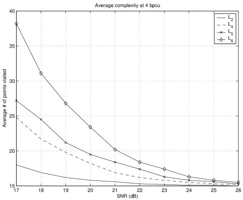
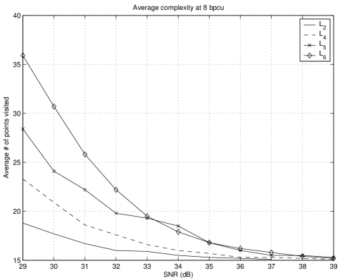
Figure 1: Average complexity of $4$ tx-antenna matrix lattices at rates (approximately) $R=4$ and $R=8$ bpcu.

As the Alamouti scheme [2] has a very efficient decoding algorithm available, and our quaternionic lattices have an Alamouti-like block structure, it is natural to ask whether any of the benefits of Alamouti decoding will survive for our lattices. We shall see that the block structure allows us to decode the two blocks independently from each other. The following simple observation is the underlying geometric reason for our ability to do this.

Lemma IV.1

Let $A$ and $B$ be two $n\times n$ matrices with the property that the matrices $A,B,A^{H},B^{H}$ commute. Let $\mathbf{h}\in\mathbb{C}^{2n}$ be any (row) vector and write

$$M(A,B)=\left(\begin{array}[]{cc}A&B\\ -B^{H}&A^{H}\\ \end{array}\right).$$

Then the vectors $\mathbf{h}M(A,0)$ and $\mathbf{h}M(0,B)$ are orthogonal to each other when we identify $\mathbb{C}^{2n}$ with $\mathbb{R}^{4n}$ and use the usual inner product of a vector space over the real numbers.

Proof:

With the identification $\mathbb{C}^{2n}=\mathbb{R}^{4n}$ the real inner product is the real part of the hermitian inner product $\langle\ ,\ \rangle$ of $\mathbb{C}^{2n}$. Write the vector $\mathbf{h}$ in the block form $\mathbf{h}=(h^{(1)},h^{(2)})$, where the blocks $h^{(j)},j=1,2$, are (row) vectors in $\mathbb{C}^{n}$. Then we can compute

$$\langle\mathbf{h}M(A,0),\mathbf{h}M(0,B)\rangle$$

$$= \langle\mathbf{h}M(A,0)M(0,B)^{H},\mathbf{h}\rangle$$

$$= \langle\mathbf{h}M(A,0)M(0,-B),\mathbf{h}\rangle$$

$$= \langle\mathbf{h}M(0,-AB),\mathbf{h}\rangle$$

$$= \langle h^{(2)}A^{H}B^{H},h^{(1)}\rangle-\langle h^{(1)}AB,h^{(2)}\rangle.$$

As $\langle\mathbf{u}M,\mathbf{v}\rangle=\langle\mathbf{v}M^{H},\mathbf{u}\rangle^{*}$ for all vectors $\mathbf{u},\mathbf{v}$ and matrices $M$, we see that the above hermitian inner product is pure imaginary. ∎

Corollary IV.2

Let $A$ and $B$ range over sets of $n\times n$-matrices. Let $\mathbf{h}$ and $\mathbf{r}$ be vectors in $\mathbb{C}^{2n}$. Then the Euclidean distance between $\mathbf{r}$ and $\mathbf{h}M(A,B)$ is minimized for the $A=A_{0}$ and $B=B_{0}$, when $A_{0}$ minimizes the Euclidean distance between $\mathbf{r}$ and $\mathbf{h}M(A,0)$ and $B_{0}$ minimizes the Euclidean distance between $\mathbf{r}$ and $\mathbf{h}M(0,B)$.

Proof:

Write $V_{A}$ (resp. $V_{B}$) for the real vector space spanned by the vectors $\mathbf{h}M(A,0)$ (resp. $\mathbf{h}M(0,B)$). These subspaces are orthogonal to each other in the sense of Lemma IV.1. Whence we can uniquely write $\mathbf{r}=r_{A}+r_{B}+r_{\perp}$, where $r_{A}\in V_{A},r_{B}\in V_{B}$ and $r_{\perp}$ is in the (real) orthogonal complement of the direct sum $V_{A}\oplus V_{B}$. A similar decomposition for the vector $\mathbf{h}M(A,B)$ is $\mathbf{h}M(A,B)=h_{A}+h_{B}$, where $h_{A}=\mathbf{h}M(A,0)\in V_{A}$ and $h_{B}=\mathbf{h}M(0,B)\in V_{B}$. By the Pythagorean theorem

$$|\mathbf{r}-\mathbf{h}M(A,B)|^{2}=|r_{A}-\mathbf{h}M(A,0)|^{2}+|r_{B}-\mathbf{h}M(0,B)|^{2}+|r_{\perp}|^{2}.$$

Furthermore, here

$$|r_{A}-\mathbf{h}M(A,0)|^{2}=|\mathbf{r}-\mathbf{h}M(A,0)|^{2}-|r_{B}|^{2}-|r_{\perp}|^{2},$$

so the quantities $|r_{A}-\mathbf{h}M(A,0)|^{2}$ and $|\mathbf{r}-\mathbf{h}M(A,0)|^{2}$ are minimized for the same choice of the matrix $A$. A similar argument applies to the $B$-components, so the claim follows. ∎

IV-B Complexity issues and collapsing lattices

The number of nodes in the search tree is used as a measure of complexity so that the implementation details or the physical environment do not affect it. We have analyzed many different kinds of situations concerning the change of complexity of the sphere decoder when moving in (1) from right to left.

In Fig. 1 we have plotted the average number of points visited by the algorithm in different cases at the rates approximately $4$ and $8$ bpcu. The SNR regions cover the block error rates between $\approx 10\%-0.01\%$. As can be seen, in the low SNR end, the difference in complexity between the different lattices is clear but evens out when the SNR increases. For the sublattices $L_{4},\ L_{5}$, and $L_{6}$ the algorithm visits $1.1-2.1$ times as many points as for the base lattice $L_{2}$. In the larger SNR end, the performance is fairly similar for all the lattices. E.g. at $4$ and $8$ bpcu, when all the lattices reach the bound of maximum 20 points visited, the block error rates of $L_{4},\ L_{5}$, and $L_{6}$ are still as big as $5\%,\ 2\%$, and $1\%$ respectively.

Definition IV.1

In a MISO setting we say that a matrix lattice $L$ of rank $m$ collapses at a channel realization $\mathbf{h}$, if the receiver’s version of the lattice $\mathbf{h}L$ spans a real vector space of dimension $<m$. We call the set of such channel realizations the critical set. We say that the sensitivity $s(L)$ (towards collapsing) of the lattice $L$ is $r$, if the critical set is a union of finitely many subspaces of real dimension $\leq r$.

So we e.g. immediately see that a lattice residing in an orthogonal design will have zero sensitivity. While we have no precise results the thinking underlying the concept can be motivated as follows. When the infinite lattice collapses into a lower dimensional space, its linear structure is severely mutilated. For example the minimum Euclidean distance drops to zero — for any $\epsilon>0$ there will be infinitely many other lattice points within a distance $<\epsilon$. Even when we restrict ourselves to a finite subset of the lattice, the coordinates of the nearby points may differ drastically. Thus even an ML-decoder will have problems, and an algorithm relying on the orderly linear structure of the lattice (like the sphere decoder) cannot work very efficiently. Similar problems are still there, when the actual channel realization $\mathbf{h}$ is close to a critical vector.

The sensitivity then enters the scene as a crude measure for the probability of this happening. It is easy to see that in a Rayleigh fading channel the probability of the channel vector $\mathbf{h}$ to be within $\epsilon$ of a critical vector behaves like ${\cal O}(\epsilon^{2n-s})$. Thus the lower the sensitivity, the lower the probability of the lattice becoming distorted by the channel.

We lead off by determining the sensitivity of the DAST-lattices.

Example IV.1

There exist 8-dimensional lattices [5] of $4\times 4$ matrices of the form

$$M_{DAST}=\left(\begin{array}[]{rrrr}x_{1}&x_{2}&x_{3}&x_{4}\\ x_{1}&-x_{2}&x_{3}&-x_{4}\\ x_{1}&x_{2}&-x_{3}&-x_{4}\\ x_{1}&-x_{2}&-x_{3}&x_{4}\\ \end{array}\right).$$

These matrices are simultaneously diagonalizable as they have common orthogonal eigenvectors $\mathbf{h}_{1}=(1,1,1,1)$, $\mathbf{h}_{2}=(1,-1,1,-1)$, $\mathbf{h}_{3}=(1,1,-1,-1)$ and $\mathbf{h}_{4}=(1,-1,-1,1)_{4}$. Write the channel vector in terms of this basis $\mathbf{h}=\sum_{j=1}^{4}a_{j}\mathbf{h}_{j}$. If any of the coefficients vanishes, say $a_{k}=0$, then the DAST-lattice collapses, because the receiver’s version of the lattice will belong to the complex span of the other three eigenvectors $\mathbf{h}_{j},j\neq k$. On the other hand, if all the coefficients $a_{j}\neq 0,j=1,2,3,4$, this channel vector will not be critical. One way of seeing this is that applying the linear mapping determined by $\mathbf{h}_{j}\mapsto(1/a_{j})\mathbf{h}_{j}$ to the receiver’s lattice then recovers the original full rank lattice of vectors $(x_{1},x_{2},x_{3},x_{4})$. Such a mapping obviously cannot affect the dimension of the space spanned by the vectors, so the lattice won’t collapse.

We have shown that the sensitivity of the DAST-lattice is six.

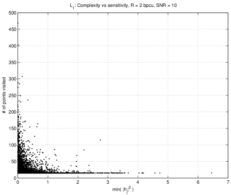
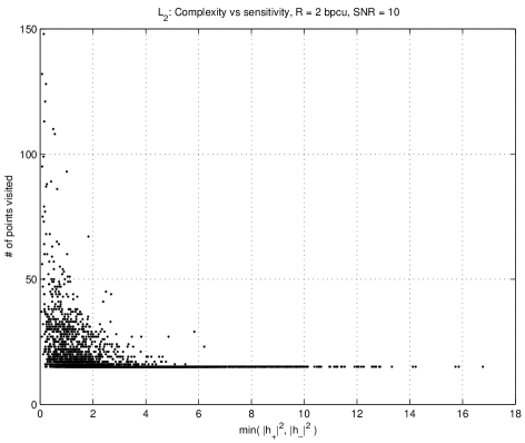
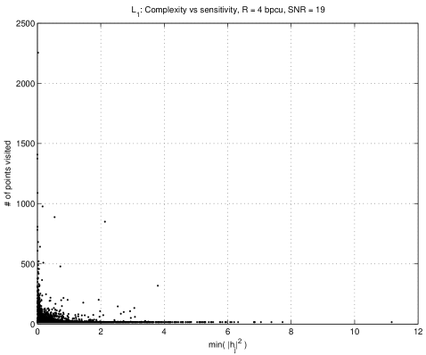
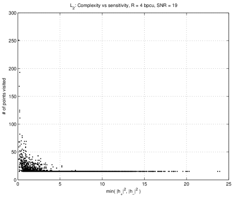
Figure 2: The impact of sensitivity on complexity, $L_{1}\ (\approx L_{DAST})$ vs $L_{2}$.

We proceed to determine the sensitivities of the lattices $L_{1}$ of Proposition II.2 and the ones within the nested sequence (1). Let us first consider $L_{1}$. Let

$$U=\left(\begin{array}[]{rrr}\mathbf{h}_{1}\\ \vdots\\ \mathbf{h}_{4}\\ \end{array}\right)$$

be the $4\times 4$ matrix with rows $\mathbf{h}_{1},\mathbf{h}_{2},\mathbf{h}_{3},\mathbf{h}_{4}$ of the form $(1,\zeta^{j},\zeta^{2j},\zeta^{3j})$ for $j=1,5,9,13$. Recall that earlier we have used $\{1,\zeta,\zeta^{2},\zeta^{3}\}$ as an integral basis, so the rows of $U$ are the images of this ordered basis under the action of the Galois group $G$ of the extension $\mathbb{Q}(\zeta)/\mathbb{Q}(i)$. Now it happens that the matrix $U$ is unitary (up to a constant factor) as $UU^{*}=4I_{4}$. Let $z=c_{1}+c_{2}\zeta+c_{3}\zeta^{2}+c_{4}\zeta^{3}$ be an arbitrary algebraic integer of $\mathbb{Q}(\zeta)$, and $M(z)=M_{L}(c_{1},c_{2},c_{3},c_{4})\in L_{1}$ be the corresponding matrix of Proposition II.2. According to the theory of algebraic numbers (and also trivially verified by hand) the rows of $U$ are (left) eigenvectors of $M(z)$, and

$$UM(z)U^{-1}=\left(\begin{array}[]{cccc}z&0&0&0\\ 0&\sigma_{2}(z)&0&0\\ 0&0&\sigma_{3}(z)&0\\ 0&0&0&\sigma_{4}(z)\end{array}\right)$$

is a diagonal matrix with entries gotten by applying the elements of the Galois group $G=\{\sigma_{1}=id,\sigma_{2},\sigma_{3},\sigma_{4}\}$ to the number $z$.

So all the matrices $M_{L}(c_{1},c_{2},c_{3},c_{4})$ are diagonalized by $U$. Therefore we might call the lattice $L_{1}$ ‘DAST-like’, as it shares this property with the lattices from [5].

Proposition IV.3

The lattice $L_{1}$ has sensitivity six.

Proof:

The situation is completely analogous to that of Example IV.1. The lattice $L_{1}$ will collapse, iff the channel realization belongs to any of the 4 complex vector spaces spanned by any three of the common eigenvectors. ∎

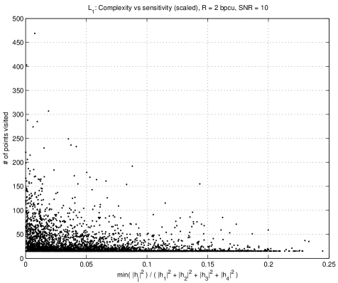
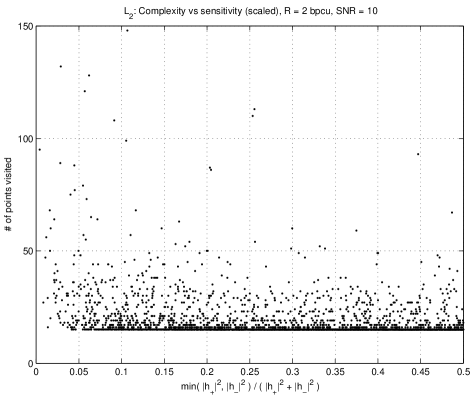
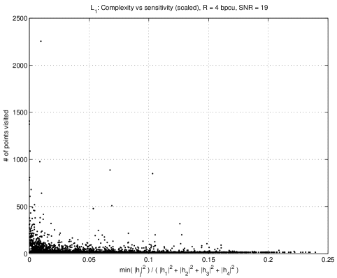
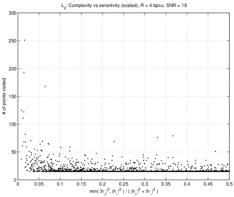
Figure 3: The scaled impact of sensitivity on complexity, $L_{1}\ (\approx L_{DAST})$ vs $L_{2}$.

In order to study the quaternionic lattices we first observe that the $2\times 2$-matrices $A$ and $B$ appearing as blocks of a matrix $M\in L_{2}$ all have $(1,\pm\xi)$ as their common (left) eigenvectors. The same holds for the adjoints $A^{*},B^{*}$ as they also appear as blocks of $M^{*}$ that also happens to belong to the lattice $L_{2}$. From the proof of Proposition II.4 we see that the matrix $MM^{*}$, $M=M(c_{1},c_{2},c_{3},c_{4})$, has eigenvalues $\alpha\pm|k|$ with respective (left) eigenvectors $(1,\pm\xi,0,0)$ and $(0,0,1,\pm\xi)$. Here $\alpha=\sum_{j=1}^{4}|c_{j}|^{2}$ and $k=-ic_{1}c_{2}^{*}+c_{2}c_{1}^{*}-ic_{3}c_{4}^{*}+c_{4}c_{3}^{*}$. We make this more precise before we determine the sensitivity of the quaternionic lattices.

There is a connection between our MISO-code and the multi-block codes introduced by Belfiore in [45] and Lu in [44] that can be best explained with the notation of the present section. Consider the unitary matrix with the above basis vectors as columns

$$U=\frac{1}{\sqrt{2}}\left(\begin{array}[]{cccc}1&1&0&0\\ \xi&-\xi&0&0\\ 0&0&1&1\\ 0&0&\xi&-\xi\end{array}\right).$$

If we conjugate the matrices of the algebra ${\bf H}$ by $U$ we get matrices of the form

$$\left(\begin{array}[]{cccc}x_{1}&-x_{2}^{*}&0&0\\ x_{2}&x_{1}^{*}&0&0\\ 0&0&\tau(x_{1})&-\tau(x_{2})\\ 0&0&\tau(x_{2})&\tau(x_{1})^{*}\end{array}\right),$$

where the elements $x_{1},x_{2}$ belong to the field $\mathbb{Q}(\xi)=\mathbb{Q}(i,\sqrt{2})$, and $\tau:\mathbb{Q}(\xi)\rightarrow\mathbb{Q}(\xi)$ is the automorphism determined by $\tau(i)=i$, $\tau(\sqrt{2})=-\sqrt{2}$. Thus we see that our MISO-code is unitarily equivalent to a multi-block code with a structure similar to [44] — only our center is smaller.

The upshot here, as well as in [45], [44], and in the icosian construction from [38] is that while the individual diagonal blocks may have arbitrarily small determinants, when we use them together with their algebraic conjugates, the diagonal blocks together conspire to give a non-vanishing determinant. This is because the algebraic conjugates of small numbers are necessarily just large enough to compensate as the algebraic norms are known to be integers.

Another benefit enjoyed by our matrix representation of the algebra ${\bf H}$ over the above multi-block representation is that the signal constellation is better behaved. Surely the simple QAM-constellation of our matrices is to be preferred over the linear combinations of two rotated QAM-symbols of the multi-block representation.

This feature clearly begs to be generalized to a MIMO-setting. One such construction is the previously mentioned icosian construction of Liu & Calderbank [38], where they managed to add a multiplexing gain of 2 to a similar multi-block representation of the icosians. It turned out that the question of how to best do this in the spirit of the present article is somewhat delicate. The resulting codes will necessarily be asymmetric MIMO-codes, and we refer the reader to [46].

We return to the sensitivity of the quaternionic lattices. The following result is now easy to verify

Proposition IV.4

Let $V_{+}$ (resp. $V_{-}$) be the complex subspace of $\mathbb{C}^{4}$ generated by the vectors $(1,\xi,0,0)$ and $(0,0,1,\xi)$ (resp. by $(1,-\xi,0,0)$ and $(0,0,1,-\xi)$). The subspaces $V_{+}$ and $V_{-}$ are orthogonal complements of each other in $\mathbb{C}^{4}$, so any channel vector can be uniquely written as

$$\mathbf{h}=\mathbf{h}_{+}+\mathbf{h}_{-},$$

where $\mathbf{h}_{\pm}\in V_{\pm}$ respectively. If $\mathbf{h}$ belongs to one of the subspaces $V_{+},V_{-}$, the lattice $\mathbf{h}L_{2}$ collapses. Otherwise the lattice $L_{2}$ does not collapse. In particular the sensitivity of the lattices $L_{2},L_{3},L_{4},L_{5},L_{6}$ is four. ∎

Our simulations, indeed, show that the complexity of a sphere decoder increases sharply, when we approach the critical set. A comparison between the lattices $L_{1}$ and $L_{2}$ does not show a dramatic difference between the average complexities of a sphere decoder, but the difference becomes very apparent, when studying the high-complexity tails of the complexity distribution.

In Fig. 2 we have plotted the complexity distribution of 5000 transmissions for different data rates. On the horizontal axis the quantity min$(\ |\mathbf{h}_{i}|^{2}\ )$ (resp. min$(\ |\mathbf{h}_{+}|^{2},|\mathbf{h}_{-}|^{2}\ )$) describes how close the lattice $L_{1}$ (resp. $L_{2}$) is to the situation where it would collapse. That is, how close to zero the minimum of the components $\mathbf{h}_{i}\in V_{i},\ i=1,2,3,4$, (resp. $\mathbf{h}_{\pm}\in V_{\pm}$) gets (cf. Remark IV.3 and Proposition IV.4). For both $L_{1}$ and $L_{2}$ the figure shows that the smaller the quantity, the higher the complexity. We can also conclude that the lattice $L_{1}$ nearly collapses a lot more often than the lattice $L_{2}$. In addition, the number of points visited by the sphere decoding algorithm is much higher for $L_{1}$ than for $L_{2}$. These are phenomena caused by the higher sensitivity of $L_{1}$. In Fig. 3 the scaled impact of sensitivity is depicted.

Note that as $L_{DAST}$ has the same sensitivity as $L_{1}$, we can equally well analyze the behavior of the DAST lattice on the basis of Fig. 2 and Fig. 3.

V Energy considerations and simulations

As a summary of Propositions II.2–II.6 we get the following.

Proposition V.1

(1) The lattice $L_{2}$ is isometric to the rectangular lattice $\mathbb{Z}^{8}$ and has a minimum determinant equal to $1$.

(2) The lattice $L_{4}$ isometric to $D_{8}$ is an index two sublattice of $L_{2}$ and has a minimum determinant equal to $4$.

(3) The lattice $L_{5}$ isometric to $D_{4}\bot D_{4}$ is an index four sublattice of $L_{2}$ and has a minimum determinant equal to $16$.

(4) The lattice $L_{6}$ isometric to $E_{8}$ is an index 16 sublattice of $L_{2}$ and has a minimum determinant equal to $64$. ∎

In order to compare these lattices we scale them to the same minimum determinant. When a real scaling factor $\rho$ is used the minimum determinant is multiplied by $\rho^{2}$. As all the lattices have rank 8, the fundamental volume is then multiplied by $\rho^{8}$. Let us choose the units so that the fundamental volume of $L_{2}$ is $m(L_{2})=1$. Then after scaling $m(L_{4})=1/2$, $m(L_{5})=1/4$, and $m(L_{6})=1/4$. As the density of a lattice is inversely proportional to the fundamental volume, we thus expect the codes constructed within e.g. the lattices $L_{4}$ and $L_{6}$ to outperform the codes of the same size within $L_{2}$.

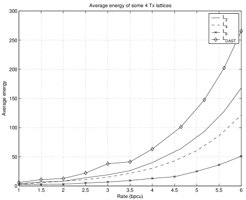
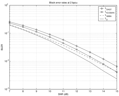
Figure 4: Average energy (left) and block error rates of $4$ Tx-antenna lattices at $2$ bpcu with one receiver (right).

The exact average transmission power data in Fig. 4 is computed as follows. Given the size $K$ of the code we choose a random set of $K$ shortest vectors from each lattice. The average energy of the code

$$E_{av}=\frac{\sum_{x\in\mathcal{C}}\|x\|^{2}}{K}$$

is then computed with the aid of theta functions [31]. All the lattices were normalized to have minimum determinant equal to 1. When using the matrices $M(c_{1},c_{2},c_{3},c_{4})$ of Proposition II.1, in some cases we are better off selecting the input vectors $(c_{1},c_{2},c_{3},c_{4})$ from the coset $\frac{1}{2}(1+i,1+i,1+i,1+i)+{\cal G}^{4}$ instead of letting them range over ${\cal G}^{4}$. Obviously such a translation does not change the minimum determinant of the code, but it sometimes results in significant energy savings. E.g. to get a code of size 256 it is clearly desirable to let the coefficients $c_{1},c_{2},c_{3},c_{4}$ range over the QPSK-alphabet.

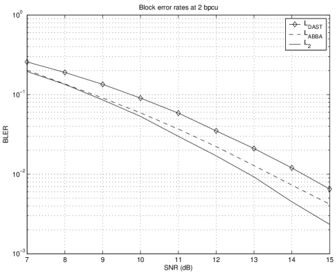
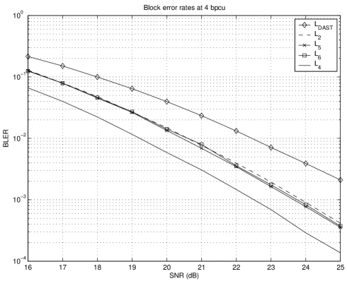
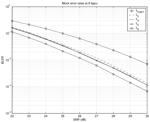
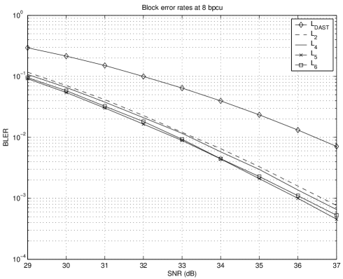
Figure 5: Block error rates of $4$ tx-antenna lattices at approximately $2.0$, $4.0$, $6.0$, and $8.0$ bpcu with one receiver.

Fig. 5 shows the block error rates of the various competing lattice codes at the rates approximately 2, 4, 6, and 8 bpcu, i.e. all the codes contain roughly $2^{8},2^{16},2^{24}$ or $2^{32}$ matrices respectively. For the lattices $L_{1}$, $L_{2}$, $L_{DAST}$, and $L_{ABBA}$ [20] this simply amounted to letting the coefficients $c_{1},c_{2},c_{3},c_{4}$ take all the values in a QPSK-alphabet. Therefore, it would have been easy to obtain bit error rates as well. For the lattices $L_{4}$, $L_{5}$, $L_{6}$ the rate is not exact, see (10) below and the preceding explanation. Of course also the exact rate equal to a power of two could be achieved by just choosing a more or less random set of shortest lattice vectors. As there is no natural way to assign bit patterns to vectors of $D_{8}$, $D_{4}\bot D_{4}$ or $E_{8}$, we chose to show the block error rates instead of the bit error rates.

The simulations were set up, here, so that the 95 per cent reliability range amounts to a relative error of about 3 per cent at the low SNR end and to about 10 per cent at the high SNR end (or to about 4000 and 400 error events respectively). One receiver was used for all the lattices.

When moving left in (1) the minimum determinant increaces while the BLER decreases at the same time. However, the other side of the coin is that improvements in the BLER performance cause a slightly more complex decoding process by increasing the number of points visited in the search tree. Still after this increasement, even the lattice $L_{6}$ admits a fairly low average complexity as compared to the lattices $L_{1}$ and $L_{DAST}$ due to its lower sensitivity. In part of the pictures in Fig. 5, the order of the curves seems not to respect the above mentioned order, but this only happens because the rates are not exactly the same for all the lattices. E.g. at the rate $\approx 4$ bpcu, the exact rates for $L_{2},L_{4},L_{5},$ and $L_{6}$ are $4,3.75,4.14,$ and $4.17$ bpcu respectively. Consequently, the lattice $L_{4}$ seems to perform better than what it actually does. Let us shortly explain how these rates follow: when picking the elements $x_{1},...,x_{8}$ from the set $\mathbb{Z}_{Q}$ (cf. Section IV (5) and the discussion after Algorithm II), the size of the code within the lattice $L_{i},\ i=2,4,5,6$, will be $\frac{Q^{8}}{[L_{2}:L_{i}]}=2^{\textrm{log}\frac{Q^{8}}{[L_{2}:L_{i}]}}$, where $[L_{2}:L_{i}]$ is the index of the sublattice $L_{i}$ inside $L_{2}$ (cf. Proposition V.1). Hence, the data rate in bits per channel use can be computed as

$$R=\frac{\textrm{log}\frac{Q^{8}}{[L_{2}:L_{i}]}}{4}.$$ (10)

Now, for instance, to get as close to the rate $R=4$ bpcu as possible, we have to choose $Q=4,Q=4,Q=5,$ and $Q=6$ for the lattices $L_{2},L_{4},L_{5},$ and $L_{6}$ respectively. By substituting $Q$ and the sublattice index in question to (10) we obtain the above rates.

Simulations at the rate $6$ bpcu with one receiver show that the lattice $L_{6}$ wins by approximately $1$ dB over the lattice $L_{2}$ and by at least $2.5$ dB over $L_{DAST}$. At the rate $2$ bpcu, the rotated ABBA lattice $L_{ABBA}$ is already beaten by the $L_{2}$ lattice by a fraction of a dB. The difference between $L_{2}$ and $L_{DAST}$ is even clearer: $L_{2}$ gains $1-2$ dB over $L_{DAST}$, depending on the SNR. At all data rates the lattice $L_{6}$ outperforms all the other lattices.

Prompted by the question of one of the reviewers, we make the following remark in case that the reader is familiar with the Icosian code [38] and ponders over whether and how it relates to the codes presented in this paper.

Remark V.1

The Icosian lattice $L_{ICOSIAN}$ presented in [38] takes use of the Icosian ring (cf. Remark III.6) and has a similar looking structure to the Golden code [11], where the matrix elements are replaced with Icosian Alamouti blocks

$$A=A(a_{1},a_{2},a_{3},a_{4})=\begin{pmatrix}a_{1}+a_{2}i&-a_{3}+a_{4}i\\ a_{3}+a_{4}i&a_{1}-a_{2}i\end{pmatrix}$$

and $B=B(b_{1},b_{2},b_{3},b_{4})$ respectively:

$$L_{ICOSIAN}=\left\{\begin{pmatrix}A&K\overline{B}\\ B&\overline{A}\end{pmatrix}\ \Big{|}\ a_{i},b_{i}\in\mathbb{Z}[(1+\sqrt{5})/2]\ \forall i\right\},$$

where $\overline{A}$ denotes the algebraic conjugate of $A$ with respect to the mapping $\sqrt{5}\mapsto-\sqrt{5}$ and

$$K=\begin{pmatrix}i&0\\ 0&-i\end{pmatrix}.$$

A code within this lattice is called Icosian code. Note that Jafarkhani’s quasi-orthogonal code [30] in the simulations of [38] is exactly our base lattice $L_{2}$.

First of all, note that the Icosian code has code rate two, as the lattice is 16-dimensional over the reals. Hence, in order to enable efficient linear decoding, at least two antennas are required at the receiving end. Taking this into consideration, there is no good way to make fair comparison between the Icosian lattice and the 8-dimensional lattices proposed in this paper. If the application at hand allows us to use one receiving antenna only, we either have to puncture $L_{ICOSIAN}$ (e.g. by setting $B=0$) which will cause it to lose its benefits, or, we need to perform complex decoding process (e.g. a sphere decoder cannot be used).

However, if we still want to compare these codes with two receivers, our codes will of course lose due to the lower code rate as they are designed for MISO use only. Similar comparison could be done e.g. with the $4\times 4$ Perfect code [11] and the Icosian code resulting to the loss of the Icosian code due to its lower rate (two vs. four). When using one receiver for the Icosian code by punctring the block $B$, it will lose to $L_{2}$ by 0.5-1 dB at 2 bpcu depending on the SNR as depicted in Figure 4. But, as noted above, in this way $L_{ICOSIAN}$ will of course lose its benefits (as we are not really using the whole Icosian ring) so this is not a comparison on which we should put too much value.

To conclude, the codes in this paper and the Icosian code are targeted into different types of applications: the first ones are aimed for systems with one receiving antenna, whereas the Icosian code naturally fits into systems with two receiving antennas.

VI Diversity-multiplexing tradeoff analysis

This section contains the DMT analysis of the MISO codes constructed in this paper. We denote by $n_{t}$ (resp. $n_{r}$) the number of transmitting (resp. receiving) antennas. For the rest of the notation, see [21].

Let us first consider the number field construction. Denote (cf. Proposition II.2)

$$L_{1}\ =\ \left\{\left(\begin{array}[]{cccc}c_{1}&ic_{4}&ic_{3}&ic_{2}\\ c_{2}&c_{1}&ic_{4}&ic_{3}\\ c_{3}&c_{2}&c_{1}&ic_{4}\\ c_{4}&c_{3}&c_{2}&c_{1}\end{array}\right),c_{i}\in{\cal A}\right\},$$

where ${\cal A}\subset\mathbb{Z}[i]$ is some constellation set. This code is for the MISO system with $n_{t}=4$ transmit and $n_{r}=1$ receive antennas. Given the transmit code matrix $X\in L_{1}$, the received signal vector is

$$\underline{y}^{T}\ =\ \theta\underline{h}^{T}X+\underline{n}^{T},$$

where $\underline{h}\sim\mathbb{C}{\cal N}(\underline{0},I_{4})$.

Let $r$ be the desired multiplexing gain; then we need

$$\left|L_{1}\right|\ \doteq\ \mbox{{SNR}}^{4r}\ \doteq\ \left|{\cal A}\right|^{4}$$

and the above in turn gives

$$\left|{\cal A}\right|\ \doteq\ \mbox{{SNR}}^{r}.$$ (11)

Hence we see for every $c_{i}\in{\cal A}$

$$\left\|c_{i}\right\|^{2}\ \dot{\leq}\ \mbox{{SNR}}^{r}$$ (12)

and

$$\theta^{2}\ \doteq\ \mbox{{SNR}}^{1-r}.$$ (13)

Let $\lambda:=\left\|\underline{h}\right\|_{F}^{2}=\mbox{{SNR}}^{-\alpha}$ and let $\delta_{1}\geq\cdots\geq\delta_{4}$ be the ordered eigenvalues of $XX^{\dagger}$; then the random Euclidean distance $d_{E}$ is lower bounded by

$$d_{E}^{2}\geq\theta^{2}\lambda\delta_{4}\doteq\frac{\theta^{2}\lambda}{\prod_{i=1}^{3}\delta_{i}}\ \dot{\geq}\ \mbox{{SNR}}^{E_{L_{1}}}$$ (14)

where

$${E_{L_{1}}}\ =\ 1-r-\alpha-3r=1-4r-\alpha.$$ (15)

Now the DMT of this code is given by

$$d_{L_{1}}(r)\ \geq\ \inf_{{E_{L_{1}}}<0}4\alpha\ =\ 4(1-4r),\ \ \text{ for $0\leq r\leq\frac{1}{4}$,}$$ (16)

while the optimal tradeoff in this channel is actually

$$d^{*}(r)\ =\ 4(1-r)\ \ \text{ for $0\leq r\leq 1$.}$$ (17)

The quaternionic construction is

$$L_{2}\ =\ \left\{\left(\begin{array}[]{cccc}c_{1}&ic_{2}&-c_{3}^{*}&-c_{4}^{*}\\ c_{2}&c_{1}&ic_{4}^{*}&-c_{3}^{*}\\ c_{3}&ic_{4}&c_{1}^{*}&c_{2}^{*}\\ c_{4}&c_{3}&-ic_{2}^{*}&c_{1}^{*}\end{array}\right),c_{i}\in{\cal A}\right\}.$$

First of all, as pointed out in the proof of Proposition 2.4, the matrix $M\in L_{2}$ is of the following form:

$$M\ =\ \left(\begin{array}[]{cc}A&-B^{H}\\ B&A^{H}\end{array}\right)$$

and

$$MM^{H}\ = \ \left(\begin{array}[]{cc}AA^{H}+B^{H}B&{\bf 0}\\ {\bf 0}&A^{H}A+BB^{H}\end{array}\right)$$

$$= \left(\begin{array}[]{cc}AA^{H}+BB^{H}&{\bf 0}\\ {\bf 0}&AA^{H}+BB^{H}\end{array}\right)$$

since $AB=BA$. Thus the ordered eigenvalues of $MM^{H}$ satisfy $\delta_{1}=\delta_{2}\geq\delta_{3}=\delta_{4}$ and in particular, $\delta_{1}\geq\delta_{3}$ are the ordered eigenvalues of $AA^{H}+BB^{H}$. Secondly, note that $MM^{H}$ satisfies the non-vanishing determinant property, and so does the matrix $AA^{H}+BB^{H}$. Now the bound for the random Euclidean distance is

$$d_{E}^{2}\ \geq\ \theta^{2}\lambda\delta_{4}\ \doteq\ \frac{\theta^{2}\lambda}{\delta_{3}}\ \dot{\geq}\mbox{{SNR}}^{E_{L_{2}}},$$ (20)

where

$$E_{L_{2}}\ =\ 1-r-\alpha-r=1-2r-\alpha.$$ (21)

Now the DMT of this code is given by

$$d_{L_{2}}(r)\ \geq\ \inf_{{E_{L_{2}}}<0}4\alpha\ =\ 4(1-2r),\ \ \text{ for $0\leq r\leq\frac{1}{2}$.}$$ (22)

The same of course also holds for codes within the sublattices $L_{4},L_{5},L_{6}\subseteq L_{2}$.

Remark VI.1

While our codes are not DMT optimal, it has to be noticed that without using a full-rate code the DMT cannot be achieved. Hence, if one wishes to enable efficient decoding process with one receiving antenna only (see the remark below), sacrifices in terms of the DMT have to be made. However, our quaternionic lattices $L_{2},L_{4},L_{5},L_{6}$ admit higher DMT as e.g. the DAST lattice, as the DMT of the DAST lattice coincides with that of $L_{1}$.

Remark VI.2

One might ponder why not use e.g. the full-rate CDA based codes (cf. [6], [11]) as they are DMT optimal provided that they have non-vanishing determinant. The answer to this is in principle the same as the one provided in Remark V.1. We could naturally do this, but considering that we only want to use one receiving antenna it should be clear that a full-rate code cannot be efficiently used. Indeed, using a full-rate code would destroy the lattice structure and cause exponential complexity at the receiver. To enable efficient decoding with one receiver we have to limit ourselves to rate-one codes, which exactly we have done in this paper. We want the reader to note that full-rate codes (e.g. the perfect codes [11]) are optimally suited for systems with $n_{t}=n_{r}>1$, hence inapplicable to the purposes of this paper where we have $n_{t}=4$ and $n_{r}=1$.

VII Conclusions and suggestions for further research

In this paper, we have presented new constructions of rate-one, full-diversity, and energy efficient $4\times 4$ space-time codes with non-vanishing determinant by using the theory of rings of algebraic integers and their counterparts within the division rings of Lipschitz’ and Hurwitz’ integral quaternions. A comfortable, purely number theoretic way to improve space-time lattice constellations was introduced. The use of ideals provided us with denser lattices and an easy way to present the exact proofs for the minimum determinants. The constructions can be extended also to a larger number of transmit antennas, and they nicely fit with the popular Q²-QAM and QPSK modulation alphabets. The idea of finding denser sublattices within a given division algebra was also generalized to a MIMO case with arbitrary number of Tx antennas by using the theory of cyclic division algebras and, as a novel method, their maximal orders. This is encouraging as the CDA based square ST constructions with NVD are known to achieve the DMT. We have also shown that the explicit constructions in this paper all have a simple decoding method based on sphere decoding. Related to the decoding complexity, the notion of sensitivity was introduced for the first time in this paper. The experimental results have given evidence about the relevance of this new notion.

Comparisons with the four antenna DAST block code have shown that our codes provide lower energy and block error rates due to their good minimum determinant, i.e. high density and lower sensitivity. At the moment, we are searching for well-performing MIMO codes arising from the theory of crossed product algebras and maximal orders of cyclic division algebras. We have noticed that also the discriminant of a maximal order plays an important role in code design. It is desirable to choose cyclic division algebras for which the discriminant of a maximal order is as small as possible [33]. By now, we are able to construct an explicit cyclic division algebra of an arbitrary index over $\mathbb{Q}(i)$ (or $\mathbb{Q}(\omega)$) that has a maximal order with minimal discriminant. Despite the fact that we have not yet fully analyzed the practical performance of codes arising from these constructions, the preliminary results have been very promising. Further details on this and on the algorithmic properties of maximal orders (see also [47]-[49]) will be given in a forthcoming paper [33].

VIII Acknowledgments

The authors are grateful to graduate student Miia Mäki for partly implementing the sphere decoder that was used for the simulations. A thank-you is also due to anonymous reviewers for their insightful comments that greatly improved the quality of this paper.

C. Hollanti was supported in part by the Nokia Foundation, the Foundation of Technical Development, and the Foundation of the Rolf Nevanlinna Institute, Finland.

References

- [1] J.-C. Guey, M. P. Fitz, M. R. Bell, and W. Y. Kuo, “Signal design for transmitter diversity wireless communication systems over Rayleigh fading channels”, in Proc. IEEE Vehicular Technology Conf., 1996, pp. 136–140. Also in IEEE Trans. Commun., vol. 47, pp. 527–537, April 1999.
- [2] S. M. Alamouti, “A Simple Transmit Diversity Technique for Wireless Communication”, IEEE J. on Select. Areas in Commun., vol. 16, pp. 1451–1458, October 1998.
- [3] J. Hiltunen, C. Hollanti, and J. Lahtonen, “Four Antenna Space-Time Lattice Constellations from Division Algebras”, in Proc. IEEE ISIT 2004, p. 338., Chicago, June 27 - July 2, 2004.
- [4] J. Hiltunen, C. Hollanti, and J. Lahtonen, “Dense Full-Diversity Matrix Lattices for Four Antenna MISO Channel”, in Proc. IEEE ISIT 2005, pp. 1290–1294, Adelaide, September 4 - 9, 2005.
- [5] M. O. Damen, K. Abed-Meraim, and J.-C. Belfiore, “Diagonal Algebraic Space-Time Block Codes”, IEEE Trans. Inf. Theory, vol. 48, pp. 628–636, March 2002.
- [6] B. A. Sethuraman, B. S. Rajan, and V. Shashidhar, “Full-Diversity, High-Rate Space-Time Block Codes From Division Algebras”, IEEE Trans. Inf. Theory, vol. 49, pp. 2596–2616, October 2003.
- [7] J.-C. Belfiore and G. Rekaya, “Quaternionic Lattices for Space-Time Coding”, in Proc. ITW 2003, Paris, France, March 31 - April 4, 2003.
- [8] J.-C. Belfiore, G. Rekaya, and E. Viterbo, “The Golden Code: A 2x2 Full-Rate Space-Time Code with Non-Vanishing Determinants”, in Proc. IEEE ISIT 2004, p. 308, Chicago, June 27 - July 2, 2004.
- [9] H. Yao and G. W. Wornell, “Achieving the Full MIMO Diversity-Multiplexing Frontier with Rotation-Based Space-Time Codes”, in Proc. Allerton Conf. Commun., contr., and Computing, Oct. 2003.
- [10] J.-C. Belfiore, G. Rekaya, and E. Viterbo, “Algebraic 3x3, 4x4 and 6x6 Space-Time Codes with Non-Vanishing Determinants”, in Proc. IEEE ISITA 2004, Parma, Italy, October 10 - 13, 2004.
- [11] J.-C. Belfiore, F. Oggier, G. Rekaya, and E. Viterbo, “Perfect Space-Time Block Codes”, IEEE Trans. Inf. Theory, vol. 52, pp. 3885–3902, September 2006.
- [12] Kiran. T and B. S. Rajan, “STBC-Schemes with Non-Vanishing Determinant For Certain Number of Transmit Antennas”, IEEE Trans. Inf. Theory, vol. 51, pp. 2984–2992, August 2005.
- [13] V. Shashidhar, B. S. Rajan, and B. A. Sethuraman “STBCs using capacity achieving designs from crossed-product division algebras”, in Proc. IEEE ICC 2004, pp. 827–831, Paris, France, 20-24 June 2004.
- [14] V. Shashidhar, B. S. Rajan, and B. A. Sethuraman, “Information-Lossless STBCs from Crossed-Product Algebras”, IEEE Trans. Inf. Theory, vol. 52, pp. 3913–3935, September 2006.
- [15] P. Elia, K. R. Kumar, P. V. Kumar, H.-F. Lu, and S. A. Pawar, “Explicit Space-Time Codes Achieving the Diversity-Multiplexing Gain Tradeoff”, IEEE Trans. Inf. Theory, vol. 52, pp. 3869–3884, September 2006.
- [16] G. Wang and X.-G. Xia, “On Optimal Multi-Layer Cyclotomic Space-Time Code Designs”, IEEE Trans. Inf. Theory, vol. 51, pp. 1102–1135, March 2005.
- [17] M. O. Damen, H. E. Gamal, and N. C. Beaulieu, “Linear Threaded Algebraic Space-Time Constellations”, IEEE Trans. Inf. Theory, vol. 49, pp. 2372–2388, October 2003.
- [18] M. O. Damen and H. E. Gamal, “Universal Space-Time Coding”, IEEE Trans. Inf. Theory, vol. 49, pp. 1097–1119, May 2003.
- [19] P. Dayal and K. Varanasi, “Algebraic Space-Time Codes with Full Diversity and Low Peak-To-Mean Power Ratio”, in Proc. Commun. Th. Symp., IEEE GLOBECOM, San Francisco, CA, Dec. 2003.
- [20] O. Tirkkonen, A. Boariu, and A. Hottinen, “Minimal Non-Orthogonality Rate 1 Space-Time Block Code for 3+ TX Antennas”, in Proc. IEEE ISSSTA, vol. 2, pp. 429–432, September 2000.
- [21] L. Zheng and D. Tse, “Diversity and Multiplexing: A Fundamental Tradeoff in Multiple-Antenna Channels”, IEEE Trans. Inf. Theory, vol. 49, pp. 1073–1096, May 2003.
- [22] V. Tarokh, N. Seshadri, and A.R. Calderbank, “Space-Time Codes for High Data Rate Wireless Communications: Performance Criterion and Code Construction”, IEEE Transactions on Information Theory, vol. 44, pp. 744–765, March 1998.
- [23] I. Stewart and D. Tall, Algebraic Number Theory, Chapman and Hall, London 1979.
- [24] V. Tarokh, H. Jafarkhani, and A. R. Calderbank, “Space-Time Block Codes from Orthogonal Designs”, IEEE Transactions on Information Theory, vol. 45, pp. 1456–1467, July 1999.
- [25] O. Tirkkonen, “Optimizing Space-Time Block Codes by Constellation Rotations”, in Proceedings Finnish Wireless Communications Workshop FWCW’01, pp. 59–60, October 2001.
- [26] A. Hottinen and O. Tirkkonen, “Square-Matrix Embeddable Space-Time Block Codes for Complex Signal Constellations”, IEEE Trans. Inf. Theory, vol. 48 (2), pp. 384–395, February 2002.
- [27] J. Boutros, E. Viterbo, C. Rastello, and J.-C. Belfiore, “Good Lattice Constellations for Both Rayleigh Fading and Gaussian Channels”, IEEE Trans. Inf. Theory, vol. 42, pp. 502–518, March 1996.
- [28] B. Hassibi, B. M. Hochwald, A. Shokrollahi, and W. Sweldens, “Representation Theory for High-Rate Multiple-Antenna Code Design”, IEEE Trans. Inf. Theory, vol. 47, pp. 2335–2364, September 2001.
- [29] F. E. Oggier and E. Viterbo, “Algebraic number theory and code design for Rayleigh fading channels”, Foundations and Trends in Communications and Information Theory, December 2004.
- [30] H. Jafarkhani, “A Quasi-Orthogonal Space-Time Block Code”, IEEE WCNC, vol. 1, pp. 42–45, September 2000.
- [31] J. H. Conway and N. J. A. Sloane, Sphere Packings, Lattices and Groups, Grundlehren der Mathematischen Wissenschaften #290, Springer-Verlag, New York 1988.
- [32] D. Allcock, “New Complex- and Quaternion-Hyperbolic Reflection Groups”, Duke Mathematical Journal, vol. 103, pp. 303–333, June 2000.
- [33] C. Hollanti, J. Lahtonen, K. Ranto, and R. Vehkalahti, "Optimal Matrix Lattices for MIMO Codes from Division Algebras", in Proc. IEEE ISIT 2006, pp. 783–787, Seattle, July 9 - 14, 2006. Full paper submitted to IEEE Trans. Inf. Theory, Dec. 2006. Available at http://arxiv.org/abs/cs.IT/0703052.
- [34] N. Jacobson, Basic Algebra II, W. H. Freeman and Company, San Francisco 1980.
- [35] A. A. Albert, Structure of Algebras, American Mathematical Society, New York City 1939.
- [36] I. Reiner, Maximal Orders, Academic Press, London 1975.
- [37] C. Hollanti and J. Lahtonen, “A New Tool: Constructing STBCs from Maximal Orders in Central Simple Algebras”, in Proc. IEEE ITW 2006, pp. 322–326, Punta del Este, Uruguay, March 13-17, 2006.
- [38] J. Liu and A. R. Calderbank, “The Icosian Code and the Lattice: A New Space-Time Code with Nonvanishing Determinant”, in Proc. IEEE ISIT 2006, Seattle, July 9 - 14, 2006.
- [39] M. Pohst, “On the Computation of Lattice Vectors of Minimal Length, Successive Minima and Reduced Basis with Applications”, ACM SIGSAM, vol. 15, pp. 37–44, 1981.
- [40] E. Viterbo and J. Boutros, “A Universal Lattice Code Decoder for Fading Channel”, IEEE Transactions on Information Theory, vol. 45, pp. 1639–1642, July 1999.
- [41] E. Agrell, T. Eriksson, A. Vardy, and K. Zeger, “Closest Point Search in Lattices”, IEEE Transactions on Information Theory, vol. 48, pp. 2201–2214, August 2002.
- [42] M. O. Damen, A. Chkeif, and J.-C. Belfiore, “Lattice Codes Decoder for Space-Time Codes”, IEEE Commun. Lett., vol. 4, pp. 161–163, May 2000.
- [43] M. O. Damen, H. El Gamal, and G. Caire, “On Maximum-Likelihood Detection and the Search for the Closest Lattice Point”, IEEE Transactions on Information Theory, vol. 49, pp. 2389–2402, October 2003.
- [44] H.-f. (F.) Lu, “Explicit Constructions of Multi-Block Space-Time Codes that Achieve the Diversity-Multiplexing Tradeoff”, in Proc. IEEE ISIT 2006, pp. 1149–1153, Seattle, 2006.
- [45] S. Yang and J.-C. Belfiore, “Optimal Space-Time Codes for the MIMO Amplify-and-Forward Cooperative Channel”, IEEE Trans. Inf. Theory, vol. 53, pp. 647–663, Feb. 2007.
- [46] C. Hollanti and H.-f. (F.) Lu, “Normalized Minimum Determinant Calculation for Multi-Block and Asymmetric Space-Time Codes”, Applied Algebra, Algebraic Algorithms and Error Correcting Codes, pp. 227–237, Springer-Verlag LNCS 4851, Berlin 2007.
- [47] L. Rónyai, “Algorithmic Properties of Maximal Orders in Simple Algebras Over Q”, Computational Complexity 2, pp. 225–243, 1992.
- [48] G. Ivanyos and L. Rónyai, “On the complexity of finding maximal orders in algebras over Q”, Computational Complexity 3, pp. 245–261, 1993.
- [49] Web page: http://magma.maths.usyd.edu.au/magma/htmlhelp/text835.htm#8121.