Abstract

Since quarks are regarded as the most fundamental particles which constitute hadrons that we observe in the real world, there are many theories about how many of them are needed and what quantum numbers they carry. Another important question is what keeps them inside the hadron, which is known to have space-time extension. Since they are relativistic objects, how would the hadron appear to observers in different Lorentz frames? The hadron moving with speed close to that of light appears as a collection of Feynman’s partons. In other words, the same object looks differently to observers in two different frames, as Einstein’s energy-momentum relation takes different forms for those observers. In order to explain this, it is necessary to construct a quantum bound-state picture valid in all Lorentz frames. It is noted that Paul A. M. Dirac studied this problem of constructing relativistic quantum mechanics beginning in 1927. It is noted further that he published major papers in this field in 1945, 1949, 1953, and in 1963. By combining these works by Dirac, it is possible to construct a Lorentz-covariant theory which can explain hadronic phenomena in the static and high-speed limits, as well as in between. It is shown also that this Lorentz-covariant bound-state picture can explain what we observe in high-energy laboratories, including the parton distribution function and the behavior of the proton form factor.

1 Introduction

The hydrogen atom played the pivotal role in the development of quantum mechanics. Its discrete energy levels led to the concept of a localization condition for the probability distribution, and thus to the bound-state picture of quantum mechanics. Likewise, the quark model is still playing the central role in high-energy physics [1]. In this model, hadrons are bound states of more fundamental particles called“quarks” with their own internal quantum numbers, such as isospins, unitary spins, and then flavors.

Thus, the symmetry of combining these quantum numbers has been and still is an important branch of physics. Unlike the proton and electron in the hydrogen atom, quarks have never been observed as free particles. They are always confined inside the hadron. Thus the only way of determining their properties is through observing the symmetry properties of hadrons.

Then there comes the question of the binding forces between them, and the dynamics governing those forces. If the hadrons are assumed to be quantum bound states, there are localized probability distributions whose boundary conditions generate discrete mass spectra. This aspect of quantum mechanics is well known. On the other hand, it is not yet completely clear how the localized probability distribution would look to observers in different Lorentz frames. Protons coming from high-energy accelerators are quantum bound states seen in a Lorentz frame moving very fast with respect to their rest frame. This is the question on which we would like to concentrate in this review paper.

There are then three steps. First, we have to assemble the physical principles needed to construct this scheme. We shall need space-time transformation laws of special relativity and uncertainty principles of quantum mechanics applicable to position and momentum variables. Since we are interested in constructing a Lorentz-covariant theory, we need the time-energy uncertainty relation. However, this time-energy relation does not allow excited states, and has to be treated differently. This is the first hurdle we have to overcome.

The second step is to construct a mathematical formalism which will accommodate all the physical conditions presented in the first step. As always, harmonic oscillators serve as test models for all new theories. We shall construct a formalism based on harmonic oscillators, whose wave functions satisfy Lorentz-covariant boundary conditions, orthogonality conditions, the difference between position-momentum and time-energy uncertainty relations. This covariant oscillator formalism will satisfy all physical laws of quantum mechanics and special relativity.

The third step is to see whether the theory tells the story of the real world. For this purpose, we discuss in detail the proton form factors and Feynman’s parton picture [2, 3]. Indeed, it has been the most outstanding issue in high energy physics whether the quark model and parton model are two different limiting cases of one Lorentz-covariant entity. We examine this issue in detail.

This review paper is largely based on the papers published by the present authors. But we are not the first ones to approach the difficult problem of constructing a Lorentz-covariant picture of quantum bound states. Indeed, this problem was recognized earlier by Dirac, Wigner, and Feynman. We shall present a review of their valiant efforts in this direction. These great physicists constructed big lakes. We are connecting these lakes to construct a canal leading to an understanding of relativistic bound states applicable to the quark model and the parton model.

Einstein was against the Copenhagen interpretation of quantum mechanics. Why was he so against it? The present form of quantum mechanics is regarded as unsatisfactory because of its probabilistic interpretation. At the same time, it is unsatisfactory because it does not appear to be Lorentz-covariant. We still do not know how the hydrogen atom appears to a moving observer.

While relativity was Einstein’s main domain of interest, why did he not complain about the lack of Lorentz covariance? It is possible that Einstein was too modest to mention relativity, and instead concentrated his complaint against its probabilistic interpretation. It is also possible that Einstein did not want to send his most valuable physics asset to a battle ground. We cannot find a definite answer to this question, but it is gratifying to note that the present authors are not the first ones to question whether the Copenhagen school of thought is consistent with the concept of relativity [4].

Paul A. M. Dirac was never completely happy with the Copenhagen interpretation of quantum mechanics, but he thought it was a necessary temporary step. In that case, he thought we should examine whether quantum mechanics is consistent with special relativity.

As for combining quantum mechanics with special relativity, there was a giant step forward with the construction of the present form of quantum field theory. It leads to a Lorentz covariant S-matrix which enables us to calculate scattering amplitudes using Feynman diagrams. However, we cannot solve bound-state problems or localized probability distributions using Feynman diagrams [5].

Dirac was never happy with the present form of field theory [6], particularly with infinite quantities in its renormalization processes. Furthermore, field theory never addresses the issue of localized probability. Indeed, Dirac concentrated his efforts on determining whether localized probability distribution is consistent with Lorentz covariance.

In 1927 [7], Dirac noted that there is a time-energy uncertainty relation without time-like excitations. He pointed out that this space-time asymmetry causes a difficulty in combining quantum mechanics with special relativity.

In 1945 [8], Dirac constructed four-dimensional harmonic oscillator wave functions including the time variable. His oscillator wave functions took a normalizable Gaussian form, but he did not attempt to give a physical interpretation to this mathematical device.

In 1949 [9], Dirac emphasized that the task of building a relativistic quantum mechanics is equivalent to constructing a representation of the Poincaré group. He then pointed out difficulties in constructing such a representation. He also introduced the light-cone coordinate system.

In 1963 [10], Dirac used two coupled oscillators to construct a representation of the $O(3,2)$ deSitter group which later became the basic mathematics for two-photon coherent states known as squeezed states of light [11].

In this paper, we combine all of these works by Dirac to make the present form of uncertainty relations consistent with special relativity. Once this task is complete, we can start examining whether the probability interpretation is ultimately valid for quantum mechanics.

We then use this Lorentz-covariant model to understand the relativistic aspect of the quark model. The most outstanding problem is whether the quark model and the parton model can be combined into one Lorentz-covariant model, as in the case of Einstein’s energy-momentum relation $E=\sqrt{m^{2}+p^{2}}$ valid for all values of $(p/m).$

We know that the quark model is valid for small values of $(p/m).$ We consider Feynman’s parton picture for the limit of large $(p/m)$. We then consider the proton proton form factor for $(p/m)$ between these two limiting cases.

In Sec. 2, we review four of Dirac’s major papers by giving graphical illustrations. Section 3 is devoted to combining all four of Dirac’s papers into one Lorentz covariant model for quantum bound states. In Sec. 4, we discuss the parton model and the proton form factor to show that the model is consistent with what we observe in high-energy laboratories.

2 Dirac’s Attempts to make Quantum Mechanics Lorentz Covariant

Paul A. M. Dirac made it his lifelong effort to formulate quantum mechanics so that it would be consistent with special relativity. In this section, we review four of his major papers on this subject. In each of these papers, Dirac points out fundamental difficulties in this problem.

In 1927 [7], Dirac notes that there is an uncertainty relation between the time and energy variables which manifests itself in emission of photons from atoms. He notes further that there are no excitations along the time or energy axis, unlike Heisenberg’s uncertainty relation which allows quantum excitations. Thus, there is a serious difficulty in combining these relations in the Lorentz- covariant world.

In 1945 [8], Dirac considers the four-dimensional harmonic oscillator and attempts to construct a representation of the Lorentz group using the oscillator wave functions. However, he ends up with the wave functions which do not appear to be Lorentz-covariant.

In 1949 [9], Dirac considers three forms of relativistic dynamics which can be constructed from the ten generators of the Poincaré group. He then imposes subsidiary conditions necessitated by the existing form of quantum mechanics. In so doing, he ends up with inconsistencies in all three of the cases he considers.

In 1963 [10], he constructed a representation of the $O(3,2)$ deSitter group using coupled harmonic oscillators. Using step-up and step-down operators, he constructs a beautiful algebra, but he makes no attempts to exploit the physical contents of his algebra.

In spite of the shortcomings mentioned above, it is indeed remarkable that Dirac worked so tirelessly on this important subject. We are interested in combining all of his works to achieve his goal of making quantum mechanics consistent with special relativity. Let us review the contents of these papers in detail, by transforming Dirac’s formulas into geometrical figures.

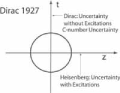
Figure 1: Space-time picture of quantum mechanics. There are quantum excitations along the space-like longitudinal direction, but there are no excitations along the time-like direction. The time-energy relation is a c-number uncertainty relation.

2.1 Dirac’s C-Number Time-Energy Uncertainty Relation

Even before Heisenberg formulated his uncertainty principle in 1927, Dirac studied the uncertainty relation applicable to the time and energy variables [7, 12]. This time-energy uncertainty relation was known before 1927 from the transition time and line broadening in atomic spectroscopy. As soon as Heisenberg formulated his uncertainty relation, Dirac considered whether the two uncertainty relations could be combined to form a Lorentz covariant uncertainty relation [7].

He noted one major difficulty. There are excitations along the space-like longitudinal direction starting from the position-momentum uncertainty, while there are no excitations along the time-like direction. The time variable is a c-number. How then can this space-time asymmetry be made consistent with Lorentz covariance, where the space and time coordinates are mixed up for moving observers.

Heisenberg’s uncertainty relation is applicable to space separation variables. For instance, the Bohr radius measures the difference between the proton and electron. Dirac never addressed the question of the separation in time variable or the time interval even in his later papers.

As for the space-time asymmetry, Dirac came back to this question in his 1949 paper [9] where he discusses the “instant form” of relativistic dynamics. He talks indirectly about the possibility of freezing three of the six parameters of the Lorentz group, and thus working only with the remaining free parameters.

This idea was presented earlier by Wigner [13, 14] who observed that the internal space-time symmetries of particles are dictated by his little groups with three independent parameters.

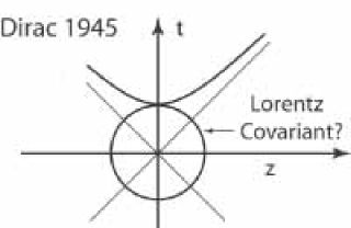
Figure 2: Dirac’s four-dimensional oscillators localized in a closed space-time region. This is not a Lorentz-invariant concept. How about Lorentz covariance?

2.2 Dirac’s four-dimensional oscillators

During World War II, Dirac was looking into the possibility of constructing representations of the Lorentz group using harmonic oscillator wave functions [8]. The Lorentz group is the language of special relativity, and the present form of quantum mechanics starts with harmonic oscillators. Therefore, he was interested in making quantum mechanics Lorentz-covariant by constructing representations of the Lorentz group using harmonic oscillators.

In his 1945 paper [8], Dirac considers the Gaussian form

$$\exp\left\{-{1\over 2}\left(x^{2}+y^{2}+z^{2}+t^{2}\right)\right\}.$$ (1)

We note that this Gaussian form is in the $(x,~{}y,~{}z,~{}t)$ coordinate variables. Thus, if we consider a Lorentz boost along the $z$ direction, we can drop the $x$ and $y$ variables, and write the above equation as

$$\exp\left\{-{1\over 2}\left(z^{2}+t^{2}\right)\right\}.$$ (2)

This is a strange expression for those who believe in Lorentz invariance where $\left(z^{2}-t^{2}\right)$ is an invariant quantity.

On the other hand, this expression is consistent with his earlier papers on the time-energy uncertainty relation [7]. In those papers, Dirac observed that there is a time-energy uncertainty relation, while there are no excitations along the time axis.

Let us look at Fig. 1 carefully. This figure is a pictorial representation of Dirac’s Eq.(2), with localization in both space and time coordinates. Then Dirac’s fundamental question would be how to make this figure covariant? This question is illustrated in Fig. 2. This is where Dirac stops. However, this is not the end of the Dirac story.

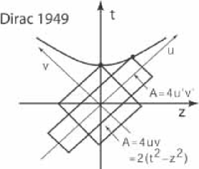
Figure 3: Lorentz boost in the light-cone coordinate system. The boost traces a point along the hyperbola. The boost also squeezes the square into a rectangle.

2.3 Dirac’s light-cone coordinate system

In 1949, the Reviews of Modern Physics published a special issue to celebrate Einstein’s 70th birthday. This issue contains Dirac paper entitled “Forms of Relativistic Dynamics” [9]. In this paper, he introduced his light-cone coordinate system, in which a Lorentz boost becomes a squeeze transformation, where one axis expands while the other contracts in such a way that their product remains invariant.

When the system is boosted along the $z$ direction, the transformation takes the form

$$\pmatrix{z^{\prime}\cr t^{\prime}}=\pmatrix{\cosh(\eta/2)&\sinh(\eta/2)\cr\sinh(\eta/2)&\cosh(\eta/2)}\pmatrix{z\cr t}.$$ (3)

This is not a rotation, and people still feel strange about this form of transformation. In 1949 [9], Dirac introduced his light-cone variables defined as [9]

$$u=(z+t)/\sqrt{2},\qquad v=(z-t)/\sqrt{2},$$ (4)

the boost transformation of Eq.(3) takes the form

$$u^{\prime}=e^{\eta/2}u,\qquad v^{\prime}=e^{-\eta/2}v.$$ (5)

The $u$ variable becomes expanded while the $v$ variable becomes contracted, as is illustrated in Fig. 3. Their product

$$uv={1\over 2}(z+t)(z-t)={1\over 2}\left(z^{2}-t^{2}\right)$$ (6)

remains invariant. Indeed, in Dirac’s picture, the Lorentz boost is a squeeze transformation.

2.4 Dirac’s Coupled Oscillators

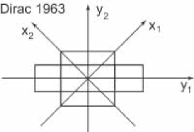
Figure 4: System of two coupled oscillators in the normal coordinate system. If the coupling becomes stronger, one coordinate variable becomes contracted while the other becomes expanded. However, the product of the two coordinates remains constant. This is an area-preserving transformation in this graph, just like Lorentz-boost in the light-cone coordinate system as described in Fig. 3.

In 1963 [10], Dirac published a paper on symmetries of coupled harmonic oscillators. Starting from step-up and step-down operators for the two oscillators, he was able to construct a representation of the deSitter group $O(3,2).$ Since this group contains two $O(3,1)$ Lorentz groups, we can extract Lorentz-covariance properties from his mathematics. It is even possible to extend this symmetry group to $O(3,3)$ to include damping effects of the oscillators.

In the present paper, we avoid group theory and use a set of two-by-two matrices to exploit the physical contents of Dirac’s 1963 paper. Let us start with the Hamiltonian for this system of two oscillators, which takes the form

$$H={1\over 2}\left\{{1\over m}_{1}p^{2}_{1}+{1\over m}_{2}p^{2}_{2}+Ax^{2}_{1}+Bx^{2}_{2}+Cx_{1}x_{2}\right\}.$$ (7)

It is possible to diagonalize by a single rotation the quadratic form of $x_{1}$ and $x_{2}$. However, the momentum variables undergo the same rotation. Therefore, the uncoupling of the potential energy by rotation alone will lead to a coupling of the two kinetic energy terms.

In order to avoid this complication, we have to bring the kinetic energy portion into a rotationally invariant form. For this purpose, we will need the transformation

$$\pmatrix{p^{\prime}_{1}\cr p^{\prime}_{2}}=\pmatrix{(m_{2}/m_{1})^{1/4}&0\cr 0&(m_{1}/m_{2})^{1/4}}\pmatrix{p_{1}\cr p_{2}}.$$ (8)

This transformation will change the kinetic energy portion to

$${1\over 2m}\left\{p^{\prime 2}_{1}+p^{\prime 2}_{2}\right\}$$ (9)

with $m=(m_{1}m_{2})^{1/2}$. This scale transformation does not leave the $x_{1}$ and $x_{2}$ variables invariant. If we insist on canonical transformations [15], the transformation becomes

$$\pmatrix{x^{\prime}_{1}\cr x^{\prime}_{2}}=\pmatrix{(m_{1}/m_{2})^{1/4}&0\cr 0&(m_{2}/m_{1})^{1/4}}\pmatrix{x_{1}\cr x_{2}}.$$ (10)

The scale transformations on the position variables are inversely proportional to those of their conjugate momentum variables. This is based on the Hamiltonian formalism where the position and momentum variables are independent variables.

On the other hand, in the Lagrangian formalism, where the momentum is proportional to the velocity which is the time derivative of the position coordinate, we have to apply the same scale transformation for both momentum and position variables [16]. In this case, the scale transformation takes the form

$$\pmatrix{x^{\prime}_{1}\cr x^{\prime}_{2}}=\pmatrix{(m_{2}/m_{1})^{1/4}&0\cr 0&(m_{1}/m_{2})^{1/4}}\pmatrix{x_{1}\cr x_{2}}.$$ (11)

With Eq.(8) for the momentum variables, this expression does not constitute a canonical transformation.

The canonical transformation leads to a unitary transformation in quantum mechanics. The issue of non-canonical transformation is not yet completely settled in quantum mechanics and is still an open question [15]. In either case, the Hamiltonian will take the form

$$H={1\over 2m}\left\{p^{2}_{1}+p^{2}_{2}\right\}+{1\over 2}\left\{Ax_{1}^{2}+Bx^{2}_{2}+Cx_{1}x_{2}\right\},$$ (12)

Here, we have deleted for simplicity the primes on the $x$ and $p$ variables.

We are now ready to decouple this Hamiltonian by making the coordinate rotation:

$$\pmatrix{y_{1}\cr y_{2}}=\pmatrix{\cos\alpha&-\sin\alpha\cr\sin\alpha&\cos\alpha}\pmatrix{x_{1}\cr x_{2}}.$$ (13)

Under this rotation, the kinetic energy portion of the Hamiltonian in Eq.(12) remains invariant. Thus we can achieve the decoupling by diagonalizing the potential energy. Indeed, the system becomes diagonal if the angle $\alpha$ becomes

$$\tan 2\alpha={C\over B-A}.$$ (14)

This diagonalization procedure is well known. What is new in this note is the introduction of the new parameters $K$ and $\eta$ defined as

$$K=\sqrt{AB-C^{2}/4},$$

$$\exp(\eta)=\frac{A+B+\sqrt{(A-B)^{2}+C^{2}}}{\sqrt{4AB-C^{2}}}.$$ (15)

In terms of this new set of variables, the Hamiltonian can be written as

$$H={1\over 2m}\left\{p^{2}_{1}+p^{2}_{2}\right\}+{K\over 2}\left\{e^{2\eta}y^{2}_{1}+e^{-2\eta}y^{2}_{2}\right\},$$ (16)

with

$$y_{1}=x_{1}\cos\alpha-x_{2}\sin\alpha,$$

$$y_{2}=x_{1}\sin\alpha+x_{2}\cos\alpha.$$ (17)

This completes the diagonalization process. The normal frequencies are

$$\omega_{1}=e^{\eta}\omega,\qquad\omega_{2}=e^{-\eta}\omega,$$ (18)

with

$$\omega=\sqrt{{K\over m}}.$$ (19)

This relatively new set of parameters has been discussed in in connection with Feynman’s rest of the universe [17].

Let us go back to Eq.(12) and Eq.(14). If $\alpha=0$, $C$ becomes zero and the oscillators become decoupled. If $\alpha=45^{o}$, then $A=B$, which means that the system consists of two identical oscillators coupled together by the $C$ term. In this case,

$$\exp{(\eta)}=\sqrt{\frac{2A+C}{2A-C}},\quad or\quad\eta=\frac{1}{2}\ln\left(\frac{2A+C}{2A-C}\right).$$ (20)

Thus $\eta$ measures the strength of the coupling.

The mathematics becomes very simple for $\alpha=45^{o}$, and this simple case can be applied to many physical problems, including the present problem of combining quantum mechanics with relativity. Indeed the $y_{1},y_{2}$ variables become

$$y_{1}=\frac{x_{1}-x_{2}}{\sqrt{2}},\qquad y_{2}=\frac{x_{1}+x_{2}}{\sqrt{2}}.$$ (21)

If $y_{1}$ and $y_{2}$ are measured in units of $(mK)^{1/4}$, the ground-state wave function of this oscillator system is

$$\psi_{\eta}(x_{1},x_{2})={1\over\sqrt{\pi}}\exp{\left\{-{1\over 2}(e^{\eta}y^{2}_{1}+e^{-\eta}y^{2}_{2})\right\}},$$ (22)

The wave function is separable in the $y_{1}$ and $y_{2}$ variables, when $\eta=0,$ remains separable while they are expanded and contracted by $e^{\eta/2}$ and $e^{-\eta/2}$ respectively as illustrated in Fig. 4.

On the other hand, for the variables $x_{1}$ and $x_{2}$, the wave function takes the form

$$\psi_{\eta}(x_{1},x_{2})={1\over\sqrt{\pi}}\exp\left\{-{1\over 4}\left[e^{\eta}(x_{1}-x_{2})^{2}+e^{-\eta}(x_{1}+x_{2})^{2}\right]\right\}.$$ (23)

In his 1963 paper [10], Dirac strictly worked with step-up and step-down operators. He made no attempt to use a normal coordinate system. It is indeed gratifying to translate his algebraic formulas into a geometry. Let us now compare Fig. 4 with Fig. 3. They are the same! Indeed, the geometry of Lorentz boost in Dirac’s light-cone coordinate system is identical to that of the coupled oscillators. The coupling constant is translated into the boost parameter as given in Eq.(20).

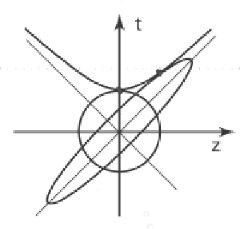
Figure 5: Effect of the Lorentz boost on the space-time wave function. The circular space-time distribution in the rest frame becomes Lorentz-squeezed to become an elliptic distribution.

3 Lorentz-covariant Picture of Quantum Bound States

If we combine Fig. 1 and Fig. 3, then we end up with Fig. 5. In mathematical formula, this transformation changes the Gaussian form of Eq.(2) into

$$\psi_{\eta}(z,t)=\left({1\over\pi}\right)^{1/2}\exp\left\{-{1\over 4}\left[e^{-\eta}(z+t)^{2}+e^{\eta}(z-t)^{2}\right]\right\}.$$ (24)

This formula together with Fig. 5 is known to describe all essential high-energy features observed in high-energy laboratories [3, 18, 19].

Indeed, this elliptic deformation explains one of the most controversial issues in high-energy physics. Hadrons are known to be bound states of quarks. Its bound-state quantum mechanics is assumed to be the same as that of the hydrogen atom. The question is how the hadron would look to an observer on a train. If the train moves with a speed close to that of light, the hadron appears like a collection of partons, according to Feynman [3]. Feynman’s partons have properties quite different from those of the quarks. For instance, they interact incoherently with external signals. The elliptic deformation property described in Fig. 5 explains that the quark and parton models are two different manifestations of the same covariant entity.

Quantum field theory has been quite successful in terms of Feynman diagrams based on the S-matrix formalism, but is useful only for physical processes where a set of free particles becomes another set of free particles after interaction. Quantum field theory does not address the question of localized probability distributions and their covariance under Lorentz transformations. In order to address this question, Feynman et al. suggested harmonic oscillators to tackle the problem [5]. Their idea is indicated in Fig. 6.

In this report, we are concerned with the quantum bound system, and we have examined the four-papers of Dirac on the question of making the uncertainty relations consistent with special relativity. Indeed, Dirac discussed this fundamental problem with mathematical devices which are both elegant and transparent.

Dirac of course noted that the time variable plays the essential role in the Lorentz-covariant world. On the other hand, he did not take into consideration the concept of time separation. When we talk about the hydrogen atom, we are concerned with the distance between the proton and electron. To a moving observer, there is also a time-separation between the two particles.

Instead of the hydrogen atom, we use these days the hadron consisting of two quarks bound together with an attractive force, and consider their space-time positions $x_{a}$ and $x_{b}$,and use the variables [5]

$$X=\frac{x_{a}+x_{b}}{2},\qquad x=\frac{x_{a}-x_{b}}{2\sqrt{2}}.$$ (25)

The four-vector $X$ specifies where the hadron is located in space and time, while the variable $x$ measures the space-time separation between the quarks. Let us call their time components $T$ and $t$. These variables actively participate in Lorentz transformations. The existence of the $T$ variable is known, but the Copenhagen school was not able to see the existence of this $t$ variable.

Paul A. M. Dirac was concerned with the time variable throughout his four papers discussed in this report. However, he did not make a distinction between the $T$ and $t$ variables. The $T$ variable ranges from $-\infty$ to $+\infty$, and is constantly increasing. On the other hand, the $t$ variable is the time interval, and remains unchanged in a given Lorentz frame.

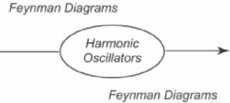
Figure 6: Feynman’s roadmap for combining quantum mechanics with special relativity. Feynman diagrams work for running waves, and they provide a satisfactory resolution for scattering states in Einstein’s world. For standing waves trapped inside an extended hadron, Feynman suggested harmonic oscillators as the first step.

Indeed, when Feynman et al. wrote down the Lorentz-invariant differential equation [5]

$${1\over 2}\left\{x^{2}_{\mu}-{\partial^{2}\over\partial x_{\mu}^{2}}\right\}\psi(x)=\lambda\psi(x),$$ (26)

$x_{\mu}$ was for the space-time separation between the quarks.

This four-dimensional differential equation has more than 200 forms of solutions depending on boundary conditions. However, there is only one set of solutions to which we can give a physical interpretation. Indeed, the Gaussian form of Eq.(1) is a solution of the above differential equation. If we boost the system along the $z$ direction, we can separate away the $x$ and $y$ components in the Gaussian form and write the wave function in the form of Eq.(2).

It is then possible to construct a representation of the Poincaré group from the solutions of the above differential equation [14]. If the system is boosted, the wave function becomes the Gaussian form given in Eq.(24), which becomes Eq.(2) if $\eta$ becomes zero. This wave function is also a solution of the Lorentz-invariant differential equation of Eq.(26). The transition from Eq.(2) to Eq.(24) is illustrated in Fig. 5.

4 Lorentz-covariant Quark Model

Early successes in the quark model includes the calculation of the ratio of the neutron and proton magnetic moments [20], and the hadronic mass spectra [5, 21]. These are based on hadrons at rest. We are interested in this paper how the hadrons in the quark model appear to observers in different Lorentz frames.

The idea that the proton or neutron has a space-time extension had been developed long before Gell-Mann’s proposal for the quark model [1]. Yukawa [22] developed this idea as early as 1953, and his idea was followed up by Markov, Ginzburg, and Man’ko [23, 24].

Since Einstein formulated special relativity for point particles, it has been and still is a challenge to formulate a theory for particles with space-time extensions. The most naive idea would be to study rigid spherical objects, and there were many papers on this subjects. But we do not know where that story stands these days. We can however replace these extended rigid bodies by extended wave packets or standing waves, thus by localized probability entities. Then what are the constituents within those localized waves? The quark model gives the natural answer to this question.

The first experimental discovery of the non-zero size of the proton was made by Hofstadter and McAllister [25], who used electron-proton scattering to measure the charge distribution inside the proton. If the proton were a point particle, the scattering amplitude would just be a Rutherford formula. However, Hofstadter and MacAllister found a tangible departure from this formula which can only be explained by a spread-out charge distribution inside the proton.

In this section, we are interested in how well the bound-state picture developed in Sec. 4 works in explaining relativistic phenomena of hadrons, specifically the proton. The Lorentz-covariant model of Sec. 3 is of course based on Dirac’s four papers discussed in Sec. 2.

First, we show that the static quark model and Feynman’s parton picture are two limiting cases of one Lorentz-covariant entity. In the quark model, the hadron appears like quantum bound states with discrete energy spectra. In the parton model, the rapidly moving hadron appears like a collection of infinite number of free independent particles. Can these be explained with one theory? This is what we would like to address in subsection 4.1.

As for the case between these two limits, we discuss the hadronic form factor which occupies an important place in every theoretical model in strong interactions since Hofstadter’s discovery in 1955 [25]. The key question is the proton form factor decreases as 1/(momentum transfer$)^{4}$ as the momentum transfer becomes large. This is called the dipole cut-off in the literature. We shall see in subsection 4.2 that the covariant model of Sec. 3 gives this dipole cut-off for spinless quarks.

4.1 Feynman’s Parton Picture

In a hydrogen atom or a hadron consisting of two quarks, there is a spacial separation between two constituent elements. In the case of the hydrogen atom we call it the Bohr radius. If the atom or hadron is at rest, the time-separation variable does not play any visible role in quantum mechanics. However, if the system is boosted to the Lorentz frame which moves with a speed close to that of light, this time-separation variable becomes as important as the space separation of the Bohr radius. Thus, the time-separation variable plays a visible role in high-energy physics which studies fast-moving bound states. Let us study this problem in more detail.

It is a widely accepted view that hadrons are quantum bound states of quarks having a localized probability distribution. As in all bound-state cases, this localization condition is responsible for the existence of discrete mass spectra. The most convincing evidence for this bound-state picture is the hadronic mass spectra [5, 14].

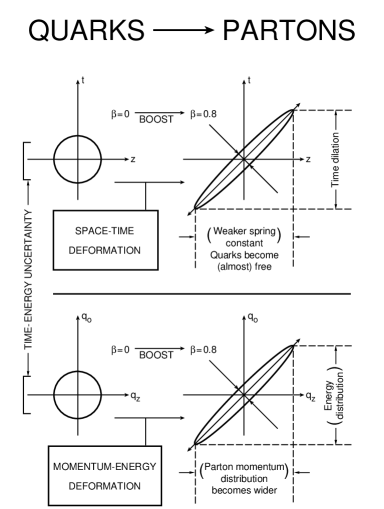
Figure 7: Lorentz-squeezed space-time and momentum-energy wave functions. As the hadron’s speed approaches that of light, both wave functions become concentrated along their respective positive light-cone axes. These light-cone concentrations lead to Feynman’s parton picture.

However, this picture of bound states is applicable only to observers in the Lorentz frame in which the hadron is at rest. How would the hadrons appear to observers in other Lorentz frames?

In 1969, Feynman observed that a fast-moving hadron can be regarded as a collection of many “partons” whose properties appear to be quite different from those of the quarks [3, 14]. For example, the number of quarks inside a static proton is three, while the number of partons in a rapidly moving proton appears to be infinite. The question then is how the proton looking like a bound state of quarks to one observer can appear different to an observer in a different Lorentz frame? Feynman made the following systematic observations.

• The picture is valid only for hadrons moving with velocity close to that of light.

• The interaction time between the quarks becomes dilated, and partons behave as free independent particles.

• The momentum distribution of partons becomes widespread as the hadron moves fast.

• The number of partons seems to be infinite or much larger than that of quarks.

Because the hadron is believed to be a bound state of two or three quarks, each of the above phenomena appears as a paradox, particularly b) and c) together. How can a free particle have a wide-spread momentum distribution?

In order to resolve this paradox, let us construct the momentum-energy wave function corresponding to Eq.(24). If the quarks have the four-momenta $p_{a}$ and $p_{b}$, we can construct two independent four-momentum variables [5]

$$P=p_{a}+p_{b},\qquad q=\sqrt{2}(p_{a}-p_{b}).$$ (27)

The four-momentum $P$ is the total four-momentum and is thus the hadronic four-momentum. $q$ measures the four-momentum separation between the quarks. Their light-cone variables are

$$q_{u}=(q_{0}-q_{z})/\sqrt{2},\qquad q_{v}=(q_{0}+q_{z})/\sqrt{2}.$$ (28)

The resulting momentum-energy wave function is

$$\phi_{\eta}(q_{z},q_{0})=\left({1\over\pi}\right)^{1/2}\exp\left\{-{1\over 2}\left[e^{-2\eta}q_{u}^{2}+e^{2\eta}q_{v}^{2}\right]\right\}.$$ (29)

Because we are using here the harmonic oscillator, the mathematical form of the above momentum-energy wave function is identical to that of the space-time wave function of Eq.(24). The Lorentz squeeze properties of these wave functions are also the same. This aspect of the squeeze has been exhaustively discussed in the literature [14, 18, 26], and they are illustrated again in Fig. 7 of the present paper. The hadronic structure function calculated from this formalism is in a reasonable agreement with the experimental data [27].

When the hadron is at rest with $\eta=0$, both wave functions behave like those for the static bound state of quarks. As $\eta$ increases, the wave functions become continuously squeezed until they become concentrated along their respective positive light-cone axes. Let us look at the z-axis projection of the space-time wave function. Indeed, the width of the quark distribution increases as the hadronic speed approaches that of the speed of light. The position of each quark appears widespread to the observer in the laboratory frame, and the quarks appear like free particles.

The momentum-energy wave function is just like the space-time wave function. The longitudinal momentum distribution becomes wide-spread as the hadronic speed approaches the velocity of light. This is in contradiction with our expectation from nonrelativistic quantum mechanics that the width of the momentum distribution is inversely proportional to that of the position wave function. Our expectation is that if the quarks are free, they must have their sharply defined momenta, not a wide-spread distribution.

However, according to our Lorentz-squeezed space-time and momentum-energy wave functions, the space-time width and the momentum-energy width increase in the same direction as the hadron is boosted. This is of course an effect of Lorentz covariance. This indeed leads to the resolution of one of the the quark-parton puzzles [14, 18, 26].

Another puzzling problem in the parton picture is that partons appear as incoherent particles, while quarks are coherent when the hadron is at rest. Does this mean that the coherence is destroyed by the Lorentz boost? The answer is NO, and here is the resolution to this puzzle.

When the hadron is boosted, the hadronic matter becomes squeezed and becomes concentrated in the elliptic region along the positive light-cone axis. The length of the major axis becomes expanded by $e^{\eta}$, and the minor axis is contracted by $e^{\eta}$.

This means that the interaction time of the quarks among themselves becomes dilated. Because the wave function becomes wide-spread, the distance between one end of the harmonic oscillator well and the other end increases. This effect, first noted by Feynman [2, 3], is universally observed in high-energy hadronic experiments. The period of oscillation increases like $e^{\eta}$.

On the other hand, the external signal, since it is moving in the direction opposite to the direction of the hadron, travels along the negative light-cone axis.

If the hadron contracts along the negative light-cone axis, the interaction time decreases by $e^{-\eta}$. The ratio of the interaction time to the oscillator period becomes $e^{-2\eta}$. The energy of each proton coming out of the Fermilab accelerator is $900GeV$. This leads the ratio to $10^{-6}$. This is indeed a small number. The external signal is not able to sense the interaction of the quarks among themselves inside the hadron.

Indeed, Feynman’s parton picture is one concrete physical example where the decoherence effect is observed. As for the entropy, the time-separation variable belongs to the rest of the universe. Because we are not able to observe this variable, the entropy increases as the hadron is boosted to exhibit the parton effect. The decoherence is thus accompanied by an entropy increase.

Let us go back to the coupled-oscillator system. The light-cone variables in Eq.(24) correspond to the normal coordinates in the coupled-oscillator system given in Eq.(16). According to Feynman’s parton picture, the decoherence mechanism is determined by the ratio of widths of the wave function along the two normal coordinates.

This decoherence mechanism observed in Feynman’s parton picture is quite different from other decoherences discussed in the literature. It is widely understood that the word decoherence is the loss of coherence within a system. On the other hand, Feynman’s decoherence discussed in this section comes from the way the external signal interacts with the internal constituents.

4.2 Nucleon Form Factors

Let us first see what effect the charge distribution has on the scattering amplitude, using nonrelativistic scattering in the Born approximation. If we scatter electrons from a fixed charge distribution whose density is $e\rho(r)$, the scattering amplitude is

$$f(\theta)=-\left(\frac{e^{2}m}{2\pi}\right)\int d^{3}xd^{3}x^{\prime}\frac{\rho(r^{\prime})}{R}\exp{(-i{\bf Q}\cdot{\bf x})},$$ (30)

where $r=|{\bf x}|,R=|{\bf r}-{\bf r^{\prime}}|,$ and ${\bf Q}={\bf K_{f}}-{\bf K_{i}},$ which is the momentum transfer. This amplitude can be reduced to

$$f(\theta)=\frac{2me^{2}}{Q^{2}}F(Q^{2}).$$ (31)

$F(Q^{2})$ is the Fourier transform of the density function which can be written as

$$F\left(Q^{2}\right)=\int d^{3}x\rho(r)\exp{(-i{\bf Q}\cdot{\bf x})}.$$ (32)

The above quantity is called the form factor. It describes the charge distribution in terms of the momentum transfer. The charge density is normalized:

$$\int\rho(r)d^{3}x=1.$$ (33)

Then F(0) = 1 from Eq.(32). If the density function is a delta function corresponding to a point charge, $F\left(Q^{2}\right)=1$ for all values of $Q^{2},$ then the scattering amplitude of Eq.(30) becomes the Rutherford formula for Coulomb scattering. The deviations from Rutherford scattering for increasing values of $Q^{2}$ give a measure of the charge distribution. This was precisely what Hofstadter’s experiment on the scattering of electrons from a proton target found. [25].

As the energy of incoming electrons becomes higher, we have to take into account the recoil effect of target protons, and formulate the problem relativistically. It is generally agreed that electrons and their electromagnetic interaction can be described by quantum electrodynamics, in which the method of perturbation theory using Feynman diagrams is often employed for practical calculations [28, 29]. In this perturbation approach, the scattering amplitude is expanded in power series of the fine structure constant $\alpha.$ Therefore, in lowest order in $\alpha,$ we can describe the scattering of an electron by a proton using the diagram given in Fig.(8). The corresponding matrix element is given in many textbooks on elementary particle physics [30]. It is proportional to

$$\bar{U}\left(P_{f}\right)\Gamma_{\mu}\left(P_{f},P_{i}\right)\left(\frac{1}{Q^{2}}\right)\bar{U}\left(K_{f}\right)\gamma^{\mu}U\left(K_{i}\right),$$ (34)

where $P_{i},P_{f},K_{i}$ and $K_{f}$ are the initial and final four-momenta of the proton and electron respectively. $U\left(P_{i}\right)$ is the Dirac spinor for the initial proton. $Q^{2}$ is the (four-momentum transfer$)^{4}$ and is

$$Q^{2}=\left(P_{f}-P_{i}\right)^{2}=\left(K_{f}-K_{i}\right)^{2}.$$ (35)

The $\left(1/Q^{2}\right)$ factor in Eq.(34) comes from the virtual photon being exchanged between the electron and the proton. It is customary to use the letter t for $Q^{2}$ in form factor studies, and this t should not be confused with the time separation variable. In the metric we use, this quantity is positive for physical values of the four-momenta for the particles involved in the scattering process.

Figure 8: Breit frame for electron-nucleon scattering. The momentum of the outgoing nucleon is equal in magnitude but opposite in sign to that of the incoming nucleon.

In order to make a relativistic calculation of the form factor, let us go back to the definition of the form factor given in Eq.(32). The density function depends only on the target particle, and is proportional to $\psi(x)^{\dagger}\psi(x)$, where $\psi(x)$ is the wave function for quarks inside the proton. This expression is a special case of the more general form

$$\rho(x)=\psi_{f}^{\dagger}(x)\psi_{i}(x),$$ (36)

where $\psi_{i}$ and $\psi_{f}$ are the initial and final wave function of the target atom. Indeed, the form factor of Eq.(32) can be written as

$$F\left(Q^{2}\right)=\left(\psi_{f}(x),e^{-i{\bf Q}\cdot{\bf r}}\psi_{i}(x)\right).$$ (37)

Starting from this expression, we can make the required Lorentz generalization using the relativistic wave functions for hadrons.

In order to see the details of the transition to relativistic physics, we should be able to replace each quantity in the expression of Eq.(32) by its relativistic counterpart. Let us go to the Lorentz frame in which the momenta of the incoming and outgoing nucleons have equal magnitude but opposite signs.

$${\bf p_{i}}+{\bf p_{f}}=0.$$ (38)

This kinematical condition is illustrated in Fig. 8.

The Lorentz frame in which the above condition holds is usually called the Breit frame. We assume without loss of generality that the proton comes along the $z$ direction before the collision and goes out along the negative $z$ direction after the scattering process, as illustrated in Fig. 8. In this frame, the four vector $Q=(K_{f}-K_{i})=(P_{i}-P_{f})$ has no time-like component. Thus the exponential factor ${\bf Q}\cdot{\bf r}$ can be replaced by the Lorentz-invariant form $Q\cdot x$. As for the wave functions for the protons, we can use the covariant harmonic oscillator wave functions discussed in this paper assuming that the nucleons are in the ground state. Then the only difference between the nonrelativistic and relativistic cases is that the integral in the evaluation of Eq.(32) is four-dimensional, including that for the time-like direction. This integral in the time-separation variable does not interfere with the exponential factor which does not depend on the time-separation variable.

Let us now write down the integral:

$$g\left(Q^{2}\right)=\int d^{4}x\psi^{\dagger}_{-\beta}(x)\psi_{\beta}(x)\exp{(-iQ\cdot x)}.$$ (39)

where $\beta$ is the velocity parameter for the incoming proton, and the wave function $\psi_{\beta}$ takes the form:

$$\psi_{\beta}(x)=\frac{1}{\pi}\exp{\left\{-\frac{x^{2}+y^{2}}{2}\right\}}$$

$$\hskip 28.45274pt\times\exp{\left\{-\frac{1}{4}\left[\frac{1-\beta}{1+\beta}(z+t)^{2}+\frac{1+\beta}{1-\beta}(z-t)^{2}\right]\right\}}.$$ (40)

After the above decomposition of the wave functions, we can perform the integrations in the $x$ and $y$ variables trivially. After dropping these trivial factors, we can write the product of the two wave functions as

$$\psi^{\dagger}_{-\beta}(x)\psi_{\beta}(x)=\frac{1}{\pi}\exp{\left\{-\left(\frac{1+\beta^{2}}{1-\beta^{2}}\right)\left(t^{2}+z^{2}\right)\right\}}.$$ (41)

Thus the $z$ and $t$ variables have been separated. Since the exponential factor in Eq.(32) does not depend on $t$, the $t$ integral in Eq.(39) can also be trivially performed, and the integral of Eq.(39) can be written as

$$g\left(Q^{2}\right)=\sqrt{\frac{1}{\pi}\left(\frac{1-\beta^{2}}{1+\beta^{2}}\right)}\int dze^{-2iPz}\exp{\left\{-\frac{1+\beta^{2}}{1-\beta^{2}}z^{2}\right\}},$$ (42)

where $P$ is the $z$ component of the momentum of the incoming nucleon. The (momentum transfer$)^{2}$ variable $Q^{2}$ is $4P^{2}.$ Indeed, the distribution of the hadronic material along the longitudinal direction became contracted [31].

We note that $\beta$ can be written as

$$\beta^{2}=\frac{Q^{2}}{Q^{2}+4M^{2}},$$ (43)

where $M$ is the proton mass. This equation tells $\beta=0$ when $Q^{2}=0$, while it becomes one as $Q^{2}$ becomes infinity.

The evaluation of the above integral for $g\left(Q^{2}\right)$ in Eq.(42) leads to

$$g\left(Q^{2}\right)=\left(\frac{2M^{2}}{Q^{2}+2M^{2}}\right)\exp{\left\{\frac{-Q^{2}}{2(Q^{2}+2M^{2})}\right\}}.$$ (44)

For $Q^{2}=0,$ the above expression becomes 1. It decreases as

$$g\left(Q^{2}\right)\sim\frac{1}{Q^{2}}$$ (45)

for large values of $Q^{2}.$

We have so far carried out the calculation for an oscillator bound state of two quarks. The proton consists of three quarks. As shown in the paper of Feynman et al. [5], the problem becomes a product of two oscillator modes. Thus, the generalization of the above calculation to the three-quark system is straightforward, and the result is that the form factor $G\left(Q^{2}\right)$ takes the form

$$G\left(Q^{2}\right)=\left(\frac{2M^{2}}{Q^{2}+2M^{2}}\right)^{2}\exp{\left\{\frac{-Q^{2}}{\left(Q^{2}+2M^{2}\right)}\right\}}.$$ (46)

which is 1 at $Q^{2}=0$, and decreases as

$$G\left(Q^{2}\right)\sim\left[\frac{1}{Q^{2}}\right]^{2}$$ (47)

for large values of $Q^{2}.$ Indeed, this function satisfies the requirement of the “dipole-cut-off” behavior for of the form factors, which has been observed in high-energy laboratories. This calculation was carried first by Fujimura et al. in 1970 [32].

Let us re-examine the above calculation. If we replace $\beta$ by zero in Eq.(42) and ignore the elliptic deformation of the wave functions, $g\left(Q^{2}\right)$ will become

$$g\left(Q^{2}\right)=e^{-Q^{2}/4},$$ (48)

which will leads to an exponential cut-off of the form factor. This is not what we observe in laboratories.

In order to gain a deeper understanding of the above-mentioned correlation, let us study the case using the momentum-energy wave functions:

$$\phi_{\beta}(q)=\left(\frac{1}{\pi}\right)^{2}\int d^{4}e^{-iq\cdot x}\psi_{\beta}(x).$$ (49)

As before, we can ignore the transverse components. Then $g\left(Q^{2}\right)$ can be written as [14]

$$\int dq_{0}dq_{z}\phi^{*}_{\beta}\left(q_{0},q_{z}-P\right)\phi_{\beta}\left(q_{0},q_{z}+P\right).$$ (50)

We have sketched the above overlap integral in Fig. 9. When $Q^{2}=0$ or $P=0$, the two wave functions overlap completely in the $q_{z}q_{0}$ plane. As P increases, the wave functions become separated. However, they maintain a small overlapping region due to the elliptic or squeeze deformation seen in Fig. 5. In the non-relativistic case, where the deformation is not taken into account, there is no overlapping region as seen in Fig. 9. This is precisely why the relativistic calculation gives a slower decrease in $Q^{2}$ than in the nonrelativistic case.

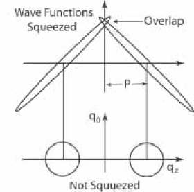
Figure 9: Lorentz-Dirac deformation of the momentum-energy wave functions in the form factor calculation. As the momentum transfer increases, the two wave functions become separated. In the relativistic case, the wave functions maintain an overlapping region. Wave functions become completely separated in the nonrelativistic calculation. This lack of overlapping region leads to an unacceptable behavior of the form factor.

We have so far been interested only in the space-time behavior of the hadronic wave function. We should not forget the fact that quarks are spin-1/2 particles. The effect of this spin manifests itself prominently in the baryonic mass spectra. Since we are concerned here with the relativistic effects, we have to construct a relativistic spin wave function for the quarks. This quark wave function should give the hadronic spin wave function. In the case of nucleons, the quark spins should be combined in a manner to generate the form factor of Eq.(41).

The naive approach to this problem is to use free Dirac spinors for the quarks. However, it was shown by Lipes [33] that the use of free-particle Dirac spinors leads to a wrong form factor behavior. Since quarks in a hadron are not free particles, Lipes’s result does not alarm us. The difficult problem is to find a suitable mechanism in which quark spins are coupled to orbital motion in a relativistic manner. This is a nontrivial research problem, and further study is needed along this direction [34].

In addition, there are recent experimental results which indicate departure from the dipole behavior of Eq.(47) [35]. In addition, there have been other theoretical attempts to calculate the proton form factor. Yes, whenever a new theoretical model appears, there appears a new attempt to calculate the form factor. In the past, there were many attempts to calculate this quantity in the framework of quantum field theory, without much success.

In 1960, Frazer and Fulco calculated the form factor using the technique of dispersion relations [36]. In so doing they had to assume the existence of the so-called $\rho$ meson, which was later found experimentally, and which subsequently played a pivotal role in the development of the quark model.

Even these days, the form factor calculation occupies a very important place in recent theoretical models, such as QCD lattice theory [37] and the Faddeev equation [38]. However, it is still noteworthy that Dirac’s form of Lorentz-covariant bound states leads to the essential dipole cut-off behavior of the proton form factor.

Conclusion

The hydrogen atom played a pivotal role in the development of quantum mechanics. Quantum mechanics had to be formulated to explain its discrete energy spectra, radiation decay rates, as well as the scattering of electrons by the proton.

The quark model still plays the central role in present-day high-energy physics. The model can explain the hadronc mass spectra, hadronic structure, and hadronic decay rates. In addition we are dealing with hadrons which appear as quantum bound states when they are at rest, how would they appear to observes in different frames, particularly in the frame moving with a velocity close to that of light. It was Feynman who proposed the parton model to describe those high-energy hadrons.

In this model, we have presented a Lorentz-covariant model which gives both the quark model and the parton model as two limiting cases. In addition we discussed the form factor as the case between these limits.

In constructing the Lorentz-covariant model, we noted Paul A. M. Dirac made life-long efforts to make quantum mechanics consistent with special relativity. We have chosen four of his papers and combined them to construct a consistent theory. It was like building a canal. The easiest way to build the canal is to link up the existing lakes. Dirac indeed dug four big lakes. It is a gratifying experience to link them up.

Dirac constructed those lakes in order to study whether the Copenhagen school of quantum mechanics can be made consistent with Einstein’s Lorentz-covariant world.

After studying Dirac’s papers, we arrived at the conclusion that the Copenhagen school completely forgot to take into account the question of simultaneity and time separation [4]. The question then is whether the localized probability distribution can be made consistent with Einstein’s Lorentz covariance. We have addressed this question in this paper.

References

- [1] Gell-Mann, M. Phys. Lett 1964, 13, 598-602.
- [2] Feynman, R. P. Phys. Rev. Lett. 1969, 23 1415-1417.
- [3] Feynman, R. P. The Behavior of Hadron Collisions at Extreme Energies; in High Energy Collisions, Proceedings of the Third International Conference, Stony Brook, NY; Yang, C. N.; et al.; Eds.; Gordon and Breach: New York, NY 1969, pp 237-249.
- [4] Kim, Y. S.; Noz, M. E. The Question of Simultaneity in Relativity and Quantum Mechanics; in QUANTUM THEORY: Reconsideration of Foundations - 3; Adenier, G; Khrennikov, A.; Nieuwenhuizen, T. M. Eds.; AIP Conference Proceedings; American Institute of Physics: College Park, MD,2006; 810, pp. 168-178.
- [5] Feynman, R. P.; Kislinger, M.; Ravndal, F. Phys. Rev. D 1971, 3, 2706-2732.
- [6] Dirac, P. A. M. Physics Today 1970, 23, No. 4, 29-31.
- [7] Dirac, P. A. M. Proc. Roy. Soc. (London) 1927, A114, 243-265.
- [8] Dirac, P. A. M. Proc. Roy. Soc. (London) 1945, A183, 284-295.
- [9] Dirac, P. A. M. Rev. Mod. Phys. 1949, 21, 392-399.
- [10] Dirac, P. A. M. J. Math. Phys. 1963, 4, 901-909.
- [11] Kim, Y. S.; Noz, M. E. Phase Space Picture of Quantum Mechanics; World Scientific Publishing Company: Singapore, 1991.
- [12] Wigner, E. P. On the Time-Energy Uncertainty Relation; in Aspects of Quantum Theory; Salam, A.; Wigner, E. P. Eds.; Cambridge University Press: London, England, 1972; pp 237-247.
- [13] Wigner, E. Ann. Math. 1939, 40, 149-204.
- [14] Kim, Y. S.; Noz, M. E. Theory and Applications of the Poincaré Group; D. Reidel Publishing Company: Dordrecht, The Netherlands, 1986.
- [15] Han, D.; Kim,Y. S.; Noz, M. E. J. Math. Phys. 1995, 36, 3940-3954.
- [16] Aravind, P. K. Am. J. Phys. 1989, 57,309-311.
- [17] Han, D.; Kim, Y. S.; Noz, M. E. Am. J. Phys. 1999, 67,61-66.
- [18] Kim, Y. S.; Noz, M. E. Phys. Rev. D 1977, 15, 335-338.
- [19] Kim, Y. S.; Noz, M. E. J. Opt. B: Quantum and Semiclass. Opt. 2005,7 S458-S467.
- [20] Beg, M. A. B; Lee, B. W.; Pais, A. Phys. Rev. Lett. 1964, 13 514-517
- [21] Greenberg, O. W.; Resnikoff, M. Phys. Rev. 1967, 1844-1851
- [22] Yukawa, H. Phys. Rev. 1953, 91 415-416.
- [23] Markov, M. Suppl. Nuovo Cimento 1956, 3, 760-772.
- [24] Ginzburg, V. L.; Man’ko, V. I. Nucl. Phys. 1965, 74 577-588
- [25] Hofstadter, R; McAllister, R. W. Phys. Rev. 1955, 98 217-218.
- [26] Kim, Y. S. Phys. Rev. Lett. 1989, 63, 348-351.
- [27] Hussar, P. E. Phys. Rev. D 1981, 23 2781-2783.
- [28] Schweber, S. S. An Introduction to Relativistic Quantum Field Theory;Row-Peterson: Elmsford, NY, 1961.
- [29] Itzykson, C.; Zuber, J. B. Quantum Field Theory; McGraw-Hill: New York,NY, 1980.
- [30] Frazer, W. Elementary Particle Physics; Prentice Hall: Englewood Cliffs, NJ, 1966.
- [31] Licht, A. L.; Pagnamenta,A. Phys. Rev. D 1970, 2, 1150-1156; 1156-1160.
- [32] Fujimura, K; Kobayashi, T; Namiki, M. Prog. Theor. Phys. 1970, 43 73-79.
- [33] Lipes, R. Phys. Rev. D. 1972, 5 2948-2863.
- [34] Henriques, A. B.; Keller, B. H.; Moorhouse, R. G. 1975 Ann. Phys. (NY) 93 125-151.
- [35] Punjabi, V; Perdrisat, C. F.; et al. Phys.Rev C 2005, 71 055202-27; Erratum-ibid. C 2005 71 069902.
- [36] Frazer, W.; Fulco, J. Phys. Rev. Lett. 1960, 2 365-368.
- [37] Matevosyan, H. H.; Thomas, A. W.; Miller, G. A. Phys.Rev. 2005, C72 065204-5.
- [38] Alkofer, R; Holl, A; Kloker, M; Karssnigg A.; Roberts, C. D. Few-Body Systems 2005, 37 1-31.