Deconvolution of confocal microscopy images using proximal iteration and sparse representations

Abstract

We propose a deconvolution algorithm for images blurred and degraded by a Poisson noise. The algorithm uses a fast proximal backward-forward splitting iteration. This iteration minimizes an energy which combines a non-linear data fidelity term, adapted to Poisson noise, and a non-smooth sparsity-promoting regularization (e.g $\ell_{1}$-norm) over the image representation coefficients in some dictionary of transforms (e.g. wavelets, curvelets). Our results on simulated microscopy images of neurons and cells are confronted to some state-of-the-art algorithms. They show that our approach is very competitive, and as expected, the importance of the non-linearity due to Poisson noise is more salient at low and medium intensities. Finally an experiment on real fluorescent confocal microscopy data is reported.

Index Terms—  Deconvolution, Poisson noise, Confocal microscopy, Iterative thresholding, Sparse representations.

1 Introduction

Fluorescent microscopy suffers from two main sources of degradation: the optical system and the acquisition noise. The optical system has a finite resolution introducing a blur in the observation. This degradation is modeled as convolution with the point spread function (PSF). The second source of image degradation is due to Poisson count process (shot noise). In presence of Poisson noise, several deconvolution algorithms have been proposed such as the well-known Richardson-Lucy (RL) algorithm or Tikhonov-Miller inverse filter, to name a few. RL is extensively used for its good adaptation to Poisson noise, but it tends to amplify noise after a few iterations. Regularization can be introduced in order to avoid this issue. In biological imaging deconvolution, many kinds of regularization have been suggested: total variation with RL [1] which gives staircase artifacts, Tikhonov with RL (see [2] for a review), etc. Wavelets have also been used as a regularization scheme when deconvolving biomedical images; [3] presents a version of RL combined with wavelets denoising, and [4] use the thresholded Landweber iteration of [5]. The latter approach implicitly assumes that the contaminating noise is Gaussian.

In the context of deconvolution with Gaussian white noise, sparsity-promoting regularization over orthogonal wavelet coefficients has been recently proposed [5, 6]. Generalization to frames was proposed in [7, 8]. In [9], the authors presented an image deconvolution algorithm by iterative thresholding in an overcomplete dictionary of transforms. However, all sparsity-based approaches published so far have mainly focused on Gaussian noise.

In this paper, we propose an image deconvolution algorithm for data blurred and contaminated by Poisson noise. The Poisson noise is handled properly by using the Anscombe variance stabilizing transform (VST), leading to a non-linear degradation equation with additive Gaussian noise, see (2). The deconvolution problem is then formulated as the minimization of a convex functional with a non-linear data-fidelity term reflecting the noise properties, and a non-smooth sparsity-promoting penalty over representation coefficients of the image to restore, e.g. wavelet or curvelet coefficients. Inspired by the work in [6], a fast proximal iterative algorithm is proposed to solve the minimization problem. Experimental results are carried out to compare our approach on a set of simulated and real confocal microscopy images, and show the striking benefits gained from taking into account the Poisson nature of the noise and the morphological structures involved in the image.

Notation

Let $\mathcal{H}$ a real Hilbert space, here a finite dimensional vector subspace of $\mathbb{R}^{n}$. We denote by $\left\|.\right\|_{2}$ the norm associated with the inner product in $\mathcal{H}$, and $\mathbf{I}$ is the identity operator on $\mathcal{H}$. ${x}$ and ${{\alpha}}$ are respectively reordered vectors of image samples and transform coefficients. A function $f$ is coercive, if $\lim_{\left\|{x}\right\|_{2}\rightarrow+\infty}f\left({{x}}\right)=+\infty$. $\Gamma_{0}(\mathcal{H})$ is the class of all proper lower semi-continuous convex functions from $\mathcal{H}$ to $]-\infty,+\infty]$.

2 Problem statement

Consider the image formation model where an input image ${x}$ is blurred by a point spread function (PSF) $h$ and contaminated by Poisson noise. The observed image is then a discrete collection of counts $y=(y_{i})_{1\leqslant i\leqslant n}$ where $n$ is the number of pixels. Each count $y_{i}$ is a realization of an independent Poisson random variable with a mean $(h\circledast x)_{i}$, where $\circledast$ is the circular convolution operator. Formally, this writes $y_{i}\sim\mathcal{P}\left({(h\circledast x)_{i}}\right)$.

A naive solution to this deconvolution problem would be to apply traditional approaches designed for Gaussian noise. But this would be awkward as (i) the noise tends to Gaussian only for large mean $(h\circledast x)_{i}$ (central limit theorem), and (ii) the noise variance depends on the mean anyway. A more adapted way would be to adopt a bayesian framework with an appropriate anti-log-likelihood score reflecting the Poisson statistics of the noise. Unfortunately, doing so, we would end-up with a functional which does not satisfy some key properties (the Lipschitzian property stated after (3)), hence preventing us from using the backward-forward splitting proximal algorithm to solve the optimization problem. To circumvent this difficulty, we propose to handle the noise statistical properties by using the Anscombe VST defined as

$$z_{i}=2\sqrt{y_{i}+\tfrac{3}{8}},~{}1\leqslant i\leqslant n.$$ (1)

Some previous authors [10] have already suggested to use the Anscombe VST, and then deconvolve with wavelet-domain regularization as if the stabilized observation $z_{i}$ were linearly degraded by $h$ and contaminated by additive Gaussian noise. But this is not valid as standard asymptotic results of the Anscombe VST state that

$$z_{i}=2\sqrt{(h\circledast x)_{i}+\tfrac{3}{8}}+\varepsilon,\quad\varepsilon\sim\mathcal{N}(0,1)$$ (2)

where $\varepsilon$ is an additive white Gaussian noise of unit variance. In words, $z$ is non-linearly related to $x$. In Section 4, we provide an elegant optimization problem and a fixed point algorithm taking into account such a non-linearity.

3 Sparse image representation

Let $x\in\mathcal{H}$ be an $\sqrt{n}\times\sqrt{n}$ image. $x$ can be written as the superposition of elementary atoms $\varphi_{\gamma}$ parametrized by $\gamma\in\mathcal{I}$ such that $x=\sum_{\gamma\in\mathcal{I}}\alpha_{\gamma}\varphi_{\gamma}=\Phi{{\alpha}},\quad\left|\mathcal{I}\right|=L,~{}L\geqslant n$. We denote by $\Phi$ the dictionary i.e. the $n\times L$ matrix whose columns are the generating waveforms $\left({\varphi_{\gamma}}\right)_{\gamma\in\mathcal{I}}$ all normalized to a unit $\ell_{2}$-norm. The forward transform is then defined by a non-necessarily square matrix $\mathbf{T}=\Phi^{\mathrm{T}}\in\mathbb{R}^{L\times n}$. In the rest of the paper, $\Phi$ will be an orthobasis or a tight frame with constant $A$.

4 Sparse Iterative Deconvolution

4.1 Optimization problem

The class of minimization problems we are interested in can be stated in the general form [6]:

$$\operatorname*{arg\ min}_{x\in\mathcal{H}}f_{1}(x)+f_{2}(x).$$ (3)

where $f_{1}\in\Gamma_{0}(\mathcal{H})$, $f_{2}\in\Gamma_{0}(\mathcal{H})$ and $f_{1}$ is differentiable with $\kappa$-Lipschitz gradient. We denote by $\mathcal{M}$ the set of solutions.

From (2), we immediately deduce the data fidelity term

$$F\circ H\circ\Phi~{}({{\alpha}}),~{}\text{with}$$ (4)

$$F:\eta\mapsto\sum_{i=1}^{n}f(\eta_{i}),\quad f(\eta_{i})=\frac{1}{2}\left(z_{i}-2\sqrt{\eta_{i}+\tfrac{3}{8}}\right)^{2},$$

where $H$ denotes the convolution operator. From a statistical perspective, (4) corresponds to the anti-log-likelihood score.

Adopting a bayesian framework and using a standard maximum a posteriori (MAP) rule, our goal is to minimize the following functional with respect to the representation coefficients $\alpha$:

$$(\mathsf{P}_{\lambda,\psi}):\operatorname*{arg\ min}_{\alpha}J(\alpha)$$ (5)

$$J:\alpha\mapsto\underbrace{F\circ H\circ\Phi\ (\alpha)}_{f_{1}({{\alpha}})}+\underbrace{\imath_{\mathcal{C}}\circ\Phi\ (\alpha)+\lambda\sum_{i=1}^{L}\psi(\alpha_{i})}_{f_{2}({{\alpha}})},$$

where we implicitly assumed that $(\alpha_{i})_{1\leqslant i\leqslant L}$ are independent and identically distributed. The penalty function $\psi$ is chosen to enforce sparsity, $\lambda>0$ is a regularization parameter and $\imath_{\mathcal{C}}$ is the indicator function of a convex set $\mathcal{C}$. In our case, $\mathcal{C}$ is the positive orthant. We remind that the positivity constraint is because we are fitting Poisson intensities, which are positive by nature.

4.2 Proximal iteration

We now present our main proximal iterative algorithm to solve the minimization problem $(\mathsf{P}_{\lambda,\psi})$:

Theorem 1.

$(\mathsf{P}_{\lambda,\psi})$ has at least one solution ($\mathcal{M}\neq\emptyset$). The solution is unique if $\psi$ is strictly convex or if $\Phi$ is a orthobasis and $\mathrm{Ker}(H)=\emptyset$. For $t\geqslant 0$, let $(\mu_{t})_{t}$ be such that $0<\inf_{t}\mu_{t}\leqslant\sup_{t}\mu_{t}<\left({\frac{3}{2}}\right)^{3/2}/\left({2A\left\|H\right\|_{2}^{2}\left\|z\right\|_{\infty}}\right)$. Fix ${{\alpha}}_{0}\in\mathcal{C}\circ\Phi$, for every $t\geqslant 0$, set

$${{\alpha}}_{t+1}=\operatorname{prox}_{\mu_{t}f_{2}}\left({{{\alpha}}_{t}-\mu_{t}\nabla f_{1}({{\alpha}}_{t})}\right)~{},$$ (6)

where $\nabla f_{1}$ is the gradient of $f_{1}$ and $\operatorname{prox}_{\mu_{t}f_{2}}$ is computed using the following iteration: let $\sum_{t}\nu_{t}(1-\nu_{t})=+\infty$, take $\gamma^{0}\in\mathcal{H}$, and define the sequence of iterates:

$$\gamma^{t+1}=\gamma^{t}+\nu_{t}\left({\operatorname{rprox}_{\mu_{t}\lambda\Psi+\tfrac{1}{2}\left\|.-{{\alpha}}\right\|^{2}}\circ\operatorname{rprox}_{\imath_{\mathcal{C}^{\prime}}}-\mathbf{I}}\right)(\gamma^{t}),$$ (7)

where $\operatorname{prox}_{\mu_{t}\lambda\Psi+\tfrac{1}{2}\left\|.-{{\alpha}}\right\|^{2}}(\gamma^{t})=\left({\operatorname{prox}_{\mu_{t}\tfrac{\lambda}{2}\psi}(({{\alpha}}_{i}+\gamma^{t}_{i})/2)}\right)_{1\leqslant i\leqslant L}$, $\mathcal{P}_{\mathcal{C}^{\prime}}=\operatorname{prox}_{\imath_{\mathcal{C}^{\prime}}}=A^{-1}\Phi^{\mathrm{T}}\circ\mathcal{P}_{\mathcal{C}}\circ\Phi+\left({\mathbf{I}-A^{-1}\Phi^{\mathrm{T}}\circ\Phi}\right)$, $\operatorname{rprox}_{\varphi}=2\operatorname{prox}_{\varphi}-\mathbf{I}$ and $\mathcal{P}_{\mathcal{C}}$ is the projector onto the positive orthant $(\mathcal{P}_{\mathcal{C}}\eta)_{i}=\max(\eta_{i},0)$. Then,

$$\gamma^{t}\rightharpoonup\gamma~{}\text{and}~{}\operatorname{prox}_{\mu_{t}f_{2}}({{\alpha}})=\mathcal{P}_{\mathcal{C}^{\prime}}(\gamma).$$ (8)

Then $(\alpha_{t})_{t\geqslant 0}$ converges (weakly) to a solution of $(\mathsf{P}_{\lambda,\psi})$.

A proof can be found in [11]. $\operatorname{prox}_{\delta\psi}$ is given by,

Theorem 2.

Suppose that (i) $\psi$ is convex even-symmetric , non-negative and non-decreasing on $[0,+\infty)$, and $\psi(0)=0$. (ii) $\psi$ is twice differentiable on $\mathbb{R}\setminus\{0\}$. (iii) $\psi$ is continuous on $\mathbb{R}$, it is not necessarily smooth at zero and admits a positive right derivative at zero $\psi^{{}^{\prime}}_{+}(0)>0$. Then, the proximity operator $\operatorname{prox}_{\delta\psi}(\beta)=\hat{{{\alpha}}}(\beta)$ has exactly one continuous solution decoupled in each coordinate $\beta_{i}$ :

$$\hat{{{\alpha}}}_{i}(\beta_{i})=\begin{cases}0&\text{if }\left|\beta_{i}\right|\leq\delta\psi^{{}^{\prime}}_{+}(0)\\ \beta_{i}-\delta\psi^{{}^{\prime}}(\hat{{{\alpha}}}_{i})&\text{if }\left|\beta_{i}\right|>\delta\psi^{{}^{\prime}}_{+}(0)\end{cases}$$ (9)

See [9]. Among the most popular penalty functions $\psi$ satisfying the above requirements, we have $\psi({{\alpha}}_{i})=\left|{{\alpha}}_{i}\right|$, in which case the associated proximity operator is soft-thresholding. Therefore, (6) is essentially an iterative thresholding algorithm with a positivity constraint.

5 Results

The performance of our approach has been assessed on several datasets of biological images: a neuron phantom and a cell. Our algorithm was compared to RL with total variation regularization (RL-TV [1]), RL with multi-resolution support wavelet regularization (RL-MRS [12]), the naive proximal method that would assume the noise to be Gaussian (NaiveGauss [4]), and the approach of [10] (AnsGauss). For all results presented, each algorithm was run with 200 iterations, enough to reach convergence. Simulations were carried out with an approximated but realistic PSF [13] whose parameters are obtained from a real confocal microscope. As usual, the choice of $\lambda$ is crucial to balance between regularization and deconvolution. For all the situations below, $\lambda$ was adjusted in order to reach the best compromise.

In Fig.1(a), a phantom of a neuron with a mushroom-shaped spine is depicted. The maximum intensity is 30. Its blurred and blurred+noisy versions are in (b) and (c). With this neuron, and for NaiveGauss, AnsGauss and our approach, the dictionary $\Phi$ contained the wavelet orthogonal basis. The deconvolution results are shown in Fig.1(d)-(h). As expected the worst results are for the AnsGauss version, as it does not take care of the non-linearity of the Anscombe VST. RL-TV shows rather good results but the background is full of artifacts. Our approach provides a visually pleasant deconvolution result on this example. It efficiently restores the spine, although the background is not fully cleaned. RL-MRS also exhibits good deconvolution results. Qualitative visual results are confirmed by quantitative measures of the quality of deconvolution, where we used both the $\ell_{1}$-error (adapted to Poisson noise), and the traditional MSE criteria. The $\ell_{1}$-errors for this image are shown by Tab. 1 (similar results were obtained for the MSE). In general, our approach performs well. It is competitive compared to RL-MRS which is designed to directly handle Poisson noise. At low intensity regimes, our approach and RL-MRS are the two algorithms that give the best results. At high intensity, RL-TV performs very well, although RL-MRS, NaiveGauss and our approach are very close to it. NaiveGauss performs poorly at low intensity as it does not correspond to a degradation model with Poisson noise. AnsGauss gives the worst results probably because it does not handle the non-linearity of the degradation model (2) after the VST. To assess the computational burden of the compared algorithms, Tab. 2 summarizes the execution times with an Intel PC Core 2 Duo 2GHz, 2Gb RAM. Except RL-MRS which is written in C++, all other algorithms were implemented in MATLAB.

The same experiment as above was carried out with a microscopy image of the endothelial cell of the blood microvessel walls; see Fig. 2. For the NaiveGauss, AnsGauss and our approach, the dictionary $\Phi$ contained the wavelet orthogonal basis and the curvelet tight frame. The AnsGauss and the NaiveGauss results are spoiled by artifacts and suffer from a loss of photometry. RL-TV result shows a good restoration of small isolated details but with a dominating staircase-like artifacts. RL-MRS and our approach give very similar results although an extra-effort could be made to better restore tiny details. The quantitative measures depicted in Fig. 3 confirm this qualitative discussion.

Finally, we applied our algorithm on a real confocal microscopy image of neurons. Fig. 4(a) depicts the observed image using the GFP fluorescent protein. Fig. 4(b) shows the restored image using our algorithm with the orthogonal wavelets. The images are shown in log-scale for visual purposes. We can notice that the background has been cleaned and some structures have reappeared. The spines are well restored and part of the dendritic tree is reconstructed, however some information can be lost (see tiny holes). This can be improved using more relevant transforms.

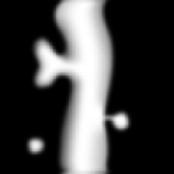
(a)	(b)	(c)
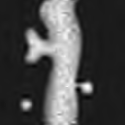
(d)	(e)	(f)
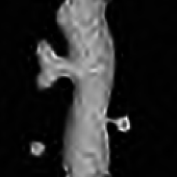
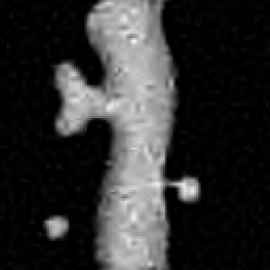
(g)	(h)

Fig. 1: Deconvolution of a simulated neuron (Intensity $\leqslant$ 30). (a) Original, (b) Blurred, (c) Blurred&noisy, (d) RL-TV, (e) NaiveGauss, (f) AnsGauss, (g) RL-MRS, (h) Our Algorithm.

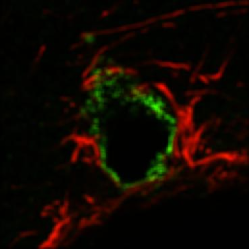
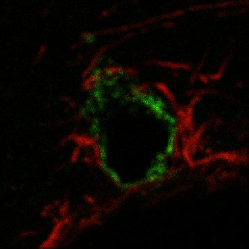
(a)	(b)	(c)
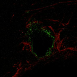
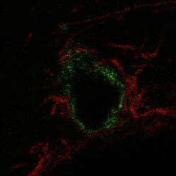
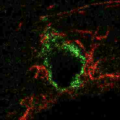
(d)	(e)	(f)
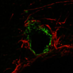
(g)	(h)

Fig. 2: Deconvolution of the cell image (Intensity $\leqslant$ 30). (a) Original, (b) Blurred, (c) Blurred&noisy, (d) RL-TV, (e) NaiveGauss, (f) AnsGauss, (g) RL-MRS, (h) Our Algorithm.

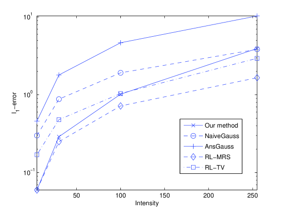
Fig. 3: Mean $\ell_{1}$-error of all algorithms as a function of the intensity level for the deconvolution of the cell

	Intensity regime
Method	$\leqslant 5$	$\leqslant 30$	$\leqslant 100$	$\leqslant 255$
Our method	0.21	0.76	2.39	4.79
NaiveGauss	0.41	0.89	2.31	5.15
AnsGauss	2.07	7.56	21.25	50.41
RL-MRS	0.21	0.96	2.2	4.51
RL-TV	0.73	1.47	2.72	4.28

Table 1: Mean $\ell_{1}$-error of all algorithms as a function of the intensity level for the deconvolution of the neuron phantom.

Method	Time (in s)
Our method	2.7
NaiveGauss	1.7
AnsGauss	1.7
RL-MRS	15
RL-TV	2.5

Table 2: Execution time for the simulated neuron using the orthogonal wavelet transform

6 Conclusion

In this paper, we presented a sparsity-based fast iterative thresholding deconvolution algorithm that take accounts of the presence of Poisson noise. Competitive results on confocal microscopy images with state-of-the-art algorithms are shown. The combination of several transforms leads to some advantages, as we can easily adapt the dictionary to the kind of image to restore. The parameter $\lambda$ can be tricky to find, and we are developing a method helping to solve this issue.

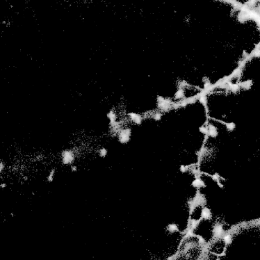
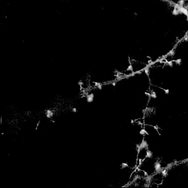
(a)	(b)

Fig. 4: Deconvolution of a real neuron. (a) Original noisy, (b) Restored with our algorithm

References

- [1] N. Dey et al., “A deconvolution method for confocal microscopy with total variation regularization,” in IEEE ISBI, 2004.
- [2] P. Sarder and A. Nehorai, “Deconvolution Method for 3-D Fluorescence Microscopy Images,” IEEE Sig. Pro., vol. 23, pp. 32–45, 2006.
- [3] J. Boutet de Monvel et al, “Image Restoration for Confocal Microscopy: Improving the Limits of Deconvolution, with Application of the Visualization of the Mammalian Hearing Organ,” Biophysical Journal, vol. 80, pp. 2455–2470, 2001.
- [4] C. Vonesch and M. Unser, “A fast iterative thresholding algorithm for wavelet-regularized deconvolution,” IEEE ISBI, 2007.
- [5] I. Daubechies, M. Defrise, and C. De Mol, “An iterative thresholding algorithm for linear inverse problems with a sparsity constraints,” CPAM, vol. 112, pp. 1413–1541, 2004.
- [6] P. L. Combettes and V. R. Wajs, “Signal recovery by proximal forward-backward splitting,” SIAM MMS, vol. 4, no. 4, pp. 1168–1200, 2005.
- [7] G. Teschke, “Multi-frame representations in linear inverse problems with mixed multi-constraints,” ACHA, vol. 22, no. 1, pp. 43–60, 2007.
- [8] C. Chaux, P. L. Combettes, J.-C. Pesquet, and V. R. Wajs, “A variational formulation for frame-based inverse problems,” Inv. Prob., vol. 23, pp. 1495–1518, 2007.
- [9] M. J. Fadili and J.-L. Starck, “Sparse representation-based image deconvolution by iterative thresholding,” in ADA IV, France, 2006, Elsevier.
- [10] C. Chaux, L. Blanc-Féraud, and J. Zerubia, “Wavelet-based restoration methods: application to 3d confocal microscopy images,” in SPIE Wavelets XII, 2007.
- [11] F-X Dupé, M.J. Fadili, and J.-L. Starck, “A proximal iteration for deconvolving poisson noisy images using sparse representations,” IEEE Trans. Im. Proc., 2008, submitted.
- [12] J.-L. Starck and F. Murtagh, Astronomical Image and Data Analysis, Springer, 2006.
- [13] B. Zhang, J. Zerubia, and J.-C. Olivo-Marin, “Gaussian approximations of fluorescence microscope PSF models,” OSA, 2006.