Abstract

We discuss ILC measurements for a specific MSSM scenario with CP phases, where the lightest neutralino is a good candidate for dark matter, annihilating efficiently through t-channel exchange of light staus. These prospective (CP-even) ILC measurements are then used to fit the underlying model parameters. A collider prediction of the relic density of the neutralino from this fit gives $0.116<\Omega h^{2}<0.19$ at 95% CL. CP-odd observables, while being a direct signal of CP violation, do not help in further constraining $\Omega h^{2}$. The interplay with (in)direct detection of dark matter and with measurements of electric dipole moments is also discussed. Finally we comment on collider measurements at higher energies for refining the prediction of $\Omega h^{2}$.

1 Introduction

One of the prime motivations for a high-energy and high-luminosity $e^{+}e^{-}$ linear collider is the possibility to do precision measurements of new particles beyond the Standard Model. The lightest of these new particles is often stable by virtue of a new discrete symmetry and hence a candidate for the dark matter (DM) of the Universe. One therefore hopes to be able to precisely determine the properties of the DM in the laboratory, and in particular to make a “collider prediction” of its relic abundance, which can be tested against cosmological models. For such a collider prediction to be of interest, it must be as precise as the value obtained from cosmological observations. This means a precision of about 10% (for 95% CL) to match WMAP+SDSS [1, 2, 3] or few percent to match expectations at the PLANCK satellite [4]. Moreover, if the annihilation cross section of the DM candidate is known, one can also predict direct and indirect DM detection cross sections as functions of astrophysical quantities such as galactic densities, see e.g. [5, 6].

The possibility to make collider predictions of the cross sections for annihilation of dark matter candidates has been examined within specific supersymmetric scenarios. Within the constrained minimal supersymmetric standard model (CMSSM), which has only a handful of free parameters, it has been shown in a case study [7] that the LHC could make a prediction for the DM relic density of the order of 10%, assuming the standard cosmological scenario; the ILC could reach a precision of few percent [8] in several scenarios. The particular case of stau co-annihilation in the CMSSM was investigated for the LHC in [9] and for the ILC in [10] with similar conclusions. In the general MSSM, it was shown that the LHC might match roughly the WMAP+SDSS precision in a favourable scenario [11] while the ILC could achieve much better precision [12]. These conclusions, however, depend very strongly on the scenario considered; many remain challenging for both the LHC and the ILC [12], see also [13]. Moreover, the studies mentioned here mainly concentrated on a few scenarios that provide the correct amount of neutralino annihilation, consistent with the WMAP+SDSS range. Furthermore –and more importantly– they assumed that CP is conserved, although CP-violating (CPV) phases are generic in the MSSM.

It is well known that CPV MSSM phases can have an important effect on the neutralino annihilation cross sections [14, 15, 16, 17, 18]. The consequences of phases for direct and indirect detection were examined in [15, 16, 19, 20, 21]. In [18], we performed a comprehensive analysis of the impact of CP phases on the relic density of neutralino dark matter, taking into account consistently phases in all (co-)annihilation channels, and carefully disentangling CPV effects due to modifications in the couplings from pure kinematic effects. We found variations in $\Omega h^{2}$ solely from modifications in the couplings of up to an order of magnitude. We concluded that the determination of the relevant couplings (including CPV phases!) can be as important for the prediction of $\Omega h^{2}$ as precision measurements of masses, i.e. pure sparticle spectroscopy.

In this paper, we therefore consider a particular scenario of the CPV MSSM, taken from [18], and investigate i) which measurements are possible at the ILC, ii) to which precision the underlying MSSM parameters and the neutralino relic density can be inferred from these measurements, and iii) what are the implications for direct and indirect DM detection and measurements of electric dipole moments (EDMs).

Our scenario has light gauginos and staus with masses below 200 GeV. The lightest supersymmetric particle (LSP) is the lightest neutralino with a mass of $\sim$80 GeV; it is dominantly bino. The two staus have masses of about 100 GeV and 180 GeV, with a strong mixing between the left- and right-chiral states. The neutralino LSP annihilates predominantly into tau pairs, with the annihilation cross section being sensitive to the stau mixing. Although the $\tilde{\tau}_{1}$ is very light, the scenario does not rely on coannihilation but on t-channel stau exchange. We therefore refer to it as the “stau-bulk” scenario. Such a scenario occurs in the CP-conserving MSSM only for $M_{1}<0$.

We further impose that the sfermions of the first and second generation are heavy in order to avoid the strong EDM constraints. The resulting mass pattern, light staus but TeV-scale selectrons and smuons, is not found in SUSY models where universality among scalar masses is imposed at a high scale. It is important to note that our scenario, despite having several particles below 200 GeV, is quite challenging for colliders. At the LHC, SUSY events are dominated by squark and gluino production followed by cascade decays leading to jets plus $\tau$’s plus $E_{T}^{\rm miss}$. At the ILC, two neutralinos, the lighter chargino, and the two staus are within kinematic reach with $\sqrt{s}=500$ GeV. However, production of these sparticles again only leads to taus plus missing energy.

The paper is organised as follows. Section 2 describes the detailed setup of our “stau-bulk” scenario. Expectations for ILC measurements are given in Section 3. In Section 4, we present our results concerning the determination of the model parameters and the prediction for the relic density of dark matter. In Section 5 we then discuss CP-sensitive observables, and in Section 6 additional possibilities to test and constrain the model at higher energies, through EDM measurements or through direct DM detection experiments. Finally, Section 7 contains our conclusions.

2 Setup of the stau-bulk scenario

In the MSSM, the parameters that can have CP phases are the gaugino and Higgsino mass parameters, $M_{i}=|M_{i}|e^{i\phi_{i}}$, with $i=1,2,3$, and $\mu=|\mu|e^{i\phi_{\mu}}$, and the trilinear sfermion-Higgs couplings, $A_{f}=|A_{f}|e^{i\phi_{f}}$. Not all of these phases are, however, physical. The physical combinations are Arg$(M_{i}\mu)$ and Arg$(A_{f}\mu)$. Allowing for CP-violating phases, in particular non-vanishing $\phi_{f}$, induces a mixing between the two CP-even states $h^{0}$, $H^{0}$ and the CP-odd state $A^{0}$. The resulting mass eigenstates $h_{1}$, $h_{2}$, $h_{3}$ ($m_{h_{1}}<m_{h_{2}}<m_{h_{3}}$) are no longer eigenstates of CP. Therefore the charged Higgs mass, $m_{H^{+}}$, is typically used as input parameter in the CPV-MSSM.

In this paper we investigate the “stau bulk” region of [18], which appears for light staus and large phase of $M_{1}$. The point is the following. In the conventional case, there are mainly two mechanisms that can make a light bino-LSP annihilate efficiently enough: resonant annihilation through the light Higgs, or co-annihilation with a sparticle that is close in mass –in the CMSSM typically the lighter stau. The so-called “bulk region” where the LSP annihilates through t-channel exchange of very light sleptons is largely excluded by LEP. For large phases of $M_{1}$ we have found, however, that the couplings of the neutralino to staus can be sufficiently enhanced such that a new region opens up, where the $\tilde{\chi}^{0}_{1}$–$\tilde{\tau}_{1}$ mass difference is too large for co-annihilation to be efficient but the LSP annihilates into taus through t-channel exchange of both $\tilde{\tau}_{1}$ and $\tilde{\tau}_{2}$.

To define a benchmark point for such a scenario, we choose the following input parameters at the electroweak scale:

$$\begin{array}[]{llll}M_{1}=80.47~{}{\rm GeV},&M_{2}=170.35~{}{\rm GeV},&M_{3}=700~{}{\rm GeV},&\phi_{1}=180^{\circ},\\ M_{\tilde{L}_{3}}=138.7~{}{\rm GeV},&M_{\tilde{E}_{3}}=135.2~{}{\rm GeV},&A_{\tau}=60~{}{\rm GeV},&\phi_{\tau}=0,\\ \mu=600~{}{\rm GeV},&\tan\beta=10,&\phi_{\mu}=0.\end{array}$$ (1)

All other parameters, i.e. sfermion masses, $A_{t,b}$, and $m_{H^{+}}$ are set to 1 TeV for simplicity. This way EDM constraints are avoided when varying $\phi_{1}$ and $A_{\tau}$; all other phases are assumed to vanish.

We use CPsuperH [22] to compute Higgs and sparticle masses and mixing angles, and micrOMEGAs 2.1 [23, 24] to compute the relic density, EDMs, and (in)direct detection cross sections. The mixing angle in the stau sector writes

$$\tan 2\,\theta_{\tilde{\tau}} = \frac{-2\,m_{\tau}\,(A_{\tau}-\mu\tan\beta)}{m^{2}_{\tilde{\tau}_{R}}-m^{2}_{\tilde{\tau}_{L}}}$$ (2)

and for our scenario is completely dominated by the $\mu\tan\beta$ term. The mass spectrum resulting from eq. (1) is given in Table 1. The particles accessible at ILC with $\sqrt{s}=500$ GeV are $\tilde{\chi}^{0}_{1}$, $\tilde{\chi}^{0}_{2}$, $\tilde{\chi}^{+}_{1}$, $\tilde{\tau}_{1}$, $\tilde{\tau}_{2}$ and $\tilde{\nu}_{\tau}$. Production cross sections and branching ratios are discussed in Section 3. At this stage we just note that the scenario is rather challenging to resolve experimentally because SUSY events involve only $\tau$’s and missing energy.

	$\tilde{\chi}^{0}_{1}$	$\tilde{\chi}^{0}_{2}$	$\tilde{\chi}^{0}_{3}$	$\tilde{\chi}^{0}_{4}$	$\tilde{\chi}^{+}_{1}$	$\tilde{\chi}^{+}_{2}$	$h_{1}$	$h_{2,3}$
	80.7	164.9	604.8	610.5	164.9	612.1	116.1	997.
	$\tilde{\tau}$	$\tilde{\nu}_{\tau}$	$\tilde{e}$	$\tilde{\nu}_{e}$	$\tilde{u}$	$\tilde{d}$	$\tilde{t}$	$\tilde{b}$
R(1)	100.9	–	1000.9	–	999.4	1000.3	939.1	995.6
L(2)	177.2	123.1	1001.1	998.0	998.6	1001.7	1075.6	1006.4

Table 1: Masses of particles for the input parameters of eq. (1).

The relic density of the $\tilde{\chi}^{0}_{1}$ is $\Omega h^{2}=0.130$ at the nominal point eq. (1). As mentioned above, the dominant annihilation channel is into tau pairs (more than 95% of the total contribution) through t-channel exchange of staus. The contribution of both $\tilde{\tau}_{1}$ and $\tilde{\tau}_{2}$ is crucial in bringing $\Omega h^{2}$ to the desired range, $0.094<\Omega h^{2}<0.136$ [25]. Indeed, for $\phi_{1}=0$ (or $M_{1}$ positive) one would have $\Omega h^{2}=0.167$. Note also that the mass splitting between the stau-NLSP and the LSP is too large for any significant contribution from co-annihilation.

The precision with which $\Omega h^{2}$ can be inferred from ILC measurements therefore depends not only on the accuracy of the sparticle spectroscopy (mass measurements) but on the determination of all parameters of the neutralino sector ($M_{1}$, $M_{2}$, $\mu$, $\tan\beta$, $\phi_{1}$), which determine the LSP mass and couplings, and the four parameters of the stau sector ($M_{\tilde{\tau}_{L}}$, $M_{\tilde{\tau}_{R}}$, $A_{\tau}$, $\phi_{\tau}$). The dependence on $\phi_{1}$, and to a much lesser extent $\phi_{\tau}$, originates from the $\tilde{\chi}^{0}_{1}\tilde{\tau}_{1,2}\tau$ couplings. In addition, particles which are too heavy to be produced at ILC could have some influence. Indeed, the exclusion of selectrons and smuons up the the kinematic limit, $m_{\tilde{l}}>250$ GeV, leaves an uncertainty in $\Omega h^{2}$ of about 7%. The influence of heavy Higgs states gives $\delta\Omega/\Omega\simeq 5\%$ for $m_{h_{2,3}}\simeq 250$ GeV. The combined effect from sleptons and Higgses is actually smaller, because their contributions work against each other, so we have $\delta\Omega/\Omega\simeq 7\%$ as overall uncertainty from the unknown part of the spectrum. The dependence on $m_{\tilde{e},\tilde{\mu}}$ and $m_{h_{2,3}}$ is illustrated in Fig. 1.

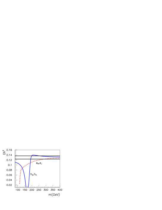
Figure 1: Dependence of $\Omega h^{2}$ on $m_{\tilde{e},\tilde{\mu}}$ (dashed red line) and $m_{h_{2,3}}$ (full blue line) for the nominal point eq. (1). The horizontal lines indicate $\delta\Omega/\Omega=\pm 5\%$.

We assume here that the mass scale of the squarks and gluino is known from LHC. The LHC can also provide additional information on the heavy Higgs states: a charged Higgs with mass up to $m_{H^{+}}\simeq 500$ GeV could be discovered/excluded at the LHC in the channel $gb\to H^{-}t$ with $H^{-}\to\tau\nu$ for $\tan\beta=10$[26]. If the neutral heavy Higgses weigh more than $250$ GeV, the LHC has limited discovery potential using SM decay modes at intermediate values of $\tan\beta$. However, a recent analysis [27] has shown how to exploit the Higgs into chargino/neutralino decay modes into four leptons (electrons or muons) in this region. Although no dedicated analysis has been performed for decays into taus, a similar coverage as in [27] can be expected in our scenario [28].

3 ILC measurements

3.1 Event generation and analysis

The analysis presented in this section assumes a detector as described in the Tesla TDR [29]. The simulations are based on Simdet 4.02 [30] with an acceptance $\theta>125$ mrad and $e,\,\gamma$ veto of $\theta>4.6$ mrad. Background and signal events are generated with Pythia 6.2 [31] including beam polarisations $({\cal P}_{e^{-}},{\cal P}_{e^{+}})=(0.8,0.6)$, QED radiation and beamstrahlung à la Circe [32]. $\tau$ decays and polarisation are treated with Tauola [33]. The SM background includes $e^{+}e^{-}\to W^{+}W^{-}$ and the negligible pair production $e^{+}e^{-}\to\tau^{+}\tau^{-}(\gamma)$. The $\gamma\gamma$ background is also negligible with $\sigma(e^{+}e^{-}\to e^{+}e^{-}\tau^{+}\tau^{-})=4.5\cdot 10^{5}~{}\mathrm{fb}$ and an acceptance $<{\rm few}10^{-6}$.

To measure the particle masses, two methods are available: threshold scans and endpoint methods. Both will be useful in our case. In slepton decays to LSP, ${\tilde{\ell}}^{-}\to\ell^{-}\,\tilde{\chi}^{0}_{1}$, the endpoints, i.e. maxima and minima $E_{+/-}$ in the flat lepton energy spectra:

$$E_{+/-} = \frac{\sqrt{s}}{4}\left(1-\frac{m_{\tilde{\chi}}^{2}}{m_{{\tilde{\ell}}}^{2}}\right)\,(1\pm\beta)\;,$$ (3)

where $\beta=\sqrt{1-4m_{{\tilde{\ell}}}^{2}/s}$, can be used to extract the slepton and neutralino mass.

The mixing angle in the stau sector, eq. (2), can either be determined from measurements of the polarized cross section or from the measurement of the $\tau$ polarisation ${\cal P}_{\tau}$ in the decay ${\tilde{\tau}}_{1}\to\tau\tilde{\chi}^{0}_{1}$ [34, 35, 36]. Note that ${\cal P}_{\tau}$ depends not only on the mixing anlge $\theta_{\tilde{\tau}}$ of the staus but also on the mixing of the lightest neutralino.

The selection criteria used in $e^{+}e^{-}\to{\tilde{\tau}}^{+}_{1}{\tilde{\tau}}^{-}_{1}\to\tau^{+}\tau^{-}E^{\rm miss}$ are essentially to require two acoplanar $\tau$ jets ($\Delta\phi<180^{\circ}$ and $m_{\tau}<2\;\mathrm{GeV}$) being produced centrally ($|\!\cos\theta|<0.75$). In addition, topology dependent $p_{\perp}$ cuts are applied to reject $\gamma\gamma$ reactions [10]. The overall efficiency for ${\tilde{\tau}}_{1}$-pair reconstruction is $\epsilon\simeq 0.32$ at $\sqrt{s}=280\;\mathrm{GeV}$ and varies only slowly with the cms energy. The same selection criteria are applied to detect the other sparticle decays during an energy scan.

Despite the large statistics, the leptonic $\tau$ decays are not useful due to the large $WW$ background. We therefore only analyse the decay modes $\tau\to\pi\nu_{\tau},\;\rho\nu_{\tau},\;3\pi\nu_{\tau}$ with branching ratios ${\cal B}(\tau\to\pi\nu_{\tau})=0.111,\ {\cal B}(\tau\to\rho\nu_{\tau})=0.254,\ {\cal B}(\tau\to 3\pi\nu_{\tau})=0.194$.

3.2 Masses from threshold scan

At $\sqrt{s}=500\;\mathrm{GeV}$, all SUSY signals are completely dominated by the $\tau\tau E^{\rm miss}$  topology. The challenge is then to disentangle the various sources. The strategy we propose is to scan downwards in energy in steps of 10 GeV in order to find thresholds. This is done using different beam polarisations $e^{-}_{R}e^{+}_{L}$ [$\sigma_{RL}$] and $e^{-}_{L}e^{+}_{R}$ [$\sigma_{LR}$] where ${\cal P}_{e-}=\pm 0.8$ and ${\cal P}_{e^{+}}=\mp 0.6$. The ${\tilde{\tau}}_{i}^{+}{\tilde{\tau}}_{j}^{-}$ pair production is best detected in the $\sigma_{RL}$ polarisation mode, while $\sigma_{LR}$ is dominated by $\tilde{\chi}^{+}_{1}\tilde{\chi}^{-}_{1}$ production The results of a scan of the visible cross sections $e^{+}e^{-}\to\tau\tau E^{\rm miss}$  are shown in Fig. 2. Clearly, integrated luminosities of $2\;\mathrm{fb}^{-1}$ per step in energy are sufficient. Fitting the excitation curves, $\sigma_{{\tilde{\tau}}{\tilde{\tau}}}\sim\beta^{3}$ of Fig. 2a and $\sigma_{\tilde{\chi}^{+}\tilde{\chi}^{-}}\sim\beta$ of Fig. 2b, allows a determination of the sparticle masses. Note that the mixed ${\tilde{\tau}}_{1}{\tilde{\tau}}_{2}$ production is hardly detectable and can only be accomodated in a global fit including all channels. The results of a fit for ${\tilde{\tau}}_{1}$, $\tilde{\chi}^{+}_{1}$ and ${\tilde{\tau}}_{2}$ masses together with the total integrated luminosity used in each case are listed in Table 2. The expected accuracies can easily be scaled with the luminosity.

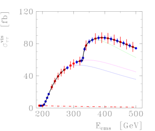
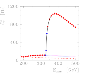
Figure 2: Visible cross section as a function of cms energy of the inclusive reaction $e^{+}_{L}e^{-}_{R}\to\tau^{+}\tau^{-}\,E^{\rm miss}$ (left) and $e^{+}_{R}e^{-}_{L}\to\tau^{+}\tau^{-}\,E^{\rm miss}$ (right). The red (blue) points correspond to integrated luminosities of ${\cal L}=2\,\mathrm{fb}^{-1}(10\,\mathrm{fb}^{-1})$, the contributions of $W^{+}W^{-}$ (dash-dot), ${\tilde{\tau}}_{1}^{+}{\tilde{\tau}}_{1}^{-}$ (blue), ${\tilde{\tau}}_{1}^{\pm}{\tilde{\tau}}_{2}^{\mp}$ (pink), $\tilde{\chi}^{+}_{1}\tilde{\chi}^{-}_{1}$(green) and ${\tilde{\tau}}_{2}^{+}{\tilde{\tau}}_{2}^{-}$ are indicated.

reaction	$m~{}[\mathrm{GeV}]$	${\cal L}~{}[\mathrm{fb}^{-1}]$
$e^{+}_{L}e^{-}_{R}\to{\tilde{\tau}}_{1}{\tilde{\tau}}_{1}$	$100.92\pm 0.40$	$50$
$e^{+}_{R}e^{-}_{L}\to\tilde{\chi}^{+}_{1}\tilde{\chi}^{-}_{1}$	$164.88\pm 0.015$	$30$
$e^{+}_{L}e^{-}_{R}\to{\tilde{\tau}}_{2}{\tilde{\tau}}_{2}$	$188.2\pm 9.1$	$100$

Table 2: Results of mass fits from the excitation curves indicating the reactions, beam polarisation and assumed integrated luminosity

3.3 LSP mass from stau decays

An alternative method for measuring the ${\tilde{\tau}}_{1}$ mass and/or the $\tilde{\chi}^{0}_{1}$ LSP mass is to use the energy spectra in ${\tilde{\tau}}_{1}\to\tau\tilde{\chi}^{0}_{1}$ decays. However, the $\tau$ energy spectrum reconstructed from the $\tau$ decay products is no longer flat due to undetected neutrinos, and the extraction of the endpoint energies, see eq. (3), gets more involved [35, 36]. The upper endpoint energy $E_{+}$ can be identified with the maximum energy of the decay products and can still be determined rather well. The lower endpoint energy $E_{-}$ is in general completely distorted. It may be reconstructed from the pion energy $E_{\pi}$ spectrum of $\tau\to\pi\;\nu_{\tau}$, but the expected precision is poor due the low branching ratio and a polarisation ${\cal P}_{\tau}$ dependent shape of the energy distribution. Therefore, determining both stau and neutralino masses from the energy spectra alone is not very meaningful and we use the additional information on $m_{{\tilde{\tau}}_{1}}$ from the threshold scan.

In order to study the properties of stau decay spectra, the maximal energy for ${\tilde{\tau}}_{1}^{+}{\tilde{\tau}}_{1}^{-}$ production at $\sqrt{s}=280\;\mathrm{GeV}$ just below the threshold for other sparticles is chosen. A fit to the $E_{\pi}$ spectrum (not shown) yields $E_{-}=7.8\pm 0.50\;\mathrm{GeV}$ and $E_{+}=42.8\pm 0.30\;\mathrm{GeV}$. In $\tau\to\rho\;\nu_{\tau}\to\pi^{\pm}\pi^{0}\;\nu_{\tau}$ and $\tau\to 3\pi\;\nu_{\tau}\to\pi^{\pm}\pi^{\pm}\pi^{\mp}\;\nu_{\tau}+\pi^{\pm}\pi^{0}\pi^{0}\;\nu_{\tau}$ the energies $E_{\rho}$ and $E_{3\pi}$ have the advantage of being independent of ${\cal P}_{\tau}$. The analysis of $E_{jet}\ (=E_{\rho}+E_{3\pi})$ spectrum is shown in Fig. 3, a fit to the energy distribution using an analytic formula gives the upper endpoint $E_{+}=42.8\pm 0.20\;\mathrm{GeV}$. Applying eq. (3) together with the results from the excitation curve leads to a LSP mass of $m_{\tilde{\chi}^{0}_{1}}=80.67\pm 0.35\;\mathrm{GeV}$ and a stau mass of $m_{{\tilde{\tau}}_{1}}=100.92\pm 0.39\;\mathrm{GeV}$. The $m_{\tilde{\chi}^{0}_{1}}-m_{{\tilde{\tau}}_{1}}$ correlation is shown in Fig. 3. Obviously an improved accuracy on $m_{{\tilde{\tau}}_{1}}$ will result in a smaller error on the LSP mass.

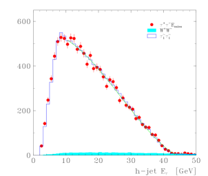
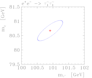
Figure 3: Energy spectrum $E_{jet}$ from $\tau\to\rho\;\nu_{\tau}+3\pi\;\nu_{\tau}$ of the reaction $e^{+}_{L}e^{-}_{R}\to{\tilde{\tau}}^{+}_{1}{\tilde{\tau}}^{-}_{1}$ including background from $W^{+}W^{-}\to\tau^{+}\tau^{-}\;E_{miss}$; the data points represent a simulation assuming ${\cal L}=200\,\mathrm{fb}^{-1}$ at $\sqrt{s}=280\,\mathrm{GeV}$, the blue histogram corresponds to a very high statistics sample, the green curve is a fit to an analytic formula (left). Correlation $m_{\tilde{\chi}^{0}_{1}}$ vs $m_{{\tilde{\tau}}_{1}}$ using the stau mass from the excitation curve and the end point energy from the $E_{jet}$ spectrum (right).

3.4 Stau mixing angle

The stau mixing angle can be determined from measurements of polarized cross sections. Again, the energy for ${\tilde{\tau}}_{1}$ pair production is chosen below the threshold for other sparticles production, that is $\sqrt{s}=280$ GeV. At this energy we expect $\sigma_{RL}=155.5\pm 2.2\,\mathrm{fb}$ where the error corresponds to an integrated luminosity of ${\cal L}=200\,\mathrm{fb}^{-1}$ and includes an estimate of systematics from acceptance calculations, branching ratios and $WW$ background subtraction; for comparison see the visible cross section in Fig. 2.

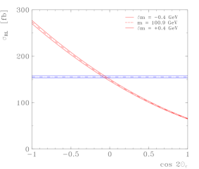
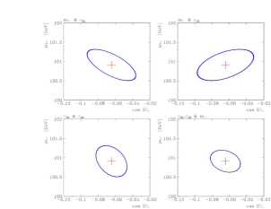
Figure 4: Dependence of ${\tilde{\tau}}_{1}{\tilde{\tau}}_{1}$ polarised cross section $\sigma_{RL}$ on the ${\tilde{\tau}}$ mixing angle $\cos 2\theta_{\tilde{\tau}}$ at $\sqrt{s}=280\,\mathrm{GeV}$, the blue band indicates a measurement assuming ${\cal L}=200\,\mathrm{fb}^{-1}$ (left): correlation $m_{{\tilde{\tau}}_{1}}$ vs $\cos 2\theta_{\tilde{\tau}}$ using the stau mass from the excitaion curve the cross section $\sigma_{RL}$ (right).

The polarised cross section $\sigma_{RL}$ dependence on the mixing angle $\cos 2\theta_{\tilde{\tau}}$ [36] is shown in Fig. 4. Fitting both the mixing angle $\cos 2\theta_{\tilde{\tau}}$ and the mass $m_{\tilde{\tau}_{1}}$ to the cross sections in the continuum and at threshold yields $\cos 2\theta_{\tilde{\tau}}=-0.065\pm 0.028$ and $m_{{\tilde{\tau}}_{1}}=100.92\pm 0.40\;\mathrm{GeV}$. The $m_{{\tilde{\tau}}_{1}}$–$\cos 2\theta_{\tilde{\tau}}$ correlation contour is shown in Fig. 4. The accuracy can be improved by adding another cross section measurement with different polarisation, e.g. $\sigma_{LR}=157.3\pm 3.5\,\mathrm{fb}$ assuming ${\cal L}=200\,\mathrm{fb}^{-1}$. Using all observables, $\sigma_{RL}$, $\sigma_{LR}$ and $m_{{\tilde{\tau}}_{1}}(\sigma_{thr})$, one expects a precision of $\delta m_{{\tilde{\tau}}_{1}}=0.35\;\mathrm{GeV}$ and $\delta\!\cos 2\theta_{\tilde{\tau}}=0.017$.

3.5 Tau polarisation

The polarisation ${\cal P}_{\tau}$ of the tau stemming from the ${\tilde{\tau}}_{i}\to\tau\tilde{\chi}^{0}_{1}$ decay gives additional information on the stau and neutralino mixings [34]. Since $\cos 2\theta_{\tilde{\tau}}$ is obtained from polarized cross sections as explained above, ${\cal P}_{\tau}$ is in particular useful to constrain the gaugino–higgsino composition of the LSP. Here, we exploit the decay $\tau\to\rho\nu_{\tau}\to\pi\pi^{0}\nu_{\tau}$. The ratio $z_{\pi}=E_{\pi}/E_{\rho}$ is indeed sensitive to ${\cal P}_{\tau}$ and independent of $m_{{\tilde{\tau}}_{1}}$. For a right-handed $\tau$ (${\cal P}_{\tau}=+1$), the $\rho$ is longitudinally polarized and the distribution ${\rm d}\sigma/{\mathrm{d}}z_{\pi}\propto(2z_{\pi}-1)^{2}$ is peaked near $z_{\pi}\to 0{\rm~{}or~{}}1$, while for a left-handed $\tau$ (${\cal P}_{\tau}=-1$), the $\rho$ is transversely polarized and the distribution ${\rm d}\sigma/{\rm d}z_{\pi}\propto 2z_{\pi}(1-z_{\pi})$ is peaked at $z_{\pi}=0.5$. The analysis of the $z_{\pi}$ spectrum is shown in Fig. 5. The results of a fit to the ${\tilde{\tau}}_{1}$ polarisation leads to ${\cal P}_{\tau}=0.64\pm 0.035$ for an input value ${\cal P}_{\tau}=0.641$.

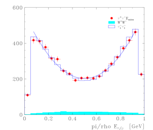
Figure 5: Energy spectrum $z_{\pi}=E_{\pi}/E_{\rho}$ from $\tau\to\rho\;\nu_{\tau}\to\pi\pi^{0}\;\nu_{\tau}$ of the reaction $e^{+}_{L}e^{-}_{R}\to{\tilde{\tau}}^{+}_{1}{\tilde{\tau}}^{-}_{1}$ including background from $W^{+}W^{-}\to\tau^{+}\nu\;\tau^{-}\nu$. The data points represent a simulation assuming ${\cal L}=200\,\mathrm{fb}^{-1}$ at $\sqrt{s}=280\,\mathrm{GeV}$, the blue histogram corresponds to a very high statistics sample, the blue curve is a fit to the data with a ${\tilde{\tau}}_{1}$ polarisation ${\cal P}_{\tau}=0.64\pm 0.035$.

In summary, simulations of stau production $e^{+}e^{-}\to{\tilde{\tau}}_{i}{\tilde{\tau}}_{j}$ and chargino production $e^{+}e^{-}\to\tilde{\chi}^{+}_{1}\tilde{\chi}^{-}_{1}$ under realistic experimental conditions assuming $({\cal P}_{e^{-}},{\cal P}_{e^{+}})=(0.8,0.6)$ show that the stau, neutralino and chargino masses as well as the polarisation ${\cal P}_{{\tilde{\tau}}_{1}\to\tau\tilde{\chi}^{0}_{1}}$ and mixing parameter $\theta_{\tilde{\tau}}$ can be accurately determined with moderate integrated luminosity. The possible ILC measurements are summarized in Table 3.

channel	observables
${\tilde{\tau}}_{1}^{+}{\tilde{\tau}}_{1}^{-}$	$m_{{\tilde{\tau}}_{1}}=100.92\pm 0.40~{}\mathrm{GeV}$   $m_{\tilde{\chi}^{0}_{1}}=80.67\pm 0.35~{}\mathrm{GeV}$
	$\cos 2\,\theta_{\tilde{\tau}}=-0.065\pm 0.028$   ${\cal P}_{\tau}=0.64\pm 0.035$
${\tilde{\tau}}_{2}^{+}{\tilde{\tau}}_{2}^{-}$	$m_{{\tilde{\tau}}_{2}}=176.9\pm 9.1~{}\mathrm{GeV}$
$\tilde{\chi}^{+}_{1}\tilde{\chi}^{-}_{1}$	$m_{\tilde{\chi}^{\pm}_{1}}=164.88\pm 0.015~{}\mathrm{GeV}$

Table 3: Summary of achievable precisions of ILC measurements.

4 DM properties: fit to ILC observables

Having established how precisely one could measure various CP-even observables at ILC, we now estimate how this would constrain the parameters of the underlying model, and the properties of the dark matter candidate. To this aim we perform a fit to the six observables listed in Table 3 assuming Gaussian errors. We also compute the total $\tau\tau$ SUSY cross section at $\sqrt{s}=400$ GeV with polarized beams and add it to the fit: $\sigma(\tau\tau)=3.220\pm 0.046$ pb (for 10 fb^-1). Here we assume a systematic error as large as the statistical error. As free parameters we take

$$M_{1},\quad\mu,\quad\tan\beta,\quad M_{\tilde{L}_{3}},\quad M_{\tilde{R}_{3}},\quad A_{\tau},\quad\phi_{1},\quad\phi_{\tau}\,.$$ (4)

Owing to the extremely small experimental error on $m_{\tilde{\chi}^{\pm}_{1}}$, we do not include $M_{2}$ as an independent variable in the fit but compute it from $\mu$ and $\tan\beta$ such that it matches the measured value of $m_{\tilde{\chi}^{\pm}_{1}}$. The other SUSY parameters are fixed to the values specified in Sect. 2. We do not include the light Higgs mass in the fit because of the large parametric uncertainty from not knowing the parameters of the stop sector. This will be discussed in more detail after having summarized our main results.

To probe efficiently the multidimensional parameter space, we perform a Markov Chain [37] Monte Carlo (MCMC) analysis using a Metropolis-Hastings algorithm [38, 39, 40]. This algorithm generates a candidate state $x^{c}$ from the present state $x^{t}$ using a proposal density $Q(x^{t};x^{c})$. The candidate state is accepted to be the next state $x^{t+1}$ in the chain if

$$p=\frac{P(x^{c})Q(x^{t};x^{c})}{P(x^{t})Q(x^{c};x^{t})}\,,$$ (5)

where $P(x)$ is the probability calculated for the state $x$, is greater then a uniform random number $a=U(0,1)$. If the candidate is not accepted, the present state $x^{t}$ is retained and a new candidate state is generated. For the proposal density, we use a Gaussian distribution that is centered at $x^{t}$ and has a width $\sigma$ for each parameter of eq. (4). Moreover, we assume flat priors and take $P(x)=e^{-\chi^{2}(x)/2}$. A parameter point is hence accepted in the Markov Chain, $x^{t+1}=x^{c}$, if

$$p=e^{(\chi^{2}(x^{t})-\chi^{2}(x^{c}))/2}>U(0,1).$$ (6)

The $\chi^{2}$ function is computed as

$$\chi^{2}(x)=\sum_{i}\frac{X_{i}(x)-\overline{X}_{i}}{\sigma(\overline{X}_{i})}$$ (7)

where $\overline{X}_{i}$ and $\sigma(\overline{X}_{i})$ are the nominal values of the observables and their 1-$\sigma$ errors, and $X_{i}(x)$ are the corresponding values obtained at the parameter point $x$. Note that, including the $\tau\tau$ cross section, we have seven measurements ($i=1,...,7$) and eight free parameters, cf. eq. (4).

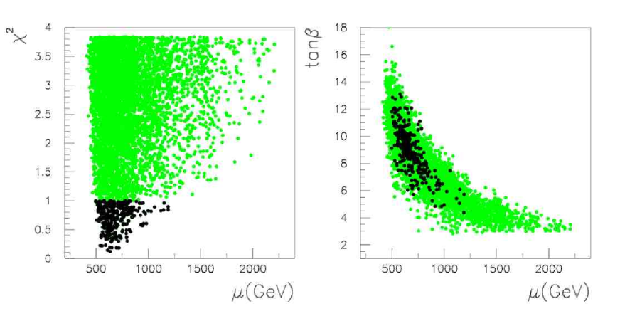
Figure 6: Results of the MCMC fit; in (a) $\chi^{2}$ as a function of $\mu$, in (b) the $1\sigma$ (black) and $2\sigma$ (green) allowed regions projected onto the $\mu$ versus $\tan\beta$ plane.

We run $5\times 10^{5}$ points on 10 independent chains, with the starting points having very different characteristics, such as large or small $\mu$; or $M_{\tilde{L}_{3}}$ smaller, larger, or equal $M_{\tilde{R}_{3}}$. We also include two randomly chosen starting points, for which we run $10^{6}$ points. While some of the chains start off with huge $\chi^{2}$’s, they all converge fast to $\chi^{2}\sim{\cal O}(1)$. We do not only keep the points accepted in the chains but also write out to a separate file all points tried which have $\chi^{2}<3.84$, corresponding to $95\%$ CL. Figure 6a shows the $\chi^{2}$ distribution of these points as a function of $\mu$. It has a minimum around $\mu\sim 600$ GeV, rises rather steeply for lower values and only slowly for higher values of $\mu$. We can gather from this plot that $\mu$ is determined only to $500~{}{\rm GeV}\;\raisebox{-3.87495pt}{$\textstyle\stackrel{{\scriptstyle\textstyle<}}{{\sim}}$}\;\mu\;\raisebox{-3.87495pt}{$\textstyle\stackrel{{\scriptstyle\textstyle<}}{{\sim}}$}\;1200~{}{\rm GeV}$ at $1\sigma$ from the ILC measurements. The reason is a kind of ‘valley’ of $\chi^{2}$ minima in the $\tan\beta$–$\mu$ plane. This is illustrated in Fig. 6b which shows in green (black) points which fall within the $2\sigma$ ($1\sigma$) region in the plane of $\tan\beta$ versus $\mu$. As can be seen, while $\tan\beta$ and $\mu$ are not very much constrained by the ILC measurements, there is a strong correlation between the two parameters. Projections of the $1\sigma$ and $2\sigma$ fitted regions onto the other parameters are shown in Fig. 7. The fit results at 95% CL can be summarized as follows.

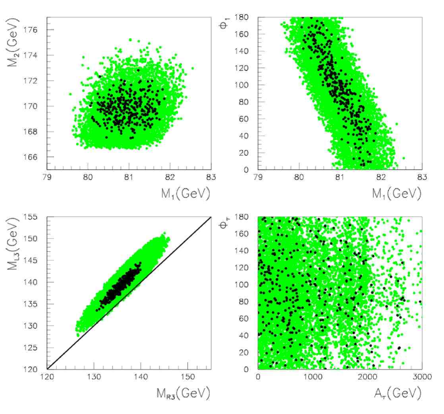
Figure 7: The $1\sigma$ (black) and $2\sigma$ (green) allowed regions projected in different planes: (a) $M_{1}$ vs. $M_{2}$, (b) $M_{1}$ vs. $\phi_{1}$, (c) $M_{\tilde{R}_{3}}$ vs. $M_{\tilde{L}_{3}}$ and (d) $A_{\tau}$ vs. $\phi_{\tau}$.

• The lack of observables individually sensitive to $\mu$ and $\tan\beta$ leaves a large allowed parameter space with $400<\mu<2200$ and $2.8<\tan\beta<18$. Note, however, that because the stau mixing is proportional to $(A_{\tau}-\mu\tan\beta)$ and because in general $\mu\tan\beta\gg A_{\tau}$ these two parameters are strongly correlated.

• The very precise determination of $m_{\tilde{\chi}^{0}_{1}}$ and $m_{\tilde{\chi}^{+}_{1}}$ constrains $M_{1}$ and $M_{2}$ to $\delta M_{1}=-0.9,\,+2.1$ GeV and $\delta M_{2}=-3.7,\,+4.9$ GeV.

• Although the phase $\phi_{1}$ can take any value, there is a correlation with the value of $M_{1}$: a large phase is associated with lower values of $M_{1}$. This is a direct consequence of the precise measurement of the neutralino mass.

• The measurement of the masses of both staus and their mixing angle well constrain $M_{\tilde{L}_{3}}$ and $M_{\tilde{R}_{3}}$ to about 10 GeV. Moreover, solutions with $M_{\tilde{L}_{3}}<M_{\tilde{R}_{3}}$ are strongly disfavoured.

• The trilinear coupling $A_{\tau}$ is basically undetermined, and the phase is $\phi_{\tau}$ completely unconstrained. This is because the stau mixing is dominated by the term $\mu\tan\beta$. The few points at low $\tan\beta\sim 4$ and $\mu\;\raisebox{-3.87495pt}{$\textstyle\stackrel{{\scriptstyle\textstyle<}}{{\sim}}$}\;1$ TeV in Fig. 6b have very large $|A_{\tau}|\;\raisebox{-3.87495pt}{$\textstyle\stackrel{{\scriptstyle\textstyle<}}{{\sim}}$}\;3$ TeV. Setting an upper limit on $|A_{\tau}|$ somewhat tightens the lower border of the $2\sigma$ $\tan\beta$–$\mu$ range in Fig. 6b.

Having determined the allowed parameter space, we next show in Fig. 8 the predictions for the relic density of dark matter. The allowed range at $2\sigma$ is found to be $0.116<\Omega h^{2}<0.19$. As expected, $\Omega h^{2}$ tends to be larger than the range that best fits present cosmological data. The lowest values of $\Omega h^{2}$ are obtained for a large phase $\phi_{1}$ and both $m_{\tilde{\tau}_{L}}$ and $m_{\tilde{\tau}_{R}}$ near their maximal allowed value. While there is no strong correlation between $\mu$ and $\Omega h^{2}$, see Fig. 8(a), it is only for $\mu\approx 500$–$700$ GeV that $\Omega h^{2}\;\raisebox{-3.87495pt}{$\textstyle\stackrel{{\scriptstyle\textstyle>}}{{\sim}}$}\;0.18$. This is because for small $\mu$ an increased higgsino component (although the LSP is always dominantly bino) leads to a smaller annihilation cross section into tau pairs. Furthermore, the mass of the LSP is too small for this to be compensated by the very efficient annihilation of the higgsino component into W pairs.

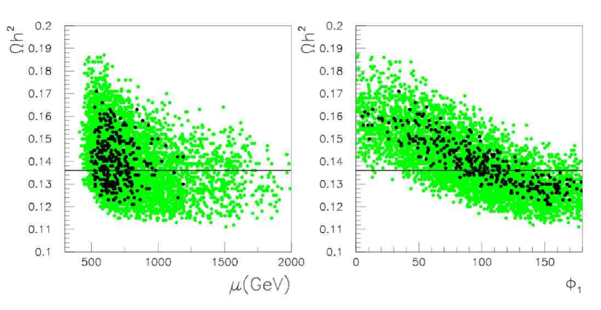
Figure 8: Predictions for (a) $\Omega h^{2}$ vs. $\mu$ and (b) $\Omega h^{2}$ vs. $\phi_{1}$ in the $1\sigma$ (black) and $2\sigma$ (green) fitted regions. Straight lines show $2\sigma$ upper limits on $\Omega h^{2}=0.136$

As mentioned above we do not include the light Higgs mass in our fit. This may seem surprising since $m_{h}$ can be measured very precisely at the ILC. Moreover, it strongly depends on $\tan\beta$ and might therefore be used to determine $\tan\beta$ and, in turn, constrain $\mu$. However, one must not forget that $m_{h}$ also strongly depends on the parameters of the stop sector. Indeed, if the stop parameters are not known, this induces a parametric uncertainty of about 15 GeV in $m_{h}$. As a consequence, the very precise measurement of $m_{h}$ expected at the ILC only poorly constrains $\tan\beta$ if the stop sector is not measured well. For illustration, Fig. 9(a) shows the correlation between $m_{h}$ and $\tan\beta$ in the $2\sigma$ fitted region for stop parameters fixed to their nominal values. Figure 9(b) shows the same but assuming that the stop masses are known to 10% (blue points) or that the stop sector is basically unknown (green points). Here note that in our scenario even the discovery of the stops is supposed to be very difficult at the LHC because of the overwhelming $t\bar{t}$ background. A measurement of $m_{h}=116.1$ GeV and stop masses known to 10% accuracy would constrain $\tan\beta$ only to about 3–14, theoretical uncertainties not included. In turn, since in our fit the stop parameters are fixed to 1 TeV, we allow Higgs masses as low as 100 GeV, because one can always find a combination of $m_{\tilde{t}_{1}}$, $m_{\tilde{t}_{2}}$ and $A_{t}$ which lifts $m_{h}$ above the LEP limit.

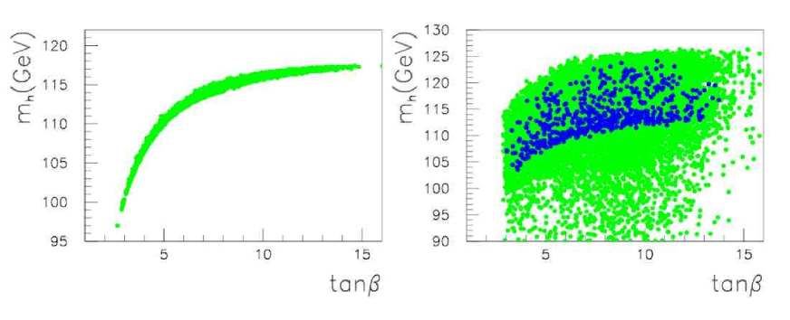
Figure 9: The $2\sigma$ region for $m_{h}$ as a function of $\tan\beta$: in (a) for parameters of the stop fixed to their nominal values and in (b) for varying stop parameters. In (b), the green points show the situation for a completely undetermined stop sector while the blue points are for stop masses known to $\pm 10\%$.

5 CP-odd observables

In the previous sections, we have demonstrated how the parameters $M_{1}$, $M_{2}$, $\mu$, etc, of our stau-bulk scenario can be determined or at least constrained from an analysis of particle masses, cross sections, distributions at the ILC. Being CP even, such quantities principally allow to determine CPV phases only up to a twofold ambiguity, $\phi\leftrightarrow 2\pi-\phi$. In our scenario, only a correlation between $M_{1}$ and $\phi_{1}$ can be obtained, c.f. Fig. 7(b). In order to test for non-trivial phases, one needs CP-odd observables. These could be T-odd observables based on triple-products in the production and decay of neutralinos or charginos, which are kinematically accessible in our scenario, $e^{+}e^{-}\to\tilde{\chi}_{1}^{0}\tilde{\chi}_{2}^{0}$ and $e^{+}e^{-}\to\tilde{\chi}_{1}^{+}\tilde{\chi}_{1}^{-}$, respectively.

5.1 Neutralino production and decay

For the cross section $\sigma$ of neutralino production, $e^{+}e^{-}\to\tilde{\chi}_{1}^{0}\tilde{\chi}_{2}^{0}$, followed by the subsequent two-body decay chain $\tilde{\chi}_{2}^{0}\to\tilde{\tau}_{1}^{\pm}\tau^{\mp}$, $\tilde{\tau}_{1}^{\pm}\to\tilde{\chi}_{1}^{0}\tau^{\pm}$, we define the T-odd asymmetry [41, 42, 43]

$$A_{1}=\frac{\sigma({\mathcal{T}}>0)-\sigma({\mathcal{T}}<0)}{\sigma({\mathcal{T}}>0)+\sigma({\mathcal{T}}<0)},$$ (8)

of the triple product

$${\mathcal{T}} = ({\bf p}_{e^{-}}\times{\bf p}_{\tau^{-}})\cdot{\bf p}_{\tau^{+}},$$ (9)

of the three-momenta ${\bf p}$. In Figure 10(a), we show the triple-product asymmetry $A_{1}$ as a function of $\phi_{1}$ in the $1\sigma$ and $2\sigma$ fitted regions. As can be seen, a measurement of $A_{1}\not=0$ would be a very clear signal of CP violation. Unfortunately, this does not help constrain $\Omega h^{2}$ due to the two-fold ambiguity in $\phi_{1}$, see Fig. 10(b). Note also that in our scenario, the neutralino production cross sections are suppressed due to the heavy selectron masses $m_{\tilde{e}_{L,R}}=1$ TeV, however can be as large as $10$ fb for $(P_{e^{-}},P_{e^{+}})=(0.8,-0.6)$ at $\sqrt{s}=500$ GeV. The branching ratios are of the order of ${\rm BR}(\tilde{\chi}_{2}^{0}\to\tilde{\tau}_{1}^{\pm}\tau^{\mp})=50\%$.

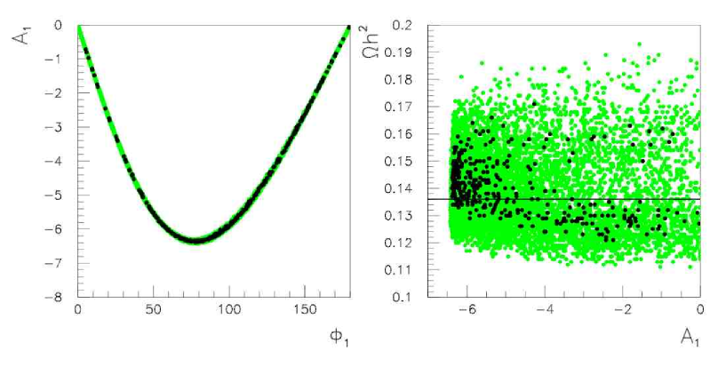
Figure 10: Triple-product asymmetry $A_{1}$ in the $1\sigma$ (black) and $2\sigma$ (green) fitted regions, in (a) as a function of $\phi_{1}$ and in (b) correlation with $\Omega h^{2}$.

In principle, the transverse polarisation of the $\tau$ from the decay $\tilde{\chi}_{2}^{0}\to\tilde{\tau}_{1}\tau$ is sensitive to the phases $\phi_{1},\phi_{\mu},\phi_{\tau}$, and can be large in general [44, 45]. However, since the dependence of the transverse $\tau$ polarization on $\phi_{\tau}$ is weak for $|A_{\tau}|\ll|\mu|\tan\beta$, as in our scenario, we only obtain polarisations not larger than $0.7\%$ for non-vanishing phases, with ${\rm BR}(\tilde{\chi}_{1}^{+}\to\tilde{\nu}_{\tau}\tau^{+})\approx 50\%$.

5.2 Note on chargino production

CP-odd observables in chargino production and decay are in general only sensitive to the phase $\phi_{\mu}$ of the chargino sector. Our scenario actually assumes $\phi_{\mu}=0$. For completeness, we briefly mention how to constrain the phase $\phi_{\mu}$ in principle. Due to the heavy sneutrino mass $m_{\tilde{\nu}_{e}}=1$ TeV, the destructive sneutrino interference term in chargino production $e^{+}e^{-}\to\tilde{\chi}_{1}^{+}\tilde{\chi}_{1}^{-}$ is suppressed, such that the cross section reaches more than $2000$ fb in our scenario for $(P_{e^{-}},P_{e^{+}})=(-0.8,0.6)$ at $\sqrt{s}=500$ GeV. Since all couplings in diagonal chargino pair production are real [46], there is no CP-sensitive contribution from $\phi_{\mu}$ in the production process alone. However, if the chargino decays into polarised particles, viz. the $\tau$, CP-sensitve observables can be defined [47]. Similar to the neutralino decay, one such quantity is the the transverse polarisation of the $\tau$ in the decay $\tilde{\chi}_{1}^{\pm}\to\tau\tilde{\nu}_{\tau}$. In our scenario, the transverse $\tau$ polarisation could be as large as $4\%$ for $\phi_{\mu}=90^{\circ}$.

6 Constraining further the model

In the previous section we have found that the precise determination of a few observables at the ILC still leaves a large uncertainty in the prediction of the relic density of the dark matter candidate. This holds even if CP-odd observables are included. However, at the timescale where the ILC may start its operation, other measurements will be available that could constrain further the model. Below we discuss direct and indirect detection of DM, as well as EDM measurements. Finally, we comment on further measurements of heavy sparticles at the LHC and/or a linear collider with higher energies.

6.1 Direct detection

Upper limits on the cross section for elastic scattering of DM particles on nuclei are improving every year, with the strongest constraints currently coming from Xenon10 [48] and CDMS [49], see also [50]. For a $80$ GeV WIMP, the limit on the spin-independent interaction with protons is $\sigma^{SI}_{p}\;\raisebox{-3.87495pt}{$\textstyle\stackrel{{\scriptstyle\textstyle<}}{{\sim}}$}\;5\times 10^{-8}$ pb [49]. The next generation of detectors should probe $\sigma^{SI}_{p}\approx 10^{-10}$ pb within less than 10 years [51]. Furthermore, the near maximal sensitivities of the detectors are in the mass range of interest here, i.e. around 100 GeV. For spin-dependent interactions, limits are much weaker, about $10^{-2}$ pb [52, 53] with prospects of reaching ultimately $\sigma^{SD}_{p}\approx 10^{-6}$–$10^{-7}$ pb with ton-size detectors, see e.g. [54].

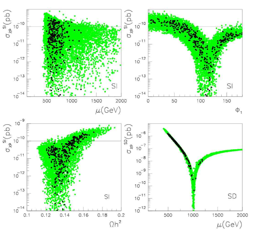
Figure 11: Predictions for $\sigma^{SI}_{p}$, in (a) as a function of $\mu$, in (b) as a function of $\phi_{1}$. In (c) correlation between $\sigma^{SI}_{p}$ and $\Omega h^{2}$. The expected reach of ton-size detectors is indicated. Frame (d) shown predictions for $\sigma^{SD}_{p}$ as a function of $\mu$. As before, the $2\sigma$ ($1\sigma$) fitted region is shown in green (black).

In our scenario, where the squarks of the first two generations are heavy, the spin-independent cross section is completely dominated by the Higgs exchange diagram. We therefore expect $\sigma_{p}^{SI}$ to be sensitive to $\mu$ and $\phi_{1}$ through the $\tilde{\chi}^{0}_{1}\tilde{\chi}^{0}_{1}h$ coupling. Since the LSP couples to the Higgs through its higgsino component, we expect a small cross section in our scenario, where the LSP is dominantly bino. This is indeed the case, as can be seen in Fig. 11. Nevertheless for some of the parameter space the cross section is large enough to be detectable at future ton-size detectors. This occurs mostly for near minimal $\mu$ values, Fig. 11(a). The dependence on the phase $\phi_{1}$, Fig. 11(b), can be related to the suppression of the $\tilde{\chi}^{0}_{1}\tilde{\chi}^{0}_{1}h$ coupling. Furthermore, for near maximal phase there is an interference between the light and heavy Higgs contributions which leads to a strong suppression of the $\tilde{\chi}^{0}_{1}p\rightarrow\tilde{\chi}^{0}_{1}p$ cross section. The models which predict a cross section that could be detected in the near future are precisely those where $\Omega h^{2}$ is the largest, see Fig. 11(c). Since a positive signal is not expected in this particular scenario, we conclude that an improvement on the limit of the neutralino proton elastic scattering would reduce the uncertainty in the prediction of the relic density to $0.116\leq\Omega h^{2}\leq 0.17$, provided the major hadronic uncertainties [55, 56] stemming from the strange content in the nucleon can be brought under control.

The spin-dependent cross section is dominated by $Z$ exchange and hence is also expected to be largest when the higgsino component is largest, that is for small $\mu$. No strong dependence on the phase $\phi_{1}$ appears. Moreover, as shown in Fig. 11(d), the prediction for the spin-dependent cross section is far below the present limit. The $\mu$-dependence is, however, more pronounced than in the spin-independent case. If ambitious projects like [54] can reach $\sim 10^{-7}$ pb, they will indeed probe the small $\mu$ region, where our nominal point lies.

Last but not least note that the cross sections for direct DM detection also depend on the local DM density and velocity distribution. Therefore even a positive DM signal will not directly limit the SUSY parameter space, but rather provide a consistency check.

6.2 Cross sections for indirect detection

For completeness we show in Fig. 12 also the cross section for neutralino annihilation into photons. Here we consider only photons that come from the decays of the neutralino annihilation products. The cross-section is of the order of few times $10^{-26}~{}{\rm cm^{3}/s}$ and vary only by about a factor of two in the $2\sigma$ parameter range. These cross sections are relevant for indirect DM detection experiments such as EGRET [57] or GLAST  [58]. While of course being interesting and useful by itself, indirect detection will not help in pinning down the model parameters. Indeed the rate for $\gamma$-rays detection strongly depends on the model for the neutralino density near the center of the galaxy, predictions can vary by more than an order of magnitude [5] washing out the variations induced by the phase dependence.

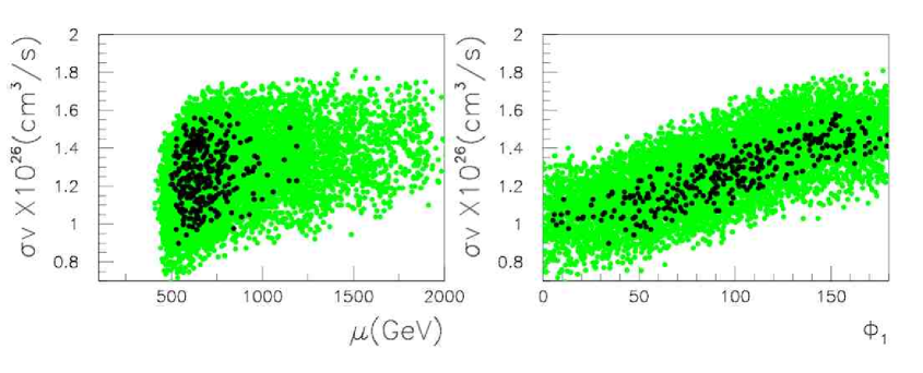
Figure 12: Indirect detection cross sections $\sigma v$ [$cm^{3}/s$] in the $1\sigma$ (black) and $2\sigma$ (green) regions, in (a) as a function of $\mu$, and in (b) as a function of $\phi_{1}$.

6.3 EDMs

We argued in Sect. 2 that EDM constraints are satisfied in our scenario by choosing heavy sfermions of the first and second generations. However, scanning over the parameters of the model we find that for not too large values of $\mu$ and a large phase $\phi_{1}$, the predictions for the Thallium EDM are above the present bound $d_{\rm Tl}<9\times 10^{-25}~{}{\rm e\,cm}$ [59], see Fig. 13(a,b). Taking this bound into account would, however, not much impact the allowed range for $\Omega h^{2}$ as can be seen in Fig. 13(c). Note that here $d_{\rm Tl}$ is computed using $M_{\tilde{e},\tilde{\mu}}\simeq 1$ TeV and that a lack of discovery of sleptons at LHC/ILC will only put a lower bound on the slepton mass. Increasing the slepton masses beyond 1 TeV further weakens the EDM constraint. For this reason we do not include this contraint in our fit but use it only a posteriori. The electron EDM is currently directly extracted from the Thallium measurement, prospects for improving the accuracy on the electron EDM by two orders of magnitude are being explored [60, 61]. Clearly such refined measurements should probe most of the parameter space of the scenario considered.

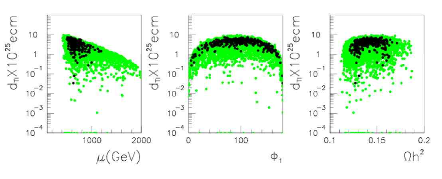
Figure 13: Predictions for $d_{\rm Tl}$ in the $1\sigma$ (black) and $2\sigma$ (green) regions, in (a) as a function of $\mu$ and (b) as a function of $\phi_{1}$. Frame (c) shows the correlation between $d_{\rm Tl}$ and $\Omega h^{2}$.

6.4 Heavy particles at colliders

A large part of the uncertainty in the model reconstruction comes from the lack of knowledge of $\mu$ and $\tan\beta$. Here the obvious ways out would be to i) determine $\tan\beta$ from the Higgs sector and/or ii) determine $\mu$ from a measurement of the higgsino states.

As explained above, to exploit the precision measurement of the light Higgs mass, one would need to know the parameters of the stop sector. Extracting a stop signal is, however, notoriously difficult at the LHC, at least unless $\tilde{t}_{1}$ is very light [62, 63]. This is due to the sheer overwhelming $t\bar{t}$ background. Moreover, even if the stop masses could be measured, this would not be sufficient; one would need in addition a measurement of the stop mixing angle to extract $A_{t}$. This only seems feasible at a multi-TeV $e^{+}e^{-}$ linear collider, such as CLIC [64].

The heavy higgsino-like chargino $\tilde{\chi}^{\pm}_{2}$ and neutralinos $\tilde{\chi}^{0}_{3,4}$ could be detected at the LHC through Drell-Yan production or through squark decays into them. The former suffers from a very small cross section of only few fb, and the latter from tiny branching ratios. It is clear that any such measurement will be very challenging and require very high luminosity.

Alternatively, $\tilde{\chi}^{\pm}_{2}$ or $\tilde{\chi}^{0}_{3,4}$ could be produced in $e^{+}e^{-}$ annihilation with higher energy. The first kinematically accessible process is $\tilde{\chi}^{0}_{1}\tilde{\chi}^{0}_{3,4}$ at about 700 GeV, followed by $\tilde{\chi}^{\pm}_{1}\tilde{\chi}^{\mp}_{2}$ at about 800 GeV. However, the production cross sections are small, below a femtobarn, since one state is almost purely bino or wino and the other higgsino. To be precise, at $\sqrt{s}=800$ GeV one would have $\sigma(e^{+}_{L}e^{-}_{R}\to\tilde{\chi}^{\pm}_{1}\tilde{\chi}^{\mp}_{2})=0.74$ fb and $\sigma(e^{+}_{L}e^{-}_{R}\to\tilde{\chi}^{0}_{2}\tilde{\chi}^{0}_{3})=0.45$ fb, increasing to $1.48$ fb and $0.74$ fb respectively at $\sqrt{s}=1$ TeV. At $\sqrt{s}\geq 1.22$ TeV, one could finally produce the heavier states in pairs, i.e. $\tilde{\chi}^{\pm}_{2}\tilde{\chi}^{\mp}_{2}$, $\tilde{\chi}^{0}_{3}\tilde{\chi}^{0}_{3}$, etc.. The $\tilde{\chi}^{\pm}_{2}\tilde{\chi}^{\mp}_{2}$ cross sections rises fast, giving $\sigma(e^{+}_{R}e^{-}_{L}\to\tilde{\chi}^{+}_{2}\tilde{\chi}^{-}_{2})\simeq 100$ fb at $\sqrt{s}\geq 1.4$ TeV, while $\sigma(e^{+}_{R}e^{-}_{L}\to\tilde{\chi}^{0}_{3}\tilde{\chi}^{0}_{4})\simeq 30$ fb at this energy and the other cross sections much smaller. With such measurements, the complete neutralino/chargino system can in principle be reconstructed [65, 66, 67, 68].

A detailed analysis of LHC measurements or linear collider measurements at TeV energies is beyond the scope of this paper. Notice, however, that for a percent-level collider determination of $\Omega h^{2}$, one would need to know not only $\mu$ and $\tan\beta$ but also the CP phases (in our case $\phi_{1}$) to a comparable, i.e. percent-level, precision.

7 Conclusions

Considering the general MSSM with CP phases, we have investigated a “stau-bulk” scenario, in which only gauginos and staus are light and accessible to ILC measurements, while all other sparticles are heavy. In this scenario, a precise determination of SUSY particle properties is quite challenging at colliders because of the dominance of the channels involving taus and missing energy. Combining threshold scans, endpoint methods, measurements of polarized cross section and tau polarization, the masses of the lightest neutralino, chargino and of both staus can be determined precisely at the ILC. Information on the stau mixing can also be obtained.

From these measurements, some of the underlying Lagrangian parameters can be extracted with good precision: $M_{1}$, $M_{2}$, $M_{\tilde{L}_{3}}$, $M_{\tilde{R}_{3}}$. Moreover, the product $\mu\tan\beta$ can be constrained. However, we are left with a large uncertainty in both $\mu$ and $\tan\beta$, as well as in the phase of $M_{1}$, $\phi_{1}$. This causes a rather large uncertainty in the collider prediction of the neutralino relic density of $0.116<\Omega_{\tilde{\chi}}h^{2}<0.19$ at 95% CL.

Taking into account the possibility of non-zero phases is of particular importance: from pure sparticle spectroscopy, e.g. the measurement of the $\tilde{\chi}^{0}_{1}$–$\tilde{\tau}_{1}$ mass difference which is $\sim 10$ GeV in our scenario, one might conclude that the neutralino relic density is too large, $\Omega_{\tilde{\chi}}h^{2}\;\raisebox{-3.87495pt}{$\textstyle\stackrel{{\scriptstyle\textstyle>}}{{\sim}}$}\;0.14$. Evidence of a CP-violating signal in EDMs and/or in collider measurements would clearly show that phases have to be taken into account. It would, however, not directly add information for infering the relic density of the neutralino dark matter candidate.

We have also discussed implications for (in)direct dark matter searches. While the cross section for indirect detection shows a too weak dependence, information from large scale dark matter detectors could indeed somewhat reduce the allowed parameter range. In any case, direct and indirect detection are important cross checks that the $\tilde{\chi}^{0}_{1}$ is indeed the DM.

Finally, for a percent-level collider determination of $\Omega h^{2}$, which matches the precision of cosmological observations, one would need know also $\mu$, $\tan\beta$, and the CP phases (in our case $\phi_{1}$) to percent-level precision. To this aim, the above-mentioned ILC measurements have to be complemented by precision measurements of the heavy higgsino-like neutralinos and charginos at TeV energies.

References

- [1] WMAP, D. N. Spergel et al., Astrophys. J. Suppl. 170, 377 (2007), [astro-ph/0603449].
- [2] SDSS, M. Tegmark et al., Phys. Rev. D69, 103501 (2004), [astro-ph/0310723].
- [3] WMAP, J. Dunkley et al., arXiv:0803.0586 [astro-ph].
- [4] Planck, astro-ph/0604069.
- [5] G. Bertone, D. Hooper and J. Silk, Phys. Rept. 405, 279 (2005), [hep-ph/0404175].
- [6] D. Hooper and E. A. Baltz, arXiv:0802.0702 [hep-ph].
- [7] G. Polesello and D. R. Tovey, JHEP 05, 071 (2004), [hep-ph/0403047].
- [8] P. Bambade, M. Berggren, F. Richard and Z. Zhang, hep-ph/0406010.
- [9] R. Arnowitt et al., arXiv:0802.2968 [hep-ph].
- [10] H.-U. Martyn, hep-ph/0408226.
- [11] M. M. Nojiri, G. Polesello and D. R. Tovey, JHEP 03, 063 (2006), [hep-ph/0512204].
- [12] E. A. Baltz, M. Battaglia, M. E. Peskin and T. Wizansky, Phys. Rev. D74, 103521 (2006), [hep-ph/0602187].
- [13] C. F. Berger, J. S. Gainer, J. L. Hewett, B. Lillie and T. G. Rizzo, arXiv:0712.2965 [hep-ph].
- [14] T. Falk, K. A. Olive and M. Srednicki, Phys. Lett. B354, 99 (1995), [hep-ph/9502401].
- [15] P. Gondolo and K. Freese, JHEP 07, 052 (2002), [hep-ph/9908390].
- [16] T. Nihei, Phys. Rev. D73, 035005 (2006), [hep-ph/0508285].
- [17] M. E. Gomez, T. Ibrahim, P. Nath and S. Skadhauge, Phys. Rev. D72, 095008 (2005), [hep-ph/0506243].
- [18] G. Belanger, F. Boudjema, S. Kraml, A. Pukhov and A. Semenov, Phys. Rev. D73, 115007 (2006), [hep-ph/0604150].
- [19] U. Chattopadhyay, T. Ibrahim and P. Nath, Phys. Rev. D60, 063505 (1999), [hep-ph/9811362].
- [20] S. Y. Choi, S.-C. Park, J. H. Jang and H. S. Song, Phys. Rev. D64, 015006 (2001), [hep-ph/0012370].
- [21] T. Nihei and M. Sasagawa, Phys. Rev. D70, 055011 (2004), [hep-ph/0404100].
- [22] J. S. Lee et al., Comput. Phys. Commun. 156, 283 (2004), [hep-ph/0307377].
- [23] G. Belanger, F. Boudjema, A. Pukhov and A. Semenov, Comput. Phys. Commun. 176, 367 (2007), [hep-ph/0607059].
- [24] G. Belanger, F. Boudjema, A. Pukhov and A. Semenov, arXiv:0803.2360 [hep-ph].
- [25] J. Hamann, S. Hannestad, M. S. Sloth and Y. Y. Y. Wong, Phys. Rev. D75, 023522 (2007), [astro-ph/0611582].
- [26] ATLAS, CERN-LHCC-99-14.
- [27] M. Bisset, J. Li, N. Kersting, F. Moortgat and S. Moretti, arXiv:0709.1029 [hep-ph].
- [28] F. Moortgat, private communication.
- [29] ECFA/DESY LC Physics Working Group, J. A. Aguilar-Saavedra et al., hep-ph/0106315.
- [30] M. Pohl and H. J. Schreiber, hep-ex/0206009.
- [31] T. Sjostrand et al., Comput. Phys. Commun. 135, 238 (2001), [hep-ph/0010017].
- [32] T. Ohl, Comput. Phys. Commun. 101, 269 (1997), [hep-ph/9607454].
- [33] S. Jadach, Z. Was, R. Decker and J. H. Kuhn, Comput. Phys. Commun. 76, 361 (1993).
- [34] M. M. Nojiri, Phys. Rev. D51, 6281 (1995), [hep-ph/9412374].
- [35] M. M. Nojiri, K. Fujii and T. Tsukamoto, Phys. Rev. D54, 6756 (1996), [hep-ph/9606370].
- [36] E. Boos et al., Eur. Phys. J. C30, 395 (2003), [hep-ph/0303110].
- [37] A. A. Markov, Extension of the limit theorems of probability theory to a sum of variables connected in a chain, reprinted in Appendix B of: R. Howard, Dynamic Probabilistic Systems, volume 1: Markov Chains, John Wiley and Sons, 1971.
- [38] N. Metropolis, A. W. Rosenbluth, M. N. Rosenbluth, A. H. Teller and T. E., Equations of state calculations by fast computing machines, Journal of Chemical Physics, 21 (1953) 1087-1092.
- [39] W. K. Hastings, Monte carlo sampling methods using markov chains and their applications, Biometrika, 57(1):97–109, 1970.
- [40] see also C.G. Lester, M.A. Parker, M.J. White, JHEP 0601 (2006) 080.
- [41] Y. Kizukuri and N. Oshimo, Phys. Lett. B249, 449 (1990).
- [42] A. Bartl, H. Fraas, O. Kittel and W. Majerotto, Phys. Rev. D69, 035007 (2004), [hep-ph/0308141].
- [43] J. A. Aguilar-Saavedra, Nucl. Phys. B697, 207 (2004), [hep-ph/0404104].
- [44] A. Bartl, T. Kernreiter and O. Kittel, Phys. Lett. B578, 341 (2004), [hep-ph/0309340].
- [45] S. Y. Choi, M. Drees, B. Gaissmaier and J. Song, Phys. Rev. D69, 035008 (2004), [hep-ph/0310284].
- [46] S. Y. Choi, A. Djouadi, H. S. Song and P. M. Zerwas, Eur. Phys. J. C8, 669 (1999), [hep-ph/9812236].
- [47] A. Marold et al., in preparation.
- [48] XENON, J. Angle et al., Phys. Rev. Lett. 100, 021303 (2008), [arXiv:0706.0039 [astro-ph]].
- [49] CDMS, Z. Ahmed et al., arXiv:0802.3530 [astro-ph].
- [50] D. Butler, J. Filippini and R. Gaitskel, http://dmtools.brown.edu/.
- [51] H. Kraus et al., Nucl. Phys. Proc. Suppl. 173, 168 (2007).
- [52] ZEPLIN-II, G. J. Alner et al., Phys. Lett. B653, 161 (2007), [arXiv:0708.1883 [astro-ph]].
- [53] CDMS, D. S. Akerib et al., Phys. Rev. D73, 011102 (2006), [astro-ph/0509269].
- [54] COUPP, J. Collar et al., FERMILAB-PROPOSAL-0961.
- [55] A. Bottino, F. Donato, N. Fornengo and S. Scopel, Astropart. Phys. 18, 205 (2002), [hep-ph/0111229].
- [56] J. Ellis, K. A. Olive and C. Savage, arXiv:0801.3656 [hep-ph].
- [57] P. Sreekumar, F. W. Stecker and S. C. Kappadath, AIP Conf. Proc. 510, 459 (2004), [astro-ph/9709258].
- [58] GLAST-LAT, A. Morselli, A. Lionetto and E. Nuss, AIP Conf. Proc. 921, 181 (2007).
- [59] B. C. Regan, E. D. Commins, C. J. Schmidt and D. DeMille, Phys. Rev. Lett. 88, 071805 (2002).
- [60] D. Kawall, F. Bay, S. Bickman, Y. Jiang and D. DeMille, Phys. Rev. Lett. 92, 133007 (2004), [hep-ex/0309079].
- [61] S. K. Lamoreaux, physics/0701198.
- [62] S. Kraml and A. R. Raklev, Phys. Rev. D73, 075002 (2006), [hep-ph/0512284].
- [63] B. C. Allanach et al., hep-ph/0602198.
- [64] CLIC Physics Working Group, E. Accomando et al., hep-ph/0412251.
- [65] J. L. Kneur and G. Moultaka, Phys. Rev. D61, 095003 (2000), [hep-ph/9907360].
- [66] S. Y. Choi et al., Eur. Phys. J. C14, 535 (2000), [hep-ph/0002033].
- [67] S. Y. Choi, J. Kalinowski, G. A. Moortgat-Pick and P. M. Zerwas, Eur. Phys. J. C22, 563 (2001), [hep-ph/0108117].
- [68] S. Y. Choi, J. Kalinowski, G. A. Moortgat-Pick and P. M. Zerwas, hep-ph/0202039.