Random Vortex-Street Model for a Self-Similar Plane Turbulent Jet

Abstract

We ask what determines the (small) angle of turbulent jets. To answer this question we first construct a deterministic vortex-street model representing the large scale structure in a self-similar plane turbulent jet. Without adjustable parameters the model reproduces the mean velocity profiles and the transverse positions of the large scale structures, including their mean sweeping velocities, in a quantitative agreement with experiments. Nevertheless the exact self similar arrangement of the vortices (or any other deterministic model) necessarily leads to a collapse of the jet angle. The observed (small) angle results from a competition between vortex sweeping tending to strongly collapse the jet and randomness in the vortex structure, with the latter resulting in a weak spreading of the jet.

Introduction: We address the apparent universality of the self-similar structure of plain turbulent free jet. It had been amply documented65brad ; 76GW ; 82OG ; Pope ; 00GT ; 86TB ; 81GYO that such jets contain dynamically dominant large-scale self-organized motions consisting of two lines of large-scale vortices centered at staggered position on the two sides of the jet: $y(x)=\pm a\,b(x)\,,\quad b(x)=\alpha\,x\,,\ a\approx 0.85$, where $x$ is a stream-wise coordinate, $b(x)$ is the jet half-width footnote and $\alpha$ is the jet angle. This structure carries about 75% of the total kinetic energy 00GT . Importantly, the remaining turbulent energy randomizes in part the positions and amplitudes of the coherent vortices.

In this Letter we first construct a deterministic vortex-street model that excellently reproduces the experimentally observed longitudinal mean velocity profile without any adjustable parameter. The model predicts the transverse positions of the large scale structures, including their mean sweeping velocities, in a quantitative agreement with experiments. Nevertheless both the existence of a regular array of vortices and the turbulent randomization are crucial for understanding the (relatively small) observed angle $\alpha_{\text{exp}}\approx 0.1$ of the jet spreading. Therefore, secondly we develop a random-vortex street model, that leads to an estimate of the jet angle $\alpha_{\text{mod}}\approx 0.13$ (reasonably close to the observed angle) as a result of a competition between the regular and the stochastic components.

The deterministic model: To model the coherent structure of a plane jet we employ vortices with a finite core size 82OG . Here we choose a simple algebraic model for the vorticity $\omega(r)$ and angular velocity $v_{\varphi}(r)$ that allows an analytic treatment:

$$\omega(r)=\frac{\Gamma c^{4}}{\pi(r^{4}+c^{4})^{3/2}}\ \Rightarrow\ v_{\varphi}(r)=\frac{\Gamma\,r}{2\pi\sqrt{r^{4}+c^{4}}}\ ,$$ (1)

where $r$ is the distance from the vortex center. To characterize the self-similar structure of the jet we enumerate the vortices by their sequential number $-\infty<n<\infty$ and introduce a scaling parameter $\lambda>1$ such that the $x$-position of vortex centers are $x_{n}=x_{0}\lambda^{n}$, where $x_{0}$ is the stream-wise position of a reference vortex. The $y$-position of the vortices is chosen at the points of inflection of the mean velocity profile where the production of vorticity has its maximum: $y_{n}=(-1)^{n}a\,\alpha\,x_{n}$, where both $a$ and $\alpha$ need to be determined below.

Note that we construct the jet exactly self-similar; in experiments this is achieved only asymptotically away from the orifice, about 30 times the width of the orifice. To flush out the scaling properties of the mean stream-wise velocity $V_{x}(x,y)$ and the velocity circulation $\Gamma_{n}$ notice that for the free jet the stream-wise momentum flux $M$ is $x$-independent:

$$M\equiv\int_{-\infty}^{\infty}V_{x}(x,y)^{2}dy\approx~{}V_{x}(x,0)^{2}b(x)\ .$$ (2)

Since $b(x)$ scales as $x$, for constant $M$ the centerline velocity $V_{x}(x,0)$ should necessarily scale like $1/\sqrt{x}$. Similarly, one estimates $\Gamma_{n}\sim V_{x}(x_{n},0)b(x_{n})\propto\sqrt{x_{n}}\propto\sqrt{\lambda^{n}}$. Therefore $\Gamma_{n}=\gamma(-\sqrt{\lambda})^{n}$, with some dimensional constant $\gamma$.

Note that this model, if used as initial condition for the Euler equation, will lose its self-similarity immediately. Dynamically suitable model that reflects the self similarity of the observed jet will call for a very very much more detailed and parameterized description. The analytic simplicity of the present model results from the fact that the self-similarity should be interpreted statistically rather than dynamically; in the real jet situation we must allow for the coalescence or sometime creation or death of vortices.

At an arbitrary position $x,\ y$ and time $t$ the stream-wise velocity field, produced by all the vortices, is:

$$U_{x}(x,y) = \frac{\gamma}{2\pi}\sum_{n}{-(-\sqrt{\lambda})^{n}Y_{n}}\big{/}{R_{n}^{2}}\,,$$ (3a)

$$R_{n}^{2} \equiv \sqrt{\left({X_{n}}^{2}+{Y_{n}}^{2}\right)^{2}+c^{4}}\,,$$ (3b)

$$X_{n} \equiv x-x_{n}\,,\quad Y_{n}\equiv y-y_{n}\,,$$ (3c)

where the core radius of the $n$-th vortex $c_{n}=c_{0}\lambda^{n}$. Similarly one gets an equation for the transverse velocity $U_{y}(x,y)$ by replacing $-Y_{n}\to X_{n}$ in the numerator of Eq. (3).

We define the mean (in time) velocity profiles, $V_{x}(x,y)\equiv\langle U_{x}(x,y)\rangle$ and $V_{y}(x,y)\equiv\langle U_{y}(x,y)\rangle$ and the normalized coordinates $\xi\equiv x/b(x),\zeta\equiv y/b(x)$. As the next step we define a normalized self-similar mean velocity, which is $x$-independent in the self-similar regime:

$${\bm{V}}^{\ddagger}(\zeta)\equiv{\bm{V}}(x,y/b(x))/V_{x}(x,0)\,.$$ (4)

Since the actual experimental value of the spreading angle $\alpha_{\text{exp}}$ is small, and since we will find below that the profile of the longitudinal mean velocity is very weakly dependent on $\alpha$, it is very worthwhile to proceed and analyze precisely the limit $\alpha\to 0$, where the vortices are arranged on two parallel lines $y=\pm a$, separated in the streamvise direction by $d$. There we can simplify dramatically the calculation of the mean stream-wise velocity from Eq. (3), in the form of a single integral. For $\alpha\to 0$ we write $\lambda^{n}\to 1+(\lambda-1)n$ and substitute in Eq. (3) $x_{n}=x_{0}+n\,d\,b$, $d=(\lambda-1)x_{0}$, $y_{n}=(-1)^{n}ab$, $c_{n}=c\,b$, where $b$ is the $x$-independent jet half-width:

$${\mathcal{U}}_{x}(x,y)=\frac{\gamma}{2\pi b}\sum_{n=-\infty}^{\infty}\frac{{\mathcal{Y}}_{n}}{{\mathcal{R}}_{n}}\,, {\mathcal{Y}}_{n}\equiv a-(-1)^{n}\zeta\,,$$ (5a)

$${\mathcal{U}}_{y}(x,y)=\frac{\gamma}{2\pi b}\sum_{n=-\infty}^{\infty}\frac{{\mathcal{X}}_{n}}{{\mathcal{R}}_{n}}, \!\!\!{\mathcal{X}}_{n}\equiv(-1)^{n}(\xi-nd)\,,~{}~{}~{}~{}$$ (5b)

$${\mathcal{R}}^{2}_{n} \equiv \sqrt{\left({\mathcal{X}}_{n}^{2}+{\mathcal{Y}}_{n}^{2}\right)^{2}+c^{4}}\ .$$ (5c)

The average with respect to time was replaced by averaging in the $\xi$ direction over one period of oscillations (between two consecutive vortices at $-d$ and $d$). In each term in the sum (separately for odd and even $n$) we can change the integration variables $\xi^{\prime}=\xi+2\,d\,n$ and eventually collapse the whole sum into two integrals, finding for ${\mathcal{V}}_{x}(b\,\zeta)\equiv\langle{\mathcal{U}}_{x}(x,y)\rangle$:

$${\mathcal{V}}_{x}(b\,\zeta) = \frac{\gamma}{4\pi b\,d}[I^{+}(\zeta)+I^{-}(\zeta)]\,,$$ (6a)

$$I^{\pm}(\zeta) = \int_{-\infty}^{\infty}A_{\pm}d\xi\,,$$ (6b)

$$A_{\pm} \equiv {(\zeta\pm a)}\big{/}{\sqrt{[(\zeta\pm a)^{2}+\xi^{2}]^{2}+c^{4}}}\ .$$ (6c)

Notice that ${\mathcal{V}}_{y}(\zeta)$ vanishes in the limit $\alpha\to 0$ due to symmetry. While these results were developed for the limit $\alpha\to 0$, we will demonstrate that they pertain excellently well also for small $\alpha$. The normalized profile according to Eqs. (4) and (6a):

$${\mathcal{V}}_{x}^{\ddagger}(\zeta)\equiv{[I^{+}(\zeta)+I^{-}(\zeta)]}/{[I^{+}(0)+I^{-}(0)]}\ .$$ (7)

This profile depends only on $a$ and $c$. With the definition of the width of the jet, $b(x)$, we now demand ${\mathcal{V}}_{x}^{\ddagger}(1)=\frac{1}{2}$, giving us one relation between $a$ and $c$. The second relation between these parameters is determined by the position of the inflection point: $d^{2}{\mathcal{V}}_{x}^{\ddagger}(\zeta)/d\zeta^{2}=0$ at $\zeta=a$. Solving the two conditions together we find $a=0.747$ and $c=1.1$. The resulting profile (7) with these values of the parameters is shown in Fig. 1.

Figure 1: Color online. Profiles of the normalized stream-wise mean velocity: Black squares – experimental points 00GT , black dashed line – profile (9) obtained from the Prandtl closure with constant turbulent viscosity approximation, red dash-dotted line line – Eq. (7) ($\alpha\to 0$ limit) with $a=0.747$, $c\approx 1.1$. Black solid line – profile (8) with $\alpha=0.1$ and the same values of $a$ and $c$.

This profile ${\mathcal{V}}_{x}^{\ddagger}(\zeta)$ obtained for $\alpha=0$ should be compared to the profile $V_{x}^{\ddagger}(\zeta)$ computed for finite $\alpha$ note1 :

$$V_{x}^{\ddagger}(\zeta) = {[J^{+}(\zeta)+J^{-}(\zeta)]}\big{/}{[J^{+}(0)+J^{-}(0)]}\,,$$ (8)

$$J^{\pm}(\zeta) \equiv \int\limits_{0}^{\infty}\frac{d\chi}{\alpha\sqrt{\chi}}\,\frac{a\chi\pm\zeta}{\sqrt{[(a\chi\pm\zeta)^{2}+(\chi-1)^{2}/\alpha^{2}]^{2}+c^{4}\chi^{4}}}\ .$$

In Fig. 1 we compare these two profiles and find that as expected they are practically indistinguishable for the experimental value $\alpha_{\rm exp}=0.1$. Moreover, the profile Eq. (8) is almost insensitive to $\alpha$ for small $\alpha\lesssim 0.15$. In the same figure we compare the model profile to the experimental data 00GT , and find excellent agreement. In contrast, the profile

$$V_{{\rm utv},x}^{\ddagger}(\zeta)=\cosh^{-2}\Big{[}\zeta\,\ln(1+\sqrt{2})\Big{]}\ ,$$ (9)

computed using the “uniform turbulent viscosity” assumption note2 , deviates strongly from the data for $\zeta>1$.

Moreover, the present model fits the data in more than one way. One can actually measure the transverse positions $y_{n}$ of the large scale vortices in units of the $b(x_{n})$. In the self-similar regime of the jet the ratio $y_{n}/b(x_{n})$ is $n$-independent and best estimates 00GT give approximately 0.85 in a reasonable agreement with our value of $a\approx 0.75$. Finally, the measured value of the stream-wise velocity of the coherent structures in units of the centerline velocity is about $0.60-0.65$ 86TB ; 81GYO . Our model predicts ${\mathcal{V}}_{x}^{\ddagger}(a)\approx 0.57$. We remind the reader that all this agreement is achieved without using any experimental data.

Figure 2: Vortex structure (a fragment from experimental proper orthogonal decomposition, Ref. 00GT ).

Having modeled so successfully the stream-wise velocity, we can now evaluate the transverse velocity by using the incompressibility constraint and Eq. (4). We derive

$$V_{y}^{\ddagger}(\zeta)=\frac{\alpha}{2}\int_{0}^{\zeta}d\widetilde{\zeta}\,\Big{[}V_{x}^{\ddagger}(\widetilde{\zeta})+2\,\widetilde{\zeta}\,{d\,V_{x}^{\ddagger}(\widetilde{\zeta})}\big{/}{d\widetilde{\zeta}}\Big{]}\ .$$ (10)

For small $\alpha$ one can neglect the $\alpha$ dependence of the integrand in the right hand side of Eq. (10), replacing $V_{x}^{\ddagger}$ by its $\alpha\to 0$ limit ${\mathcal{V}}_{x}^{\ddagger}$. Now we can compute the ratio $\alpha^{\prime}\equiv V_{y}(x,y)/V_{x}(x,y)$ at $y=a\,b(x)$, finding that the sweeping angle of the vortices $\alpha^{\prime}\approx 0.3\,\alpha$ is considerably smaller than the angle $a\,\alpha\approx 0.75\,\alpha$ that is required to preserve the angle self-similarly. This result means that the mean velocity of the vortices is not maintaining the self-similar structure at any (small) value of $\alpha$, tending to collapse the structure to two parallel lines. We expect this result to be generic for any deterministic model.

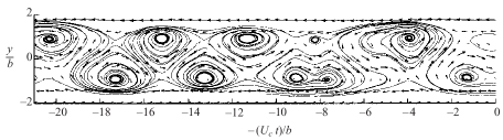
Random Vortex-Street Model. Now we have to account for the fact that the real jet does not display ideal vortex-street structure, see, e.g. Fig. 2. The parameters of individual vortices fluctuate, and we also see the coalescence of vortices as mentioned above. Moreover, pairs of vortices have finite life-time, as we see in Fig. 2, that two vortices are about to disappear at $U_{c}t\approx-8\,b$. We reiterate that the finiteness of the vortex life-time is required by the self-similarity, i.e. the sweeping velocity is oriented along the line that connects the vortex centers. Indeed, the sweeping velocity scales like $1/\sqrt{x}$, the vortex density scales like $1/x$, therefore the flux of the vortex number scales like $1/x^{3/2}$ i.e. decreases with $x$. This means that vortices disappear during their sweeping downstream, i.e. they have finite life time, due to their coalescence, or decay, or whatever. It means, as said above, that self-similar jet structure must be understood in the statistical sense and randomness of the vortex parameters is a necessarily element of the jet structure. The relative success of the deterministic vortex-street model was possible because fluctuations of the vortex parameters have little consequences on the mean values; they can be neglected in zeroth-order approximation in describing the mean velocity profiles. This is not the case for the spreading angle $\alpha$, which tends to collapse in the deterministic limit.

To find the spreading angle $\alpha$ we should consider the normalized velocity fluctuations in the transverse direction $y$,

$$K(x,y) \equiv \left\langle\overline{U_{y}-V_{y})^{2}}\right\rangle=\left\langle\overline{U_{y}^{2}}\right\rangle-V_{y}^{2}\,,$$ (11a)

$$K^{\ddagger}(\zeta) \equiv K(x,y)\big{/}V_{x}(x,0)^{2}\ .$$ (11b)

One simple way to introduce randomness in the model is to account for the fluctuations of the core size of the vortices, $c_{n}=c\,(1+\delta_{n})$ with uncorrelated statistical fluctuations: $\overline{\delta_{n}}=0\,,\quad\overline{\delta_{n}\delta_{n^{\prime}}}\equiv\delta^{2}\Delta_{n,n^{\prime}}$. In the limit $\alpha\to 0$ we replace the parameter $c$ in ${\mathcal{R}}^{2}_{n}$ by $c_{n}$ and (for small fluctuations, $\delta^{2}\ll 1$ ) expand Eqs. (5) with respect of $\delta_{n}$. Averaging the result with respect to the fluctuations and over longitudinal position in the jet we get:

$$\left\langle\overline{U_{y}^{2}}\right\rangle = \left(\frac{\gamma}{2\,\pi\,b}\right)^{2}\frac{1}{2d}\int\limits_{-d}^{d}d\xi\sum_{n,n^{\prime}=-\infty}^{\infty}{\mathcal{X}}_{n}{\mathcal{X}}_{n^{\prime}}E_{n,n^{\prime}}\,,$$ (12a)

$$E_{n,n^{\prime}} \equiv E_{n,n^{\prime}}^{\text{reg}}+E_{n,n^{\prime}}^{\text{ran}}\,,\quad E_{n,n^{\prime}}^{\text{reg}}\equiv\frac{1}{{\mathcal{R}}^{2}_{n}{\mathcal{R}}^{2}_{n^{\prime}}}\,,$$ (12b)

$$E_{n,n^{\prime}}^{\text{ran}} \equiv 2\,\delta^{2}\Big{\{}\frac{2c^{6}\Delta_{n,n^{\prime}}}{{\mathcal{R}}_{n}^{12}}+\frac{3\,c^{2}\big{[}c^{4}-({\mathcal{X}}_{n}^{2}+{\mathcal{Y}}_{n}^{2})^{2}\big{]}}{{\mathcal{R}}_{n}^{10}{\mathcal{R}}^{2}_{n^{\prime}}}\Big{\}}\ .$$

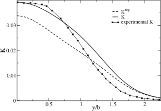
In accordance with these results we present $K$ as a sum of the regular part $K^{\text{reg}}$, that originates from $x$-periodic velocity fluctuations, and the random part $K^{\text{ran}}$, that originates in our model from statistical fluctuations of the core radius: $K=K^{\text{reg}}+K^{\text{ran}}$. Here $K^{\text{reg}}\equiv\left\langle\overline{U_{y}^{2}}\right\rangle^{\text{reg}}-V_{y}^{2}$ and $K^{\text{ran}}\equiv\left\langle\overline{U_{y}^{2}}\right\rangle^{\text{ran}}$, where $\left\langle\overline{U_{y}^{2}}\right\rangle^{\text{reg}}$ and $\left\langle\overline{U_{y}^{2}}\right\rangle^{\text{ran}}$ are related in Eqs. (12) with $E_{n,n^{\prime}}^{\text{reg}}$ and $E_{n,n^{\prime}}^{\text{ran}}$. Experimental information about $K$ is provided in Fig. 3. We see from the data that on the axis of the jet $K^{\ddagger}\approx 0.04$ and at the centers of the vortices $K^{\ddagger}(\zeta=a)\approx 0.03$. We use this data to fix the parameters of the model with the results $d=1.45$ and $\delta^{2}=0.03$. With these parameters the regular contribution $K^{\text{reg}}(a)\approx 0.024$ while the random contribution is considerably smaller, $K^{\text{ran}}(a)\approx 0.006$.

Figure 3: Experimental profile 00GT of the mean square of the cross-stream component of the fluctuating velocity (dots connected by line). In a continuous line we present the profile predicted by the random model. The dashed line is the profile of the regular contribution. The difference at $a$ is the source of spreading of the jet, cf. Eq. (13).

In this way we have separated the regular contribution to $K$ that does not effect the spreading angle, from the random one, $K^{\text{ran}}$, that leads to the jet spreading by turbulent diffusion with a characteristic velocity $\sqrt{K^{\text{ran}}}$. We thus estimate

$$\alpha_{\text{mod}}\simeq\frac{\sqrt{K^{\text{ran}}(a)}}{V_{x}(a)}=\frac{\sqrt{{K_{y}^{\ddagger}}^{\text{ran}}(a)}}{V^{\ddagger}_{x}(a)}\approx 0.13\ .$$ (13)

This estimate of the tangent of the angle of the jet is slightly higher than the experimental value (about 0.1). We note however that we made no effort to model quantitatively the random structure of the vortices. For example, looking at Fig. 2 we note that the vortices are elliptic rather than round, this will definitely contribute to lowering the random part of $K^{\ddagger}$. One could input this knowledge, with a price of additional fit parameters. We submit to the reader that this is not the goal of the present calculation, we are not interested here in a quantitative model of a jet spreading. We wanted to understand what is the physical reason for this phenomenon and why the jet angle is small. We believe that the model worked out above is sufficient; our answer is that any deterministic model will necessarily close the jet angle, allowing only a self similar parallel jet. The reason for the opening angle is randomness, which is the flip side of turbulence which cannot be avoided even when 75% of the energy is in the coherent structure. The randomness contributes partially to the value $K^{\ddagger}$, which is rather small per se. Therefore ${K^{\ddagger}}^{\text{ran}}$ (without which the opening angle will tend to zero) is even smaller and thus resulting spreading angle (13) is indeed small.

Summary. In this Letter we offered a simple model of a plane jet with the aim of understanding the fundamental existence of a statistically self similar structure with a small opening angle. The deterministic part of the model excellently reproduces the experimental profiles of the mean velocity without using any adjustable parameter. For an opening angle we must introduce randomness. In the context of the present simple model we ascribed the randomness to the core size, and demonstrated that this is sufficient to provide an opening angle of the correct order of magnitude. Needless to say we do not pretend that this model describes correctly the full randomness which is due to turbulence, but only underlines the crucial role of the random components in opening up the jet. One can provide a more precise model with better agreement with the measured angle and the profiles of second order quantities, but this calls for additional adjustable parameters. Such a detailed model is not the aim of this Letter which concentrated on understanding the basic physics of the phenomenon.

Acknowledgement. IP thanks Roddam Narasimha for presenting this riddle, and acknowledges partial support by the US-Israel BSF. Additional support was given by the Transnational Access Programme at RISC-Linz, funded by European Commission Framework 6 Programme for Integrated Infrastructures Initiatives under the project SCIEnce (Contract No. 026133).

References

- (1) L.J.S, Bradbury, Journal of Fluid Mechanics, 23, 31 (1965).;
- (2) E. Gutmark,I. Wygnanski,Journal of Fluid Mechanics, 73, 45, (1976).
- (3) J. W. Oler, and V.W. Goldschmidt, V. W. J. Fluid Mech. 123, 523 (1982).
- (4) F.O. Thomas,E.G. Brehob., Phys. Fluids, 29, 1788 (1986);
- (5) V.W. Goldshmidt.M.F. Young, E.S. Ott, J. Fluid Mech. 108,327 (1981)
- (6) S. B. Pope, Turbulent flows (Cambridge Univ. Press, 2000) and references therein.
- (7) S. V. Gordeyev and F. O. Thomas, J. Fluid Mech. 414, 145 (2000) and 460, 349 (2002)
- (8) By definition the half jet width is the cross-stream position at which the stream-wise mean velocity is half of its center-line value.
- (9) Equation for can be obtained from Eq. (3) similarly to Eq. (7). For the profile (8) and a given the values of and were found by the procedure described in the text. It turns out that for small () the values of and practically coincide with the corresponding values for . In the limit the main contribution to the integrals is due to the region . Introducing in Eq. (8) a dummy variable one sees that and profile .
- (10) Using the Prandtl closure in the balance equation for the mechanical moment and assuming that the turbulent viscosity is constant in the jet, one predicts a universal, -independent profile, see e.g. Eq. (5.187) in Pope