A circle of interacting servers; spontaneous collective behavior in case of large fluctuations

Abstract

We consider large fluctuations, namely overload of servers, in a network with dynamic routing of messages. The servers form a circle. The number of input flows is equal to the number of servers, the messages of any flow are distributed between two neighboring servers, upon its arrival a message is directed to the least loaded of these servers. Under the condition that at least two servers are overloaded the number of overloaded servers in such network depends on the rate of input flows. In particular there exists critical level of input rate that in case of higher rate most probable that all servers are overloaded.

Keywords: Large Deviation Principle, Queuing Networks, Dynamic Routing.

1 Introduction

This work presents an effect in a network with interacting servers that can be called a spontaneous collective behavior in case of large fluctuations.

We consider networks with dynamic routing of messages. In such networks the server to which a message is directed depends on the network’s state at the message arrival moment. One of the problems arising here is the analysis of probability of large fluctuations, for example probability of large delays.

There are many works where large fluctuations in networks with dynamic routing have been investigated. In [1] - [9] the networks with two servers and three independent input flows have been considered where only one flow is divided between two servers depending either on the workload of servers or on the queue lengths. In [10] a network with a group of servers and several flows has been considered where each flow is assigned to some subgroup of servers; upon its arrival a message selects a server with the shortest queue(i.e. a queue with least number of messages). In this work the large deviation principal for the flows upon the servers is proved. We would like to stress that the service time of messages in [10] is exponentially distributed. That allows to use Markov property for the flows to servers (after splitting of the input flows.)

The more full list of references can be found in the mentioned works.

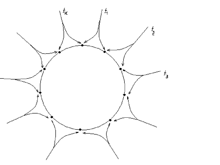
Figure 1:

Here we consider circle networks that are formed by $k$ servers and $k$ identical independent input Poisson flows. Messages of any flow are assigned to two nearby servers (see Figure 1) A message direction depends on the workloads on these two servers, namely upon its arrival a message is directed to the server with the smallest workload. The constant speed of work of each server is equal to 1, the discipline is ”first in - first out” (FIFO). If a message finds the server busy it is put into a infinite buffer to wait for service. We consider the networks that work stationary. That means that with probability 1 the queues do not increase infinitely. But there may appear large fluctuations, for example during a short period one of flows may bring very large amount of work. We say that during this period the flow is overheated. Suppose for example that the flow $f_{1}$ is overheated. Then the buffers of servers $s_{1}$ and $s_{k}$ that are assigned to this flow will contain a large amount of work. What is the behavior of other flows ?

In this paper we show that in case where $f_{1}$ is overheated there exist at least two scenarios of network performance. What scenario is more probable and is realized depends on the rate of input flows. Namely, we show that there exists such value of input flow rate that in case when the arrival rates are above it the overheating of flow $f_{1}$ coincides with overheating of all flows. Such behavior may be regarded as the spontaneous appearance of collective behaviour. On the other hand in case of low rate the overheating of $f_{1}$ does not bring the overheating of other flows. There may exist also intermediate stages where the overheating of one flow coincides with the overheating of a number of neighboring flows. The existence of such intermediate stages depends on message length distribution of input flows. For some length distributions, for example for exponential one, the intermediate stages do not exist.

The proof of this result is based on large deviation principle of [11] (see also [12]). We do not present the details of this reduction. The details of application of large deviation principle for several other problems one can fined in [11, 6, 7]. Instead of the proof we present some ideas needed for the proof and some fragments of rigorous arguments. Therefore the following text is not a proof in the conventional sense.

In the next section we introduce several concepts and definitions and describe the main ideas of our approach. In section 3 several examples are presented.

2 Cyclic networks. Main result

The cyclic network of size $k,\ k\geq 3,$ is formed by $k$ servers and $k$ input flows. Let $F=\{f_{1},...,f_{k}\}$ be the set of flows and $S=\{s_{1},...,s_{k}\}$ the set of servers. All servers work with speed 1, the discipline is FIFO. Each server has an infinite buffer. The messages of flow $f_{i}\in F$ are served by two servers $s_{i}\in S$ and $s_{i-1}\in S$ (here always $i\mp 1\mod k$). Each message of $f_{i}$ is directed to that of servers $s_{i},\ s_{i-1}$ which becomes idle first.

Let the random sequence $(\xi_{n}^{i},\tau_{n}^{i})$, $n=...,-1,0,1,...$, describes the input flow $f_{i}\in F$. The random variables $\tau_{n}^{i}$ are the intervals between the arrivals of messages of flow $f_{i}$. The random variables $\xi_{n}^{i}$ are the lengths of messages. We consider homogeneous Poisson flows therefore all $(\xi_{n}^{i},\tau_{n}^{i})$ are independent and equally distributed, $\tau_{n}^{i}$ are exponentially distributed with rate $\lambda$, i.e. $\Pr(\tau_{n}^{i}>t)=e^{-\lambda t}$. The distributions of input flow do not depend on $i$.

Introduce a random pair $(\xi,\tau)$ that is distributed as any pair $(\xi_{n}^{i},\tau_{n}^{i})$. Each sequence $(\xi_{n}^{i},\tau_{n}^{i})$ is numbered so that $\tau_{0}^{i}<0$ and $\tau_{1}^{i}\geq 0$.

We propose that $\xi$ has exponential moments, i.e. there exist such $\theta_{+}$,   $0<\theta_{+}\leq\infty$ that

$$\varphi(\theta)={{\bf{E}}}e^{\theta\xi}<\infty\ \ \mbox{ for}\ \ \theta<\theta_{+},$$

$$\lim_{\theta\uparrow\theta_{+}}\varphi(\theta)=\infty.$$ (1)

The condition that guarantees the stationarity and even ergodicity is

$$\lambda\varphi^{\prime}(0)<1.$$ (2)

This condition is intuitively obvious but its sufficiency for the existence of stationary stage needs a proof. In particular one may construct a Liapunov function that shows that with large probability the workloads of all stations are located in a compact region. We omit this construction.

To formulate the problem that is investigated we introduce a notion of virtual message. That is a message that arrives with flow $f_{i}$ at a nonrandom time moment, for example at 0 and has zero length. It joins a queue at $s_{i}$ or $s_{i-1}$, depending on where the workload is less, and waits there its service. Let $\omega_{i}$ be the $i$th virtual message’s waiting time. We are interested in the probability of large waiting for virtual massage that arrived with $f_{1}$, i.e. $\Pr(\omega_{1}\geq d)$, where $d$ is large. In some cases, for special choice of $\xi$ distribution the needed probability can be calculated. But in general case it is impossible to present the explicit expression. Therefore one looks for the asymptotics of probability

$$\Pr(\omega_{1}>nd),$$ (3)

where $n\to\infty$. More detailed , one looks for

$$J=\lim_{n\to\infty}\frac{-1}{n}\ln\Pr(\omega_{1}\geq nd).$$ (4)

This problem belongs to the theory of large deviation. We use this theory even where it is possible to get an explicit solution.

2.1 Collective fluctuations

Next theorem states the existence of input flow values $\lambda_{k}\leq\lambda^{k}$ such that separate different types of system performance. Let

$$\hat{\lambda}=\frac{1}{\varphi^{\prime}(0)}.$$

As we mentioned before the system performance is stationary if $\lambda<\hat{\lambda}$.

We say that the flow $f_{i}$ is overheated at $t=0$ if $\Gamma_{i}(n)=(\omega_{i}\geq nd)$. It means that a virtual message that arrived with $f_{i}$ is waiting for being served at least $nd$. Let $\overline{\Gamma}_{i}(n)$ be the complement to event $\Gamma_{i}(n)$.

Theorem 1

. For any system size $k,\;k\geq 3$

and for any $d$ there exist $\lambda_{k},\,\lambda^{k}$ (not depending on $d$), such that $0<\lambda_{k}\leq\lambda^{k}<\widehat{\lambda}$, and

1. if $\lambda<\lambda_{k}$ then

   1. $\Pr\left(\Gamma_{1}(n)\bigcap_{i=2}^{k}\overline{\Gamma}_{i}(n)\,\big{|}\Gamma_{1}(n)\right)\to 1$, as $n\to\infty$.
      

   2. $J=\lim_{n\to\infty}\frac{-1}{n}\ln\Pr\left(\Gamma_{1}(n)\bigcap_{i=2}^{k}\overline{\Gamma}_{i}(n)\right)=2\theta(\lambda,1)d$
      where $\theta(\lambda,1)$ is a positive root to equation

      $$2\theta=\lambda[\varphi(\theta)-1],$$ (5)

2. if $\lambda>\lambda^{k}$ then

   1. $\Pr\left(\bigcap_{i=1}^{k}\Gamma_{i}(n)\,\big{|}\Gamma_{1}(n)\right)\to 1$ as $n\to\infty$,

   2. $J=\lim_{n\to\infty}\frac{-1}{n}\ln\Pr\left(\bigcap_{i=1}^{k}\Gamma_{i}(n)\right)=k\theta^{*}d$,
      where $\theta^{*}$ is a positive root to equation

      $$\theta=\lambda[\varphi(\theta)-1].$$ (6)

It follows form this statement that in case $\lambda<\lambda_{k}$ the main contribution to the probability of event $\Gamma_{1}(n)=(\omega_{1}>nd)$ brings the flow $f_{1}$ which the virtual message arrives with. Only this flow is overheated, the others stay not overheated. But in case $\lambda>\lambda^{k}$ all input flows are overheated. Though the virtual message is combined with flow $f_{1}$ only its large delay is connected with an effect of collective behavior that is similar to the effect of spontaneous magnetization in statistical physics systems.

It is possible to present a more accurate statement. In the next section we introduce several definitions and present a precise theorem.

2.2 Random processes connected with the system and large deviations

Below we introduce several random processes connected with the cyclic network.

1. Process

   $$\zeta^{i}(t)=\sum\limits_{j:\ \sum_{r=1}^{j}\tau_{r}^{i}<t}\xi_{j}^{i},$$

   describes the amount of work brought by $f_{i}$ during time interval $[0,t)$.

2. $k$ dimensional Markov process $w^{1},...,w^{k}$ defined by generator

   $$Lg(w^{(1)},...,w^{(k)})=$$

   $$\hphantom{aaa}=\ -\sum_{i=1}^{k}\frac{\partial g}{\partial w^{(i)}}{\mathbb{I}}_{(w^{(i)}>0)}(w^{(i)})+$$

   $$\hphantom{aaa}+\lambda\sum_{i=1}^{k}\left[{{{\bf{E}}}}g(w^{1},...,w^{i}+\xi,...,w^{k})-\right.$$

   $$\hphantom{aaaaaaaaaaaa}\left.-g(w^{1},...,w^{i},...,w^{k})\right]{\mathbb{I}}_{(w^{i}\leq w^{i+1})}(w^{i},w^{i+1})+$$

   $$\hphantom{aaa}+\lambda\sum_{i=1}^{k}\left[{{{\bf{E}}}}g(w^{(1)},...,w^{i+1}+\xi,...,w^{k})-\right.$$

   $$\hphantom{aaaaaaaaaaaa}\left.-g(w^{1},...,w^{i+1},...,w^{k})\right]{\mathbb{I}}_{(w^{i}>w^{i+1})}(w^{i},w^{i+1}),$$

   describes the loading of all servers. We propose that $w^{i}(0)=0,\;i=1,...,k$. The symbol $\mathbb{I}_{A}$ is the indicator of a set $A$, $g$ is arbitrary differentiable function in $L_{2}(\mathbb{R}^{k})$. The second and third sums of the right hand side indicate that a message of length $\xi$ arriving with $f_{i+1}$ is directed to one of servers $s_{i}$, $s_{i+1}$ depending on where the loads $w^{i}$, $w^{i+1}$ is less.

   A typical trajectory of this process is a $k$ dimensional function with non negative components. Each component is formed by jumps and piecewise linear functions between the jumps. On the intervals where the trajectory is differentiable its derivative is either $-1$ (if it is positive) or 0 (if it equals 0).

3. Process $(\widehat{w}^{1}(t),...,\widehat{w}^{k}(t))$ describes the amount of work that was brought to each of $k$ servers presuming that ${w}^{i}(0)=0$. Let $t_{r}^{i}>0$, $r=1,...$ be the set of jumps of process $w^{i}$ and $\sigma^{i}_{r}$, $r=1,...$ the sizes of these jumps. Then

   $$\widehat{w}^{i}(t)=\sum_{r:\>t_{r}^{i}<t}\sigma_{r}^{i}.$$ (7)

   The trajectories of this process are step functions, where jumps coincide in size and time with those of process $w^{1},...,w^{k}$.

We define these three $k$-dimensional processes $\zeta=(\zeta^{1},...,\zeta^{k})$, $w=(w^{1},...,w^{k})$ and $\widehat{w}=(\widehat{w}^{1},...,\widehat{w}^{k})$ onto the same probability space. Here the jumps of $w$ and $\widehat{w}$ coincide in size and time. Let $\zeta^{i}$ have a jump at time moment $t$. Then at the same moment either $w^{i-1}$ or $w^{i}$ has a jump of the same size, depending on whether an inequality $w^{i-1}(t-0)<w^{i}(t-0)$ or the opposite one takes place. In case of equality we propose that process $w^{i-1}$ has a jump.

Defining the processes on one probability space one can define a mapping

$$G:\>\mathcal{X}^{o}\to\mathcal{X}^{o}$$ (8)

of the set realization of processes $\zeta$ onto the set realization of processes $\widehat{w}$. Here $\mathcal{X}^{o}$ is the set of nondecreasing stepwise functions that are equal to $0$ at $0$.

All event that are considered here are connected with asymptotic characteristics of network as $n\to\infty$. Therefore we introduce the scaled versions of processes and events.

We start with introduction of scaled versions of the processes 1 and 3:

1. $$\zeta^{i}_{n}(t)=\frac{1}{n}\zeta^{i}(nt).$$

2. $$\widehat{w}^{i}_{n}(t)=\frac{1}{n}\widehat{w}^{i}(nt).$$

Being interested in asymptotic behavior of probabilities of different events we introduce also several notions defined by the sequences of events.

Let $\{x_{T,a}(\cdot)\}$ be a piecewise linear trajectories

$$\dot{x}_{T,a}(t)=\begin{cases}a&\mbox{ if }t\in[0,T]\\ \lambda\varphi^{\prime}(0)&\mbox{ if }t>T\end{cases}$$ (9)

We say that a flow $f_{i}$ is overheated on an interval $[0,T]$ if following event takes place

$$\mathcal{A}_{\varepsilon,n}^{i}(x)=\left(\sup_{t\in[0,T]}\left|x(t)-\zeta_{n}^{i}(t)\right|<\varepsilon\right),\;\;x=x_{T,a},\;\;a>1,\varepsilon>0.$$

Remark that the notion of overheated flow is introduced only for piecewise linear trajectories. We do not need more general definition.

We say that a flow $f_{i}$ is not overheated on an interval $(0,T)$ in case of event $\mathcal{A}_{\varepsilon,n}^{i}(x)=\left(\sup_{t\in[0,T]}\left|x(t)-\zeta_{n}^{i}(t)\right|<\varepsilon\right),\;\;x=x_{T,a},\;\;a\leq 1,\;\;\varepsilon>0.$ If $a=a^{(0)}=\lambda\varphi^{{}^{\prime}}(0)$ then not overheated input flow is close to its mean value.

Remark that the distribution of $\omega_{1}$ coincides with the distribution of $\min\left\{\sup_{t\geq 0}\{\widehat{w}^{1}(t)-t\},\;\sup_{t\geq 0}\{\widehat{w}^{k}(t)-t\}\right\}$. That can be shown easily, we omit the needed construction. (For the problems considered in [11, 6, 7] similar facts are explained in these works, the needed construction for a one-channel systems one can also find in monograph [15] ).

The probability (3) can be expressed in terms of scaled processes $\widehat{w}^{i}_{n}(t)$. It is equal to

$$\Pr(\omega_{1}>nd)=\Pr\left(\widehat{\mathcal{M}}_{n}\right),$$ (10)

where event

$$\widehat{\mathcal{M}}_{n}=\left(\min\left\{\sup_{t\geq 0}\Big{\{}\widehat{w}^{1}_{n}(t)-t\Big{\}},\;\sup_{t\geq 0}\Big{\{}\widehat{w}^{k}_{n}(t)-t\Big{\}}\right\}>d\right)$$

means that both processes $\widehat{w}^{1}_{n}$ $\widehat{w}^{k}_{n}$ intersect the line $u(t)=d+t$.

Using the mapping $G$ of process $\zeta_{n}$ realizations onto process $\widehat{w}_{n}$ realizations (see (8)) we can introdus an event $\mathcal{M}_{n}=G^{-1}\widehat{\mathcal{M}}_{n}$.

Theorem 2

. For any size $k,\;k\geq 3$ of the network and for any $d>0$ there exist not depending on $d$   $\lambda_{k}$ and $\lambda^{k}$, $0<\lambda_{k}\leq\lambda^{k}<\widehat{\lambda}$, such that

1. if $\lambda<\lambda_{k}$ then there exist $T^{*}_{1}$ and $a^{*}_{1}$ such that

   1. $\lim_{\varepsilon\to 0}\lim_{n\to 0}\Pr\left(\mathcal{A}_{\varepsilon,n}^{1}(x_{T^{*}_{1},a^{*}_{1}})\bigcap_{i=2}^{k}{\mathcal{A}}_{\varepsilon,n}^{i}({x}_{T^{*}_{1},a^{(0)}})\Big{|}\mathcal{M}_{n}\right)\to 1$

   2. $J=\lim_{\varepsilon\to 0}\lim_{n\to 0}\frac{-1}{n}\ln\Pr\left(\mathcal{A}_{\varepsilon,n}^{1}(x_{T^{*}_{1},a^{*}_{1}})\bigcap_{i=2}^{k}{\mathcal{A}}_{\varepsilon,n}^{i}({x}_{T^{*}_{1},a^{(0)}})\right)=2\theta(\lambda,1)d$,
      where $\theta(\lambda,1)$ is the positive root to equation

      $$2\theta=\lambda[\varphi(\theta)-1],$$ (11)

   3. besides

      $$a^{*}_{1}=\lambda\varphi^{{}^{\prime}}(\theta(\lambda,1)),\;\;\;T^{*}_{1}=\frac{d}{\lambda\varphi^{{}^{\prime}}(\theta(\lambda,1))-1}.$$ (12)

2. if $\lambda>\lambda^{k}$ then there exist $T^{*}_{k}$ and $a^{*}_{k}$ such that

   1. $\lim_{\varepsilon\to 0}\lim_{n\to 0}\Pr\left(\bigcap_{i=1}^{k}{\mathcal{A}}_{\varepsilon,n}^{i}(x_{T^{*}_{k},a^{*}_{k}})\Big{|}\mathcal{M}_{n}\right)\to 1$

   2. $J=\lim_{\varepsilon\to 0}\lim_{n\to 0}\frac{-1}{n}\ln\Pr\left(\bigcap_{i=1}^{k}{\mathcal{A}_{\varepsilon,n}^{i}(x_{T^{*}_{k},a^{*}_{k}}})\right)=k\theta^{*}d$,
      where $\theta^{*}$ is the positive root to equation

      $$\theta=\lambda[\varphi(\theta)-1],$$ (13)

   3. besides

      $$a^{*}_{k}=\lambda\varphi^{{}^{\prime}}(\theta^{*}),\;\;T^{*}_{k}=\frac{d}{\lambda\varphi^{{}^{\prime}}(\theta^{*})-1}.$$ (14)

This more precise form of the theorem presents the mean dynamic of conditional process under the condition of event $\mathcal{M}_{n}$. Namely, the trajectory $(x_{T^{*}_{1},a^{*}_{1}},a^{(0)}t,...,a^{(0)}t)$ is the conditional mean dynamic of processes $(\zeta^{1}_{n},...,\zeta^{k}_{n})$ on the interval $[0,T^{*}_{1}]$ in case $\lambda<\lambda_{k}$, and the trajectory $(x_{T^{*}_{k},a^{*}_{k}},...,x_{T^{*}_{k},a^{*}_{k}})$ is the conditional mean dynamic on the interval $[0,T^{*}_{k}]$ in case $\lambda>\lambda^{k}$

2.3 Ideas of proof

The value of $J$ could be found if the large deviation principle for processes $\widehat{w}^{1}(t)$ and $\widehat{w}^{k}(t)$ would be known. These processes are not Poisson. But they are the functionals of ${\zeta}^{1}(t),...\zeta^{k}(t)$. We remind that they are defined on the same probability space. The processes $\zeta^{i},i=1,...,k$ are Poisson. Therefore one can use some known results on large deviations of Poisson processes. We use the results on large deviation principle from [11] (see also [12]).

For the problems that are considered here the application of large deviation principle consists of two parts. First one has to check the validity of the large deviation principle and describe the corresponding to the problem event. After that one has to find minimum of rate function on the event. As usual, application of large deviation principle reduces the problem to the search of the point (sometimes several points) of the event where the rate function take minimal values. A small neighborhood of the point of the minimum brings the main contribution to the asymptotic of logarithm of event probability. In our case the event is some set of trajectories and the rate function is an integral functional on the trajectories. Therefore a search of trajectory that minimizes the rate function is reduced to a variational problem.

To check the validity of large deviation principle one has to present the topological space, the sequence of measures on this space that tend to a $\delta$-measure and the rate function.

The topological space is a set of non decreasing $k$ dimensional functions on $[0,\infty)$

$$\widehat{\mathcal{X}}=\mathfrak{X}^{k}=\{(x^{1}(\cdot),...,x^{k}(\cdot))\},$$

equipped with uniformly week topology.

The detailed description of these functions one can find in [11], where the uniformly week topology is introduced on this space. We use this topology. It is explained in the same paper why the week topology is too week and one has to use the uniformly week topology for the problems of the considered kind.

The sequence of measures $P_{n}$ is defined by processes $\zeta_{n}$.

Finally, the rate function $\widehat{I}$ is defined on $\langle\widehat{\mathcal{X}},P_{n}\rangle$ by equalities

$$\widehat{I}(x^{1},...,x^{k})=\sum_{i=1}^{k}I(x^{i}),$$ (15)

where

$$I(x^{i})=\int_{0}^{\infty}\sup_{\theta<\theta_{+}}\{\theta\dot{x}^{i}(t)-\lambda[\varphi(\theta)-1]\}\rm dt,$$ (16)

if $x^{i}$ are the absolutely continuous functions. We do not give a definition of functional on not absolutely continuous functions because condition (1) permits to avoid them.

The event $\mathcal{F}$ where minimum of rate function we have to find is defined by the variational problem presented below.

First let us extend the mapping (8) onto the whole set $\widehat{\mathcal{X}}$ of not decreasing functions

$$G:\>\widehat{\mathcal{X}}\rightarrow\widehat{\mathcal{X}}.$$ (17)

The extension is denoted by the same symbol.

Consider $X=(x^{1},...,x^{k})\in\widehat{\mathcal{X}}$ and the functions $\alpha^{i}(t)\in[0,1]$,  $i=1,...,k$. Let

$$y^{i}(t)=\alpha^{i}(t)x^{i}(t)-(1-\alpha^{i+1}(t))x^{i+1}(t),\,i=1,...,k.$$

Here $Y=GX=(y^{1},...,y^{k})$ is a solution to the following optimization problem

$$E=\min_{\overline{\alpha}}\sum_{i}\int|y^{i}(t)-y^{i+1}(t)|{\rm d}t,$$ (18)

$\overline{\alpha}=(\alpha^{1}(t),...,\alpha^{k}(t))$.

The event is

$$\mathcal{F}=\left\{X=(x^{1},...,x^{k}):\>\,\min\left\{\sup_{t\geq 0}\big{\{}{y}^{1}(t)-t\big{\}},\;\sup_{t\geq 0}\big{\{}{y}^{k}(t)-t\big{\}}\right\}>d,\ Y=GX\right\}.$$ (19)

It follows from the routing rules that the flows $(y^{i})$ upon the servers given the input flows $(x^{i})$ are defined by solution to (18). That is the consequence of the system routing rules. We omit the proof of this fact.

To prove the theorem one needs to find the minimum

$$\widehat{I}(\mathcal{F})=\min\left\{\widehat{I}(X):\>X\in\mathcal{F}\right\},$$ (20)

As the rate function is an integral functional on $\widehat{\mathcal{X}}$, the solution to (20) is reduced to the solution of variational problem on the set of non-decreasing functions from $\mathcal{F}$.

In fact it is sufficient to find (20) on the piecewise linear functions of form (9). That is because: 1) condition (1) permits to restrict oneself by absolutely continuous functions; and 2) for the homogeneous processes with independent increments the rate function on the trajectories that connect two fixed points during a given period takes its minimum on the line that connects these points. We omit the detailed explanation of these facts (see [14, 13]).

Below we use the following not formal terminology. The trajectory $X=(x^{1},...,x^{k})$ is called an input flow and the image $Y=GX=(y^{1},...,y^{k})$ a load flow . A small neighborhood of trajectory $X$ contents ”the real” (jump-wise) trajectories of input processes $\zeta^{i}_{n}$, and a small neighborhood of trajectory $Y$ contents ”the real” trajectories of load processes $\hat{w}^{i}_{n}$.

A trajectory $X=(x^{1},...,x^{k})\in{\cal X}$ that represents $k$ input flows will be called a input configuration or simpler a configuration We consider only trajectories of form (9), each is characterized by a pair $(a^{i},T^{i})$ where $a^{i}=\dot{x}^{i}(t)$ on the interval $[0,T^{i}]$. We denote by $X=\{\overline{a},T\}$ a configuration where all $T^{i}$ are equal, here $\overline{a}=(a^{1},...,a^{k})$.

For functions of form (9) a solution to (18) is equivalent to solution to following optimization problem

$$\mathbf{O1}\hskip 142.26378ptD=\min_{\overline{\alpha}}\sum_{i=1}^{k}\Big{|}b^{i}-b^{i+1}\Big{|},$$

where

$$b^{i}=\alpha^{i}a^{i}+(1-\alpha^{i+1})a^{i+1},$$

$$\alpha^{i}\in[0,1].$$

$\overline{\alpha}=(\alpha^{1},...,\alpha^{k})$ ($i+1$ mod $k$).

Obviously the solution exists.

In our problem for given input flow configuration $X=\{\overline{a},T\}$ vector $\overline{b}$ represents the load configuration $Y=\{\overline{b},T\}$.

In addition to the above correspondence of all $X$ with $Y$ we consider also the correspondence of subset of input flows with a subset of load flows to the assigned servers.

We are interested only in connected subsets $F^{{}^{\prime}}=\{f_{r+1},...,f_{r+l}\}\subseteq F$ of input flows. Let $X^{{}^{\prime}}=\{x^{r+1},...,x^{r+l}\}$ be a configuration of such flows. It is supposed that $x^{i}\in X^{{}^{\prime}}$ are of form (9), all $T$ are equal, i.e. $X^{{}^{\prime}}=\{\overline{a}_{r+1,r+l},T\}$ where $\overline{a}_{r+1,r+l}=(a^{r+1},...,a^{r+l})\in\mathbb{R}^{l}_{+}$ and $a^{i}=\dot{x}^{i}(t),t\leq T$. The corresponding configuration of load flows to the assigned servers $S(X^{{}^{\prime}})=\{s_{r},s_{r+1},...,s_{r+l}\}$ is $Y^{{}^{\prime}}=\{\overline{b}_{r,r+l},T\}=\{(b^{r},b^{r+1},...,b^{r+l}),T\}$. Here vector $\overline{b}_{r,r+l}\in\mathbb{R}^{l+1}$ is defined by a solution to optimization problem

$$\mathbf{O2}\hskip 142.26378ptD_{r,r+l}=\min_{\overline{\alpha}_{r,r+l}}\sum_{i=r+1}^{r+l}\Big{|}b^{i-1}-b^{i}\Big{|},$$

where

$$b^{i}=\begin{cases}(1-\alpha^{i+1})a^{i+1}&\mbox{ if }i=r,\\ (1-\alpha^{i+1})a^{i+1}+\alpha^{i}a^{i}&\mbox{ if }r<i\leq r+l-1,\\ \alpha^{i}a^{i}&\mbox{ if }i=r+l,\end{cases}$$

$$\alpha^{i}\in[0,1],$$

$\overline{\alpha}_{r,r+l}=(\alpha^{r},...,\alpha^{r+l})$.

We look now for solutions to $\mathbf{O2}$ in case $D_{r,r+l}=0$. Below the notation $D_{X,F^{{}^{\prime}}}$ is used to indicate that $D$ is calculated with respect to a set of input flows $F^{{}^{\prime}}$ for a given configuration of all flows $X$. A connected set $F^{{}^{\prime}}$ is called balanced if $D_{X,F^{{}^{\prime}}}=0$.

As we are interested in large deviations keeping in mind $f_{1}$ only subsets $F^{{}^{\prime}}\subseteq F$ with $f_{1}\in F^{{}^{\prime}}$ are considered.

A balanced $F^{{}^{\prime}}\subseteq F$ is said to be maximal if $D_{X,F^{{}^{\prime\prime}}}>0$ for any $F^{{}^{\prime\prime}}\supset F^{{}^{\prime}}$. A configuration $X=\{\overline{a},T\}$ may posses several maximal balanced subsets.

Our aim is to find for a configuration $X=\{\overline{a},T\}\in{\mathcal{F}}$ for which the rate function is minimal.

The rate function for $X=\{\overline{a},T\}$ is equal to a sum

$$I(X)=T\sum_{i=1}^{k}\big{(}\theta_{i}a^{i}-\lambda[\varphi(\theta_{i})-1]\big{)},$$ (21)

where $\theta_{i}$ are defined by $a^{i}=\lambda\varphi^{\prime}(\theta_{i})$.

Let $X=\{\overline{a},T\}$ be a configuration, $F^{{}^{\prime}}$ a subset of input flows and $\mathcal{Z}$ a set of configurations such that

$$\mathcal{Z}(F^{{}^{\prime}})=\{Z=\{\overline{c},T\}:\>c^{i}=a^{i},\mbox{ if }f_{i}\in F^{{}^{\prime}}\}.$$

Rate function for this set is

$$I(\mathcal{Z}(F^{{}^{\prime}}))=I(X_{0})=T\sum_{i:\>f_{i}\in F^{{}^{\prime}}}\big{(}\theta_{i}a^{i}-\lambda[\varphi(\theta_{i})-1]\big{)}.$$ (22)

where $X_{0}=\{\overline{a},T\}$ is a configuration with $a_{0}^{i}=a_{i}$ if $f_{i}\in F^{\prime}$ and $a_{0}^{j}=a^{(0)}$ if $f_{j}\not\in F^{\prime}$

For balanced with respect to $X=\{\overline{a},T\}$ subset $F^{{}^{\prime}}$ we consider

$$h_{X,F^{{}^{\prime}}}=\frac{\sum_{i:\>f_{i}\in F^{{}^{\prime}}}a^{i}}{|F^{{}^{\prime}}|}.$$

Here $|F^{{}^{\prime}}|$ is the number of flows in $F^{{}^{\prime}}$.

Let $h>1$ and let $\mathcal{Z}(h,F^{{}^{\prime}})=\{Z=(\overline{a},T),\,h_{Z,F^{{}^{\prime}}}=h\}$ be a set of trajectories with fixed mean value $h$ on $F^{\prime}$.

Lemma 1

For a set of configurations $\mathcal{Z}(h,F^{{}^{\prime}})$ a rate function $I(\mathcal{Z}(h,F^{{}^{\prime}}))$ on interval $[0,T]$ is equal to

$$I(\mathcal{Z}(h,F^{{}^{\prime}})=\left(h\tilde{\theta}-\lambda[\varphi(\tilde{\theta})-1]\right)T|F^{{}^{\prime}}|,$$ (23)

where $\tilde{\theta}$ is determined by equality

$$h=\lambda\varphi^{\prime}(\tilde{\theta}).$$ (24)

If $F^{{}^{\prime}}$ is a maximal balanced set then

$$\lim_{\varepsilon\to 0}\lim_{n\to\infty}\frac{-1}{n}\ln\Pr\left(\mathcal{A}_{\varepsilon,n}(h,F^{{}^{\prime}})\right)=I(\mathcal{Z}(h,F^{{}^{\prime}})).$$ (25)

Here we denote

$$\mathcal{A}_{\varepsilon,n}(h,F^{{}^{\prime}})=\bigcup_{Z\in\mathcal{Z}(h,F^{{}^{\prime}})}\left[\bigcap_{i:\>f_{i}\in F^{{}^{\prime}}}\mathcal{A}_{\varepsilon,n}^{i}(z_{T,c^{i}}^{i})\cap\bigcap_{j:\>f_{j}\in F\setminus F^{{}^{\prime}}}{\mathcal{A}}_{\varepsilon,n}^{j}(z_{T,a^{(0)}}^{j})\right],$$

$Z=\{\overline{c},T\}=\{z^{1},...,z^{k}\}$.

This Lemma shows that equal overheating in all flows from $F^{\prime}$ is ”more” probable than the not equal one. We write ”more” because that is an asymptotic result. In fact the considered probabilities decay exponentially and the exponent determined by rate function $I$ is minimal in case of equal flows.

Proof. Rewrite the expression for (21)

$$I({\cal Z}(h,F^{\prime}))=\sum_{i:\>f_{i}\in F^{{}^{\prime}}}\big{(}(h+g_{i})\theta_{i}-\lambda[\varphi(\theta_{i})-1]\big{)}T,$$

where $g_{i}=c^{i}-h$. The solution to system $\frac{\partial I({\cal Z})}{\partial g_{i}}=0$ is: $\theta_{i}=\theta_{j}$ for all $i,j:\>f_{i},f_{j}\in F^{{}^{\prime}}$. The solution is unique thanks to monotonicity in $\theta$ of $\frac{\partial(c\theta-\lambda(\varphi(\theta)-1))}{\partial\theta}$, $c=\lambda\varphi^{\prime}(\theta)$. Equality (25) followes from (22).

$\blacktriangle$

It follows from $X\in{\cal F}$ that

$$bT-T\geq d,$$

where $b=min\{b^{k},b^{1}\}$ and $\overline{b}$ is a solution to ${\bf O1}$.

Introduce now a set of configurations $\mathcal{C}(h,F^{{}^{\prime}})$ where $F^{{}^{\prime}}$ is a single maximal balanced set for $Z=\{\overline{c},T\}\in\mathcal{C}(h,F^{{}^{\prime}})$, $c^{i}=h$, $f_{i}\in F^{{}^{\prime}}$, $h>1$. Let

$$\mathcal{C}=\bigcup_{F^{{}^{\prime}}\subseteq F}\bigcup_{h>1}\bigcup_{T>0}\mathcal{C}(h,F^{{}^{\prime}}).$$ (26)

We want to find the rate function for $\mathcal{C}$. To find $I(\mathcal{C})$ as $\lambda$ is fixed one has to minimize ${\cal C}$ in $T,\,h$ and $F^{{}^{\prime}}$ (see (23), (24)). Because of circular structure of the network instead of minimization in $F^{{}^{\prime}}$ one can minimize in number $l=|F^{{}^{\prime}}|$ of input flows $F^{{}^{\prime}}$. If $S^{\prime}$ is the set of servers assigned to $F^{\prime}$ then $|S^{\prime}|=l+1$ as $l<k$ and $|S^{\prime}|=k$ as $l=k$.

Below the calculations are based on the following argument: the overheat of flows $F^{\prime}$ that bring the overload of servers $S^{\prime}$ can be considered in case $l<k$ as a overload of a one-channel system with a server of speed $l+1$ and input flow of rate $\lambda l$. In case $l=k$ a one-channel system has a server speed $k$ and the input flow rate $\lambda k$. We call such a one-channel system an auxiliary system.

Consider $\mathcal{C}(F^{{}^{\prime}})=\bigcup_{h>1}\bigcup_{T>0}\mathcal{C}(h,F^{{}^{\prime}})$ and look for $I(\mathcal{C}(F^{{}^{\prime}}))$ as $|F^{{}^{\prime}}|$ is fixed.

Suppose first that $l=|F^{{}^{\prime}}|<k-1$. Obviously $F^{{}^{\prime}}$ is assigned to $|S^{{}^{\prime}}|=l+1$ servers. We can consider only such load flows that form configuration $Y=\{\overline{b},T\}$, with $b^{i}=b=\frac{l}{l+1}h$, $s_{i}\in S^{{}^{\prime}}$. This configuration and its small neighborhood belongs to the manifold ${\cal F}$ if

$$\frac{l}{l+1}hT-T\geq d$$

Now by (23) and (24) we get

$$I(\mathcal{C}(h,F^{{}^{\prime}})=\inf_{T}\left(\tilde{\theta}\frac{(d+T)(l+1)}{Tl}-\lambda[\varphi(\tilde{\theta})-1]\right)lT$$ (27)

where $\tilde{\theta}$ is defined by $\displaystyle{\frac{l(d+T)}{T(l+1)}=\lambda\varphi^{{}^{\prime}}(\tilde{\theta})}$. It is easy to see that (27) has its infinum as

$$(l+1)\tilde{\theta}=l\lambda[\varphi(\tilde{\theta})-1].$$ (28)

Denote by $\theta(\lambda,l)$ a positive solution to the last equation. Then we get that

$$J(\lambda,l)=\inf_{T}I(\mathcal{C}(F^{{}^{\prime}})))=(l+1)\theta(\lambda,l)d$$ (29)

and the optimal $b$ and $T$ are

$$b=b(l)=\lambda\frac{l}{l+1}\varphi^{\prime}(\theta(\lambda,l)),\ \ \ T=T(l)=\frac{d}{\lambda\frac{l}{l+1}\varphi^{\prime}(\theta(\lambda,l))-1}.$$ (30)

In case where $l=k$ the sum of servers speed is $k$ and the sum of input flow rates is $\lambda k$. The configuration $Y=\{\overline{b},T\}$ of flows to the servers is such that $b^{i}=b=h$ for $s_{i}\in S$ and we have the inequality $hT-T\geq d$. Therefore (27) becomes

$$I(\mathcal{C}(h,F^{{}^{\prime}}))=Tk\left(\tilde{\theta}\frac{T+d}{T}-\lambda[\varphi(\tilde{\theta})-1]\right).$$

Optimization in $T$ and $h$ gives

$$J(\lambda,k)=\inf_{T,h}I(\mathcal{C}(h,F^{{}^{\prime}}))=k\theta^{\ast}(\lambda)d,$$ (31)

where $\theta^{\ast}(\lambda)$ is a positive root to

$$\tilde{\theta}=\lambda[\varphi(\tilde{\theta})-1].$$ (32)

The optimal $b$ and $T$ are

$$b=b^{*}=\lambda\varphi^{\prime}(\theta^{\ast}(\lambda)),\ \ \ T=T^{*}=\frac{d}{\lambda\varphi^{\prime}(\theta^{\ast}(\lambda))-1}$$ (33)

Remark that $J(\lambda,k)<J(\lambda,k-1)$ for any $\lambda$. Really, if $|L|=l=k-1$ then all servers are overloaded, $J(\lambda,k-1)$ $=$ $k\theta(\lambda,k)d$, where $\theta(\lambda,k-1)$ is a solution to ${\theta=\lambda\frac{k-1}{k}[\varphi(\theta)-1]}$. At the same time $J(\lambda,k)=k\theta^{*}(\lambda)d$, where $\theta^{*}(\lambda)$ is a solution to (32). Therefore $\theta^{*}(\lambda)<\theta(\lambda,k-1)$, see Fig.2.

To get rate function $I(\mathcal{C})$ as $k$ and $\lambda$ are fixed we have to find $l,\;l\leq k,$ that brings

$$\min\Big{[}k\theta^{*}(\lambda),\;\min_{1\leq l<k}(l+1)\theta(\lambda,l)\Big{]}.$$

Lemma 2

1. For any $k$, $l,\;1\leq l\leq k-1$ there exist such $\lambda^{*}_{k,l}$, $0<\lambda^{*}_{k,l}<\widehat{\lambda}$ that $J(\lambda,l)<J(\lambda,k)$ as $\lambda<\lambda^{*}_{k,l}$ and $J(\lambda,l)>J(\lambda,k)$ as $\lambda>\lambda^{*}_{k,l}$.

2. For any $l_{1}$, $l_{2},\;1\leq l_{1}<l_{2}$ there exist such $\lambda_{l_{2},l_{1}}$, $0<\lambda_{l_{2},l_{1}}<\displaystyle{\frac{l_{2}+1}{l_{2}}\widehat{\lambda}}$ that $J(\lambda,l_{1})<J(\lambda,l_{2})$ as $\lambda<\lambda_{l_{2},l_{1}}$ and $J(\lambda,l_{1})>J(\lambda,l_{2})$ as $\lambda>\lambda_{l_{2},l_{1}}$.

Proof. 1). For the start we find such $\lambda=\lambda^{*}_{k,l}$, $l\leq k-1$ that $J(\lambda,l)=J(\lambda,k)$. Denote $(l+1)\theta=\vartheta_{l},\;l<k$,  $k\theta=\vartheta^{*}_{k}$. It follows from (32) and (28) that

$$\vartheta_{k}^{*}=\lambda k\Big{[}\varphi\Big{(}\frac{\vartheta_{k}^{*}}{k}\Big{)}-1\Big{]},\;\;\;\vartheta_{l}=l\lambda\Big{[}\varphi\Big{(}\frac{\vartheta_{l}}{l+1}\Big{)}-1\Big{]}.$$ (34)

By (29) and (31) the needed equality is achieved as $\vartheta_{l}=\vartheta_{k}^{*}$. Let us show that equation

$$l\Big{[}\varphi\Big{(}\frac{\vartheta}{l+1}\Big{)}-1\Big{]}=k\Big{[}\varphi\Big{(}\frac{\vartheta}{k}\Big{)}-1\Big{]}$$ (35)

has a unique solution $\vartheta^{*}_{k,l}$ and

$$0<\lambda^{*}_{k,l}=\frac{\vartheta^{*}_{k,l}}{k(\varphi(\vartheta^{*}_{k,l}/k)-1)}<\hat{\lambda}.$$

Really, $\varphi(0)=1$, therefore

$$\lim_{\vartheta\to 0}\frac{l\Big{[}\varphi\Big{(}\frac{\vartheta}{l+1}\Big{)}-1\Big{]}}{k\Big{[}\varphi\Big{(}\frac{\vartheta}{k}\Big{)}-1\Big{]}}=\frac{l}{l+1}<1.$$

Further, if $\theta_{+}<\infty$ then

$$\lim_{\vartheta/(l+1)\to\theta_{+}}\varphi\Big{(}\frac{\vartheta}{l+1}\Big{)}=\infty,\;\;\;\lim_{\vartheta/(l+1)\to\theta_{+}}\varphi\Big{(}\frac{\vartheta}{k}\Big{)}<\infty.$$

And if $\theta_{+}=\infty$ then

$$\lim_{\vartheta\to\infty}\frac{\varphi\Big{(}\frac{\vartheta}{l+1}\Big{)}}{\varphi\Big{(}\frac{\vartheta}{k}\Big{)}}=\infty.$$

That means that there exists $\vartheta=\vartheta^{*}_{k,l}$ such that (35) takes place. The uniqueness follows from because $\varphi$ and all its derivatives are convex..

The function $\theta(\lambda)$, $0<\theta<\theta_{+}$ presented by (32) is defined for $0<\lambda<\hat{\lambda}$ and $\theta(\lambda)$ monotonically decreases in $\lambda$, (see Fig. 2). Therefore there exists such $\lambda^{*}_{k,l}$, $\lambda^{*}_{k,l}<\hat{\lambda}$, that corresponds to $\vartheta=\vartheta^{*}_{k,l}$ and for which the conditions of Lemma are fulfilled.

2). The proof of this item follows once again from existence and uniqueness of solution $\vartheta_{l_{2},l_{1}}$ to

$$l_{1}\Big{[}\varphi\Big{(}\frac{\vartheta}{l_{1}+1}\Big{)}-1\Big{]}=l_{2}\Big{[}\varphi\Big{(}\frac{\vartheta}{l_{2}+1}\Big{)}-1\Big{]},$$

therefore it repeats the proof of item 1). But here we have to notice that $\theta(\lambda,l)$, $0<\theta<\theta_{+}$, presented by (28) is defined for $\displaystyle{\lambda<\hat{\lambda}\frac{l+1}{l}}$ (in (32) we had $\lambda<\hat{\lambda}$). Thus $0<\lambda_{l_{2},l_{1}}<\hat{\lambda}\frac{l_{2}+1}{l_{2}}$ and in general case it may be that $\lambda_{l_{2},l_{1}}>\hat{\lambda}$ (see Fig. 3).   $\blacktriangle$

The proof of Theorems 1 and 2 follows from the Lemmas.

Let us set

$$\lambda_{k}=\min_{l<k}[\lambda^{*}_{k,l},\lambda_{l,1}],$$

$$\lambda^{k}=\max_{l}\lambda^{*}_{k,l}.$$

By Lemma 2 $J(\lambda,1)<\displaystyle{\min_{1<l<k}J(\lambda,l)}$ as $\lambda<\min_{l}\lambda_{l,1}$ and therefore for fixed $k$ we have $J(\lambda,1)<\min_{1<l<k}\{J(\lambda,l),J(\lambda,k)\}$ as $\lambda<\lambda_{k}$. The way we get (29) indicates that as $\lambda<\lambda_{k}$ the statements 1) and 2) of the Theorem take place and the values (30) correspond to the values of idem 3) of the Theorem.

Further, $J(\lambda,k)<\displaystyle{\min_{1\leq l<k}J(\lambda,l)}$ as $\lambda>\lambda^{k}$. The way we get (31) indicates that as $\lambda>\lambda^{k}$ the statements 4) and 5) of the Theorem 2 take place and the values (33) coincide with the values of item 6) of the Theorem 2.   $\blacktriangle$

3 Different distributions of message length. Examples

It is clear that if $\lambda_{k}=\lambda^{k}$ for some $k$ then as $f_{1}$ is overheated then, depending on $\lambda$, most probably either only $f_{1}$ or all flows are overheated. The questions are: when $\lambda_{k}=\lambda^{k}$, what happens if $\lambda_{k}<\lambda^{k}$ ?

To answer these questions we look at the location of curves $\vartheta_{l}$ and $\vartheta_{k}^{*}$ (see (34)) on $(\lambda,\vartheta)$ plane.

Preposition 1

If $\lambda_{l,1}>\hat{\lambda}$ for any $1<l<k$, then $\lambda_{k}=\lambda^{k}$,  $\lambda^{k}\to\hat{\lambda}$ as $k\to\infty$.

Proof. By Lemma 2 each pair of curves $\vartheta_{1}(\lambda)$, $\vartheta_{l}(\lambda)$ defined by, (34) has a unique point of intersection $(\lambda_{l,1},\vartheta_{l,1})$ and $\vartheta_{1}<\vartheta_{l},\;l>1$, as $\lambda<\lambda_{l,1}$. Therefore from $\lambda_{l,1}>\hat{\lambda}$ follows that $J(\lambda,1)<J(\lambda,l)$ for all $\lambda<\hat{\lambda}$. Thus $\displaystyle{\min_{1\leq l<k}J(\lambda,l)=\min[J(\lambda,1),J(\lambda,k)]}$, i.e. $\lambda_{k}=\lambda^{k}$. The curves $\vartheta_{l}(\lambda)$ do not depend on $k$, the curves $\vartheta^{*}_{k}(\lambda)$ increase with $k$, therefore $\lambda^{*}_{k,1}=\lambda^{k}\to\hat{\lambda}$  (see Fig.3).  $\blacktriangle$

Preposition 2

If $\vartheta_{1}(\lambda_{0})>\vartheta_{l}(\lambda_{0})$ for some $l,\;l>1$ and $\lambda_{0}\leq\hat{\lambda}$ then $\lambda_{k}<\lambda^{k}$ for sufficiently large $k$ and $\lambda^{k}\to\hat{\lambda}$ as $k\to\infty$.

Proof. It follows from the condition of Lemma that $\lambda_{l,1}\leq\hat{\lambda}$. Remember that $\vartheta_{k}^{*}(\lambda)$ increases in $k$. If $k$ is sufficiently large then the pairs $\vartheta_{k}^{*}$, $\vartheta_{1}$ and $\vartheta_{k}^{*}$, $\vartheta_{l}$ intersect at points $\lambda^{*}_{k,1}$ and $\lambda^{*}_{k,l}$ where $\lambda^{*}_{k,l}>\lambda_{l,1}$, $\lambda^{*}_{k,1}>\lambda_{l,1}$, and $\lambda^{*}_{k,l}>\lambda^{*}_{k,1}$. Therefore $\vartheta_{k}^{*}(\lambda)>\vartheta_{1}(\lambda)>\vartheta_{l}(\lambda)$ as $\lambda_{l,1}<\lambda<\lambda^{*}_{k,1}$ (see Fig. 4), i.e. $\min_{1<l<k}J(\lambda,l)<\min[J(\lambda,1),J(\lambda,k]$ for such $\lambda$ and that means $\lambda_{k}<\lambda^{k}$. As in Preposition 1 $\lambda^{k}\to\hat{\lambda}$ as $k\to\infty$. $\blacktriangle$

Below we present several examples to show the realization of described scenarios.

1. Exponential distribution of message length.

The density of message length distribution is $ce^{-cx}$, $c>0$ and $\varphi(\theta)=\displaystyle{\frac{c}{c-\theta}}$, the condition of stability is $\lambda<\hat{\lambda}=c$. The equations (34) are linear having the form

$$\vartheta_{l}=c+l(c-\lambda),\;\;\vartheta_{k}^{*}=k(c-\lambda).$$

It is clear that $\vartheta_{1}(\lambda)<\vartheta_{l}(\lambda)$ as $\lambda<c=\hat{\lambda}$. On $(\lambda,\vartheta)$ plain all $\vartheta_{l}(\lambda)$ intersect at a point $(c,c)$ and $\lambda_{k}=\lambda^{k}=c\frac{k-2}{k-1}$ (See Fig 3   ).

2. The density of message length distribution is

$$\frac{1}{2}\Big{(}(c+g)e^{-(c+g)x}+(c-g)e^{-(c-g)x}\Big{)},\;\;g<c.$$

Here we have $\displaystyle{\varphi(\theta)-1=\frac{\theta(c-\theta)}{(c-\theta)^{2}-g^{2}}}.$ The stability condition is $\lambda<\hat{\lambda}=\displaystyle{\frac{c^{2}-g^{2}}{c}}.$ For $\lambda\leq\hat{\lambda}$ we can find $\vartheta_{l}({\lambda})=(l+1)\theta({\lambda})$ using (28)

$$(c-\theta)^{2}-\frac{l}{l+1}{\lambda}(c-\theta)-g^{2}=0;$$

the needed expression is

$$\vartheta_{l}({\lambda})=(l+1)\Big{[}c-\frac{{\lambda}l}{2(l+1)}-\sqrt{\frac{{\lambda}^{2}l^{2}}{4(l+1)^{2}}+g^{2}}\ \ \Big{]}$$

$$=c+l\Big{[}c-\frac{\lambda}{2}-\sqrt{\frac{{\lambda}^{2}}{4}+g^{2}\frac{(l+1)^{2}}{l^{2}}}\Big{]}.$$ (36)

The value in square brackets of (36) increases in $l$, thus $\vartheta_{l}({\lambda})$ increases in $l$ as $\lambda\leq\hat{\lambda}$. That means that all $\vartheta_{l}(\lambda)$ intersect as $\lambda>\hat{\lambda}$ (see Fig 3 b). By Preposition 1 that indicates that $\lambda_{k}=\lambda^{k}$.

This example demonstrates the possibility of the following scenario: the overheat of $l$ connected flows may bring not only overload of $l+1$ assigned servers, but also overload of other servers by not overheated flows.

For example, let $k=3$, $c=1$, $g=0.5$, here $\hat{\lambda}=0.75$. The numerical estimation gives $\lambda^{*}_{3,1}\sim 0.418$, i.e. $2\lambda^{*}_{3,1}>\hat{\lambda}$. That means that as $\lambda$ is inside an interval $\Big{(}\frac{\hat{\lambda}}{2},\lambda^{*}_{3,1}\Big{)}$ then the overheated $f_{1}$ brings not only the overload of $s_{1},\ s_{3}$ but also the overload of $s_{2}$ fed by not overheated $f_{2}$ and $f_{3}$. And it is easy to estimate that $s_{1},\ s_{3}$ are overloaded with greater speed than $s_{2}$.

3. Constant message length.

Let $\Pr(\xi=x)=\delta(1/c)$, $c>0$. Here $\varphi(\theta)=e^{\theta/c}$. The stability condition is $\lambda<c$.

For $\lambda=\hat{\lambda}=c$ we get by (34) that $\displaystyle{\frac{\vartheta_{l}(c)}{c}}=l(e^{\vartheta_{1}(c)/c(l+1)}-1)$. It is easy to check that $\displaystyle{\frac{\vartheta_{1}(c)}{c}}>2$, and $\displaystyle{\lim_{l\to\infty}\frac{\vartheta_{l}(c)}{c}=2}$, i.e. $\vartheta_{1}(\hat{\lambda})>\vartheta_{l}(\hat{\lambda})$ as $l$ is sufficiently large. By Preposition 2 $\lambda_{k}<\lambda^{k}$ as $k$ is sufficiently large.

The numerical estimates performed for $c=1$ and $k\leq 35$ indicate that the behavior of $\lambda_{k}$ and $\lambda^{k}$ changes as $k$ increases (and so do also the scenario of $\vartheta_{l}$ and $\vartheta_{k}^{*}$ intersection).

a) Here $\lambda_{k}=\lambda^{k}=\lambda^{*}_{k,1}$ as $3\leq k\leq 12$, $\lambda_{k}$ increases in $k$.

For example $\lambda_{k}\sim 0.311$ as $k=3$;   $\lambda_{k}\sim 0.667$ as $k=5$;  $\lambda_{k}\sim 0.857$ as $k=10$;  $\lambda_{k}\sim 0.883$ as $k=12$.

b) As $k>12$ the value $\lambda_{k}$ does not change and is equal to $\lambda_{2,1}\sim 0.888$; $\lambda^{k}$ increases in $k$, $\lambda_{k}<\lambda^{k}$.

c) Up to $k=28$  $\displaystyle{\min_{l}J(\lambda,l)=J(\lambda,2)}$ as $\lambda_{k}<\lambda<\lambda^{k}$. Therefore most probab two flows are overheated. For example $\lambda^{k}\sim 0.910$ as $k=15$;  $\lambda^{k}\sim 0.935$ as $k=20$;  $\lambda^{k}\sim 0.940$ as $k=25$.

d) As $k>29$ in addition to interval $(\lambda_{k},\lambda_{3,2})$, where $\min_{l}J(\lambda,l)=J(\lambda,2)$, there appears an interval $(\lambda_{3,2},\lambda^{k})$ where $\displaystyle{\min_{l}J(\lambda,l)=J(\lambda,3)}$, and most probable three flows are overheated. Here $\lambda_{3,2}\sim 0.956$; $\lambda^{k}\sim 0.959$ as $k=30$; $\lambda^{k}\sim 0.965$ as $k=35$.

These estimates show that nonzero interval $(\lambda_{k},\lambda^{k})$ is small and $\lambda^{k}$ is close to $\hat{\lambda}$ as $k>12$. Presented numerical data and some analytic investigation suggest that as $k\to\infty$  a ”jump” from $l$ to $k$ (where $\displaystyle{l=\arg\min_{1<m\leq k}J(m,\lambda)}$ changes its value from $l<k$ to $k$) happens at $l=o\Big{(}k\Big{)}$.

All numerical data are presented with accuracy 0.0005

We want to remark that in case of large fluctuations the collective behavior of dependent servers may take place for others, not circular networks.

4 Acknowledgement

N.D.V. thanks V. Blinovski, K. Duffi, S. Pirogov and Yu. Suhov for the useful discussions. The work of E.A.P. was partly supported by Grant RUM1-2693-MO-05 of CRDF.

References

• [1] Alanyali M., Hajek B. On large deviations in load sharing networks // Ann. Appl. Probability. 1998, V. 8, 1, P. 67-97 .
• [2] Turner S.R.E. Large deviations for Join the Shortest Queue // Fields Inst. Communications. 2000, V. 28, P. 95-106.
• [3] McDonald D.R. and Turner S.R.E. Resource Pooling in Distributed Queueing Networks // Fields Inst. Communications. 2000, V. 28, P.107-131.
• [4] Foley R.D., McDonald D.R. Join the shortest queue: stability and exact asymptotics // Ann. Appl. Probab. 2001, V. 11, 3, P. 569-607.
• [5] Pechersky E.A., Suhov Y.M., Vvedenskaya N.D. Large deviations in a two-server system with dynamic routing // Tech. report, Isaac Newton Institute for Math. Sci.2003, preprint NI03075-IGS.
• [6] N.D. Vvedenskaya, E.A. Pechersky, Y.M. Suhov Large Deviations in Some Queueing Systems// Problems Inform. Transmissions, 2000, V.. 36, 1, P. 42-53.
• [7] Aspandijarov S., Pechersky E., One large deviations problem for compound Poisson processes in queuing theory // Markov Processes and Relat. Fields, 1997, V. 3, 3, P. 333-366.
• [8] Duffy K., Malone D., Pechersky E., Suhov Y., Vvedenskaya N. Large deviations provide good approximation to queueing system with dynamic routing // 2004, Tech. report, Dublin Insitutute for Advanced Studies.
• [9] Duffy K.,Pechersky E.A., Suhov Y.M, Vvedenskaya N.D. Using estimated entropy in a queueing system with dynamic routing // Markov Process and Related Fields. 2007, V.13, 1, T. 57-84.
• [10] Puhalskii A.A., Vladimirov A.A. A large deviation principal for join the shortest queue // Mathematics of Operation Research, V. 32, 3, P. 700-710, 2007.
• [11] R.L.Dobrushin, E.A. Pechersky , Large deviations for random processes with independent increments on infinite intervals, Problems Inform. Transmissions, V. 34, 4, 1998, P. 354-382.
• [12] Li Z-H, Pechersky E. On large deviations in queuing systems // Resenhas IME-USP 1999, V. 4, 2, P. 163-182.
• [13] Dobrushin R.L., Pechersky E.A. Large deviations for tandem queuing systems, Journal of Applied Mathematics and Stochastic Analysis // 7, 3, 1994, 301-330.
• [14] Lynch J., Sethuraman J. Lagre deviations for processes with independent increments // Ann. Prob. 1987, 15, 2, 610-627.
• [15] Borovkov A.A. Stachastic Processes and Queueing Theory, Springer-Verlag, 1976.