Optical reference geometry of the Kerr–Newman spacetimes

Abstract

Properties of the optical reference geometry related to Kerr–Newman black-hole and naked-singularity spacetimes are illustrated using embedding diagrams of their equatorial plane. It is shown that among all inertial forces defined in the framework of the optical geometry, just the centrifugal force plays a fundamental role in connection to the embedding diagrams because it changes sign at the turning points of the diagrams. The embedding diagrams do not cover the stationary part of the Kerr–Newman spacetimes completely. Hence, the limits of embeddability are given, and it is established which of the photon circular orbits hosted the by Kerr–Newman spacetimes appear in the embeddable regions. Some typical embedding diagrams are constructed, and the Kerr–Newman backgrounds are classified according to the number of embeddable regions of the optical geometry as well as the number of their turning points. It is shown that embedding diagrams are closely related to the notion of the radius of gyration which is useful for analyzing fluid rotating in strong gravitational fields.

1 Introduction

The optical reference geometry related to stationary spacetimes enables to introduce the concept of inertial forces in the framework of general relativity in a natural way [1, 2]. Of course, in accord with the spirit of general relativity, alternative approaches to the concept of inertial forces are possible (see, e.g., [3, 4]); however, here we shall follow the approach of Abramowicz and his coworkers [5], providing a description of relativistic dynamics in accord with Newtonian intuition.

The optical geometry results from an appropriate conformal ($3+1$) splitting, reflecting some hidden properties of the spacetimes under consideration through its geodesic structure. The geodesics of the optical geometry related to static spacetimes coincide with trajectories of light, thus being ‘optically straight’ [6, 7]. Moreover, the geodesics are ‘dynamically straight,’ because test particles moving along them are kept by a velocity-independent force [8]; they are also ‘inertially straight,’ because gyroscopes carried along them do not precess along the direction of the motion [9].

Some properties of the optical geometry can be appropriately demonstrated by embedding diagrams of its representative sections [1, 10, 11]. Because we are familiar to the Euclidean space, usually 2-dimensional sections of the optical space are embedded into the 3-dimensional Euclidean space. (Of course, embeddings into other conveniently chosen spaces can also provide interesting information, however, we shall focus our attention on the most straightforward Euclidean case.) In the Kerr–Newman backgrounds, the most representative section is the equatorial plane, which is their symmetry plane. This plane is also of great astrophysical importance, especially in connection to the theory of accretion disks [12].

In the spherically symmetric spacetimes (Schwarzschild [6], Reissner–Nordström [10], and Schwarzschild–de Sitter [13]), an interesting coincidence appears: the turning points of the central-plane embedding diagrams of the optical space and the photon circular orbits are located at the same radii, where, moreover, the centrifugal force, related to the optical space, vanishes and reverses sign.

However, in the rotating black-hole and naked-singularity backgrounds, the centrifugal force does not vanish at the radii of photon circular orbits in the equatorial plane [14]. Of course, the same statement is true if these rotating backgrounds carry a nonzero electric charge. It is, therefore, interesting to study how the inertial forces, defined in the framework of the optical geometry, and the photon circular orbits are related to equatorial-plane embedding diagrams of the optical geometry of rotating, charged backgrounds. Such relations were discussed in the case of non-charged, Kerr backgrounds in [15]. In this paper, we shall generalise the results to the more complex case of the Kerr–Newman backgrounds, in which even stable photon circular orbits can exist beside the unstable ones, contrary to the case of Kerr backgrounds [16].

In Section 2, the optical reference geometry and the related inertial forces are defined relative to the family of locally non-rotating observers in the Kerr–Newman spacetimes. In Section 3, stationary equatorial circular motion in the Kerr–Newman spacetimes is discussed, using the concept of the gravitational and inertial forces expressed in terms of a ‘Newtonian’ velocity related to the optical geometry. It is shown that asymptotically the relativistic expressions of the gravitational, Coriolis and centrifugal forces reduce to the well known Newtonian formulae. In central parts, they enable an illumination of unusual properties of the Kerr–Newman spacetimes in terms of intuitively clear concepts. The properties of the centrifugal force in the equatorial plane are closely related to the properties of the embedding diagrams of the optical-geometry equatorial plane. In Section 4, the embedding formula is introduced, the limits of Euclidean embeddability of the optical geometry are established, and the turning points of the embedding diagrams are determined; it is also shown that they occur just where the centrifugal force reverses sign. The locations of photon circular orbits in the equatorial plane are given, and it is established which of them are contained in the embeddable regions of the optical space. The Kerr–Newman spacetimes are classified according to the criterion of embeddability of regions containing photon circular orbits. Finally, typical embedding diagrams are constructed, and the Kerr–Newman spacetimes are classified according to the properties of the embedding diagrams (namely, the numbers of embeddable regions and turning points of the diagrams). In Section 5, some concluding remarks are presented.

2 Optical geometry and inertial forces

The notions of the optical reference geometry and related inertial forces are convenient for spacetimes with symmetries, especially for stationary (static) and axisymmetric (spherically symmetric) ones. However, they can be introduced for a general spacetime lacking any symmetry [2].

2.1 General case

Assuming a hypersurface globally orthogonal to a timelike unit vector field $n^{\kappa}$ and a scalar function $\Phi$ satisfying the conditions

$$n_{[\kappa}\nabla\!_{\lambda}n_{\mu]}=0,\quad n^{\kappa}n_{\kappa}=-1,\quad\dot{n}_{\lambda}=n^{\kappa}\nabla\!_{\kappa}n_{\lambda}=\nabla\!_{\lambda}\Phi,$$ (1)

the 4-velocity $u^{\kappa}$ of a test particle of rest mass $m$ can be uniquely decomposed as

$$u^{\kappa}=\gamma(n^{\kappa}+v\tau^{\kappa}).$$ (2)

Here $\tau^{\kappa}$ is a unit vector orthogonal to $n^{\kappa}$, $v$ is the speed and $\gamma=(1-v^{2})^{-1/2}$.

Introducing, according to Abramowicz, Nurowski and Wex [2], a projected 3-space orthogonal to $n^{\kappa}$ with the positive definite metric giving so called ordinary projected geometry

$$h_{\kappa\lambda}=g_{\kappa\lambda}+n_{\kappa}n_{\lambda},$$ (3)

and the optical geometry $\tilde{h}_{\kappa\lambda}$ by conformal rescaling

$$\tilde{h}_{\kappa\lambda}={\rm e}^{-2\Phi}(g_{\kappa\lambda}+n_{\kappa}n_{\lambda}),$$ (4)

the projection of the 4-acceleration $a^{\bot}_{\kappa}=h^{\lambda}_{\kappa}\,u^{\mu}\nabla\!_{\mu}u_{\lambda}$ can be uniquely decomposed into terms proportional to zeroth, first and second powers of $v$, respectively, and the velocity change

$$\dot{v}=({\rm e}^{\Phi}\gamma v)_{,\mu}\,u^{\mu}.$$ (5)

Thus, we arrive to covariant definition of inertial forces analogous to the Newtonian physics [2, 17]

$$ma^{\bot}_{\kappa}=G_{\kappa}(v^{0})+C_{\kappa}(v^{1})+Z_{\kappa}(v^{2})+E_{\kappa}(\dot{v}),$$ (6)

where the first term

$$G_{\kappa}=-m\nabla\!_{\kappa}\Phi=-m\Phi\!_{,\kappa}$$ (7)

corresponds to the gravitational force, the second term

$$C_{\kappa}=-m\gamma^{2}vn^{\lambda}(\nabla\!_{\lambda}\tau_{\kappa}-\nabla\!_{\kappa}\tau_{\lambda})$$ (8)

corresponds to the Coriolis–Lense–Thirring force, the third term

$$Z_{\kappa}=-m(\gamma v)^{2}\tilde{\tau}^{\lambda}\tilde{\nabla}\!_{\lambda}\tilde{\tau}_{\kappa}$$ (9)

corresponds to the centrifugal force, and the last term

$$E_{\kappa}=-m\dot{v}\tilde{\tau}_{\kappa}$$ (10)

corresponds to the Euler force. Here $\tilde{\tau}^{\kappa}$ is the unit vector along $\tau^{\kappa}$ in the optical geometry, and $\tilde{\nabla}\!_{\kappa}$ is the covariant derivative with respect to the optical geometry.

2.2 Kerr–Newman case

Using geometric system of units ($c=G=1$), and denoting $M$ the mass, $a$ the specific angular momentum, $e$ the electric charge, the line element of the Kerr–Newman spacetime, expressed in terms of standard Boyer–Lindquist coordinates, reads

$${\rm d}s^{2} = -\left(1-\frac{2Mr-e^{2}}{\Sigma}\right)\,{\rm d}t^{2}-\frac{2a(2Mr-e^{2})}{\Sigma}\sin^{2}\theta\,{\rm d}t{\rm d}\phi+$$ (11)

$$\frac{A\sin^{2}\theta}{\Sigma}\,{\rm d}\phi^{2}+\frac{\Sigma}{\Delta}\,{\rm d}r^{2}+\Sigma\,{\rm d}\theta^{2},$$

where

$$\Delta=r^{2}-2Mr+a^{2}+e^{2},$$ (12)

$$\Sigma=r^{2}+a^{2}\cos^{2}\theta,$$ (13)

$$A=(r^{2}+a^{2})^{2}-\Delta a^{2}\sin^{2}\theta.$$ (14)

For simplicity we put $M=1$ in the following; equivalently, we use mass units of $M$. If $a^{2}+e^{2}\leq 1$, the metric (11) represents black-hole spacetimes. The loci of their horizons, $r_{-}$ (the inner one) and $r_{+}$ (the outer one), determined by real roots of $\Delta(r;a,e)=0$, can be equivalently given by the relation

$$a^{2}=a^{2}_{\rm h}(r;e)=r(2-r)-e^{2}.$$ (15)

The case $a^{2}+e^{2}=1$ corresponds to extreme black holes. If $a^{2}+e^{2}>1$, there are no horizons, and the metric (11) represents a naked-singularity spacetime. If $e^{2}<1$, both the black-hole and naked-singularity spacetimes contain an ergosphere, where $g_{tt}<0$; particles and photons in bound states with covariant energy $E<0$ are possible there [18]. Naked-singularity spacetimes with $e^{2}\geq 1$ have no ergosphere.

The Kerr–Newman spacetimes, being stationary and axially symmetric, admit two commuting Killing vector fields; the vector field $\eta^{\kappa}$ is (at least asymptotically) timelike, having open trajectories, the vector field $\xi^{\kappa}$ is spacelike, having closed trajectories. Now, the vector field $n^{\kappa}$ relevant for constructions of the ordinary projected geometry and the optical reference geometry can be given by using these Killing vector fields [5], and corresponds to the family of locally non-rotating frames (LNRF) or zero angular momentum observers (ZAMO) introduced by Bardeen [12]. Namely,

$$\begin{array}[]{l}n^{\kappa}={\rm e}^{\Phi}(\eta^{\kappa}+\Omega_{\rm LNRF}\xi^{\kappa}),\quad\Omega_{\rm LNRF}=-\xi^{\lambda}\eta_{\lambda}/\eta^{\mu}\eta_{\mu},\\ \Phi=-{\textstyle\frac{1}{2}}\ln\left(-\eta^{\lambda}\eta_{\lambda}-2\Omega_{\rm LNRF}\xi^{\lambda}\eta_{\lambda}-\Omega^{2}_{\rm LNRF}\xi^{\lambda}\xi_{\lambda}\right).\end{array}$$ (16)

The LNRF vector field $n^{\kappa}$ can be used for the definition of inertial forces introduced above. Assuming a circular motion with angular velocity $\Omega={\rm d}\phi/{\rm d}t$ as measured by the stationary observers at infinity, the 4-velocity is given by

$$u^{\kappa}=A(\eta^{\kappa}+\Omega\xi^{\kappa}),\quad A=\left(-\eta^{\lambda}\eta_{\lambda}-2\Omega\xi^{\lambda}\eta_{\lambda}-\Omega^{2}\xi^{\lambda}\xi_{\lambda}\right)^{-1/2};$$ (17)

now $\tau^{\kappa}$ is directed along the rotational Killing vector $\xi^{\kappa}$. The gravitational (7), Coriolis–Lense–Thirring (8), and centrifugal (9) forces can be written down as

$$G_{\kappa}=-m\Phi\!_{,\kappa}=-m\frac{1}{2}\partial_{\kappa}\left[\ln\left(\frac{g^{2}_{t\phi}-g_{tt}g_{\phi\phi}}{g_{\phi\phi}}\right)\right],$$ (18)

$$C_{\kappa}=mA^{2}\frac{\Omega-\Omega_{\rm LNRF}}{\xi^{\lambda}\xi_{\lambda}}\left[(\xi^{\lambda}\xi_{\lambda})(\eta^{\mu}\xi_{\mu})_{,\kappa}-(\eta^{\mu}\xi_{\mu})(\xi^{\lambda}\xi_{\lambda})_{,\kappa}\right]=$$

$$\hphantom{C_{\kappa}={}}mA^{2}(\Omega-\Omega_{\rm LNRF})\sqrt{g_{\phi\phi}}\left[\partial_{\kappa}\left(g_{t\phi}g_{\phi\phi}^{-1/2}\right)+\Omega_{\rm LNRF}\,\partial_{\kappa}\sqrt{g_{\phi\phi}}\right],$$ (19)

$$Z_{\kappa}=\frac{1}{2}mA^{2}\frac{(\Omega-\Omega_{\rm LNRF})^{2}}{\iota^{\lambda}\iota_{\lambda}}\left[(\iota^{\lambda}\iota_{\lambda})(\xi^{\mu}\xi_{\mu})_{,\kappa}-(\xi^{\mu}\xi_{\mu})(\iota^{\lambda}\iota_{\lambda})_{,\kappa}\right]=$$

$$\hphantom{Z_{\kappa}={}}-\frac{1}{2}mA^{2}(\Omega-\Omega_{\rm LNRF})^{2}g_{\phi\phi}\,\partial_{\kappa}\left[\ln\left(\frac{g^{2}_{\phi\phi}}{g^{2}_{t\phi}-g_{tt}g_{\phi\phi}}\right)\right],$$ (20)

respectively; we denote $\iota^{\kappa}={\rm e}^{-\Phi}n^{\kappa}$. The Euler force will appear for $\Omega\neq{\rm const}$ only, being determined by $\dot{\Omega}=u^{\lambda}\nabla\!_{\lambda}\Omega$ (see [5]). The electromagnetic forces acting in charged spacetimes were defined in the framework of the optical geometry in [17, 19]. However, here we shall concentrate on the inertial forces acting on the motion in the equatorial plane ($\theta=\pi/2$), and their relation to the embedding diagram of the equatorial plane of the optical geometry.

Clearly, by definition, the gravitational force is independent of the orbiting particle’s velocity. On the other hand, both the Coriolis–Lense–Thirring and the centrifugal force vanish (at any $r$) if $\Omega=\Omega_{\rm LNRF}$, i.e., if the orbiting particle is stationary at the LNRF located at the radius of circular orbit; this fact clearly illustrates that the LNRF are properly chosen for the definition of the optical geometry and inertial forces in accord with Newtonian intuition. Moreover, both the forces vanish at some radii independently of $\Omega$. In the case of centrifugal force, namely this property will be imprinted into the structure of the embedding diagrams.

3 Stationary equatorial circular motion in the Kerr–Newman spacetimes

For the stationary circular motion, $\dot{\Omega}=0$. It is convenient to express the inertial forces in terms of ‘Newtonian’ velocity

$$\tilde{v}=\gamma v.$$ (21)

Velocity $\tilde{v}$ takes values from $-\infty$ to $\infty$, while $v$ from $-1$ to 1. In the stationary and axially symmetric spacetimes, there is

$$v=\tilde{\Omega}\tilde{R},$$ (22)

where

$$\tilde{\Omega}=\Omega-\Omega_{\rm LNRF},\quad\tilde{R}=\tilde{r}{\rm e}^{\Phi},\quad\tilde{r}=(\xi^{\kappa}\xi_{\kappa})^{1/2}.$$ (23)

$\tilde{R}$ is so called radius of gyration, because $\tilde{R}^{2}=\tilde{\ell}/\tilde{\Omega}$, where $\tilde{\ell}=L/E$ is the specific angular momentum, $L=U^{\kappa}\xi_{\kappa}$ is the angular momentum, and $E=-U^{\kappa}\eta_{\kappa}=\gamma{\rm e}^{\Phi}$ is the energy [5, 7]. It plays a very important role in theory of rotational effects in strong gravitational fields. The direction of increase of the radius of gyration gives a preferred determination of the local outward direction relevant for the dynamical effects of rotation. This direction becomes misaligned with the ‘global’ outward direction in strong fields [7]. The condition $\tilde{R}={\rm const}$ defines the von Zeipel cylinders in stationary spacetimes, which are related to the equipotential surfaces of equilibrium configurations of perfect fluid [20].

It is convenient to introduce the gravitational acceleration, and the velocity independent parts of the Coriolis and centrifugal accelerations in the direction $e_{\kappa}$ by the relations [5]

$${\cal G}(r)=e^{\kappa}\nabla\!_{\kappa}\Phi,\quad{\cal C}(r)=e^{\kappa}\tilde{R}\,\nabla\!_{\kappa}\Omega_{\rm LNRF},\quad{\cal Z}(r)=e^{\kappa}\tilde{R}^{-1}\nabla\!_{\kappa}\tilde{R}.$$ (24)

The acceleration necessary to keep a particle in a stationary motion with a velocity $\tilde{v}$ along a circle $r={\rm const}$ in the equatorial plane can then be expressed in a very simple form

$$a(\tilde{v},r)=-{\cal G}(r)-\tilde{v}^{2}{\cal Z}(r)+(1+\tilde{v}^{2})^{1/2}\tilde{v}{\cal C}(r)$$ (25)

that enables an effective discussion of the properties of both accelerated and geodesic motion. (Of course, only the positive root of the last term on the r.h.s. of Eq. (25) has physical meaning.)

For the stationary circular motion in the equatorial plane of the Kerr–Newman spacetimes all three parts of the acceleration have only radial components. We obtain

$${\cal G}(r) = -\frac{r^{4}(r-e^{2})+a^{2}[2r(r-2)(r-e^{2})-e^{4}]+a^{4}(r-e^{2})}{r\Delta[(r^{2}+a^{2})^{2}-a^{2}\Delta]},$$ (26)

$${\cal C}(r) = -\frac{2a[r(3r^{2}+a^{2})-e^{2}(2r+a^{2})]}{r\sqrt{\Delta}\,[(r^{2}+a^{2})^{2}-a^{2}\Delta]},$$ (27)

$${\cal Z}(r) = \left\{r\Delta[(r^{2}+a^{2})^{2}-a^{2}\Delta]\right\}^{-1}\left\{r^{4}(r^{2}-3r+2e^{2})+\right.$$ (28)

$$\left.a^{2}[r^{2}(r^{2}-3r+6)+e^{2}r(3r-7)+2e^{4}]-2a^{4}(r-e^{2})\right\}.$$

These definitions of the gravitational and inertial forces have really a Newtonian character, since the gravitational force $G=-m{\cal G}(r)$ is velocity independent, $C=m(1+v^{2})^{1/2}\tilde{v}{\cal C}(r)$ depends on $\tilde{v}$, and the centrifugal force $Z=-m\tilde{v}^{2}{\cal Z}(r)$ depends on $\tilde{v}^{2}$. Moreover, asymptotic behaviour of these forces is consistent with ‘Newtonian’ intuition:

$${\cal G}(r\rightarrow\infty)\sim-\frac{1}{r^{2}},\quad{\cal C}(r\rightarrow\infty)\sim-\frac{a}{r^{3}},\quad{\cal Z}(r\rightarrow\infty)\sim\frac{1}{r}.$$ (29)

It follows immediately from Eq. (25) that the photon circular geodesic motion ($\tilde{v}^{2}\rightarrow\infty$) is determined by the conditions

$${\cal Z}(r)-{\cal C}(r)=0,\qquad\mbox{corotating orbits},$$ (30)

$${\cal Z}(r)+{\cal C}(r)=0,\qquad\mbox{counterrotating orbits}.$$ (31)

For ultrarelativistic particles ($\tilde{v}\gg 1$, $\tilde{v}\ll-1$), we obtain an asymptotic relation

$$a(\tilde{v},r)\approx-{\cal G}(r)\pm{\textstyle\frac{1}{2}}{\cal C}(r)-v^{2}[{\cal Z}(r)\mp{\cal C}(r)].$$ (32)

The upper signs correspond to the corotating motion ($\tilde{v}>0$), the lower signs to the counterrotating ($\tilde{v}<0$) motion. The ultrarelativistic particles moving on the radius of the corotating (counterrotating) photon circular geodesic are kept by the acceleration

$$a(r)=-{\cal G}(r)\pm{\textstyle\frac{1}{2}}{\cal C}(r),$$ (33)

which is independent of velocity, with accuracy $O(\tilde{v}^{-2})$. In static spacetimes ${\cal C}(r)=0$, and at the radius of the photon circular orbit the acceleration of particles is

$$a(r)=-{\cal G}(r),$$ (34)

and is independent of $\tilde{v}$ exactly. (The relation (34) is not limited to the case of ultrarelativistic orbits, because ${\cal Z}(r)=0$ at the radius of the photon circular geodesics in static spacetimes.)

Velocities of particles moving along the circular geodesics are determined by the relation

$$\tilde{v}^{2}_{\pm}=\frac{\frac{1}{2}{\cal C}^{2}-{\cal Z}{\cal G}\mp\frac{1}{2}{\cal C}({\cal C}^{2}-4{\cal Z}{\cal G}+4{\cal G}^{2})^{1/2}}{{\cal Z}^{2}-{\cal C}^{2}},$$ (35)

where the upper (lower) signs correspond to the corotating (counterrotating) orbits, $\tilde{v}>0$ ($\tilde{v}<0$).

Properties of the gravitational acceleration ${\cal G}(r)$, and of the velocity independent parts of the Coriolis and centrifugal of acceleration ${\cal C}(r)$ and ${\cal Z}(r)$ determine properties of both the accelerated, and geodesic motion in a given spacetime. It is clear that for the geodesic circular motion at a given $r$, the condition

$${\cal C}^{2}(r)-4{\cal Z}(r){\cal G}(r)+4{\cal G}^{2}(r)>0$$ (36)

must be satisfied. In static spacetimes ${\cal C}(r)=0$, and the reality condition of the geodesic orbits is ${\cal G}(r){\cal Z}(r)<0$, i.e., the gravitational and centrifugal forces must point in opposite directions. If ${\cal C}(r)\neq 0$, the cases $|{\cal Z}|>|{\cal C}|$, $|{\cal Z}|=|{\cal C}|$, $|{\cal Z}|<|{\cal C}|$ give qualitatively different situations. Of course, the gravitational force can play an important role too. Therefore, we have to determine behaviour of the functions ${\cal G}(r;a,e)$, ${\cal C}(r;a,e)$, and ${\cal Z}(r;a,e)$. We give an illustration of the behaviour of these functions for a black-hole (Fig. 1a) and naked-singularity (Fig. 1b) spacetimes. The asymptotic behaviour of these functions is given by the relations (29). Further, it is important to know, if these functions are positive or negative.

(a)

(b)

Figure 1: Behaviour of the velocity-independent parts of gravitational (solid), Coriolis (dashed), and centrifugal (dashed-dotted) forces ${\cal G}(r)$, ${\cal C}(r)$, and ${\cal Z}(r)$, respectively. (a) $a^{2}=0.16$, $e^{2}=0.16$, (b) $a^{2}=0.86$, $e^{2}=0.16$.

We have to find, where the functions ${\cal G}(r;a,e)$, ${\cal C}(r;a,e)$, and ${\cal Z}(r;a,e)$ change their sign. All of these functions diverge, and change their sign, at the boundary of the region of causality violations, which is determined by the relations

$$a^{2}=a^{2}_{\rm c.v.}(r;e)=\frac{r^{4}}{e^{2}-2r-r^{2}}.$$ (37)

In the Kerr spacetimes ($e^{2}=0$), this region is restricted to $r<0$.

Surprisingly, the gravitational acceleration changes its sign at the zero points given by

$$a^{2}=a^{2}_{{\rm g}\pm}(r;e)=\frac{e^{4}-2r(r-2)(r-e^{2})\pm\sqrt{D_{\rm g}}}{2(r-e^{2})},$$ (38)

with

$$D_{\rm g}=4r(r-2)(r-e^{2})(2re^{2}-2r^{2}-e^{4})+e^{8}.$$ (39)

It holds at $r>0$ even for the Kerr spacetimes—we arrive at a simple formula

$$a^{2}=a^{2}_{{\rm g}\pm}(r)=r(2-r\pm\sqrt{2-r}).$$ (40)

The Coriolis acceleration changes sign at zero points determined by

$$a^{2}=a^{2}_{\rm c}(r;e)=\frac{r(3r^{2}-2e^{2})}{e^{2}-r}.$$ (41)

In the Kerr spacetimes, ${\cal C}(r)$ does not change sign at $r>0$.

Finally, we find that the centrifugal acceleration changes sign at radii given by

$$a^{2}=a^{2}_{{\rm z}\pm}(r;e)=\frac{r^{2}(r^{2}-3r+6)+e^{2}r(3r-7)+2e^{4}\pm\sqrt{D_{\rm z}}}{4(r-e^{2})},$$ (42)

where the discriminant is

$$D_{\rm z}(r;e) = r^{8}+2r^{7}-(3+2e^{2})r^{6}+4(2e^{2}-9)r^{5}+$$ (43)

$$3(12+26e^{2}-e^{4})r^{4}-$$

$$2e^{2}(42+27e^{2})r^{3}+e^{4}(73+12e^{2})r^{2}-28e^{6}r+4e^{8}.$$

We give an example of the behaviour of all the functions $a_{{\rm g}\pm}^{2}(r;e)$, $a_{{\rm c}}^{2}(r;e)$, and $a_{{\rm z}\pm}^{2}(r;e)$ in Fig. 2. Generally, properties of the stationary circular motion can be given in a straightforward manner by using these functions; we shall not discuss details here.

Figure 2: Behaviour of the functions $a_{{\rm g}\pm}^{2}$ (solid), $a_{\rm c}^{2}$ (dashed), and $a_{{\rm z}\pm}^{2}$ (dashed-dotted). They are given for fixed charge parameter of the spacetime $e^{2}=0.16$.

The centrifugal acceleration is very important, since it is closely related to the radius of gyration (see Eq. (24)). Therefore, it deserves a detailed study.

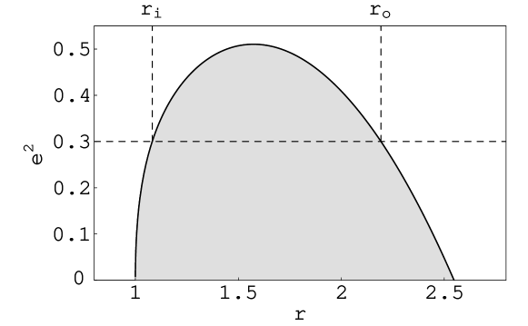
Figure 3: The function determining reality condition $D_{\rm z}(r;e)\geq 0$ for the radii at which the centrifugal force vanishes. Inside the shaded region, there is $D_{\rm z}(r;e)<0$, and the functions $a^{2}_{{\rm z}\pm}(r;e)$ are not defined there. The three remaining solutions of the equation $D_{\rm z}(r;e)=0$ are not presented here, being physically irrelevant (with $a^{2}<0$ or $e^{2}<0$).

The reality condition for $a^{2}_{{\rm z}\pm}(r;e)$ is

$$D_{\rm z}(r;e)\geq 0,$$ (44)

which can be treated easily considering $D_{\rm z}(r;e)$ as a quartic polynom in $e^{2}$. The results are given in Fig. 3. Detailed behaviour of the functions $a^{2}_{{\rm z}\pm}(r;e)$ will be determined in the next section, since it is closely related to embedding diagrams of the equatorial plane of the optical geometry.

4 Embedding diagrams of the optical geometry

Metric coefficients of the optical geometry of the Kerr–Newman spacetimes are, due to Eq. (4), given by the relations

$$\tilde{h}_{rr}=\frac{\tilde{h}_{\theta\theta}}{\Delta}=\frac{A}{\Delta^{2}},\quad\tilde{h}_{\phi\phi}=\frac{A^{2}}{\Delta\Sigma^{2}}\sin^{2}\theta.$$ (45)

In the equatorial plane they reduce to

$$\tilde{h}_{rr}(\theta={\textstyle\frac{1}{2}}\pi)=\frac{(r^{2}+a^{2})^{2}-a^{2}\Delta}{\Delta^{2}},$$

$$\tilde{h}_{\phi\phi}(\theta={\textstyle\frac{1}{2}}\pi)=\frac{\left[(r^{2}+a^{2})^{2}-a^{2}\Delta\right]^{2}}{r^{4}\Delta}.$$ (46)

The properties of the optical geometry related to the Kerr–Newman spacetimes can conveniently be represented by embedding of the equatorial (symmetry) plane into the 3-dimensional Euclidean space with line element expressed in the cylindrical coordinates ($\rho,z,\phi$) in the form

$${\rm d}\sigma^{2}={\rm d}\rho^{2}+\rho^{2}\,{\rm d}\phi+{\rm d}z^{2}.$$ (47)

The embedding diagram is characterised by the embedding formula $z=z(\rho)$ determining a surface in the Euclidean space with the line element

$${\rm d}\ell^{2}_{\rm(E)}=\left[1+\left(\frac{{\rm d}z}{{\rm d}\rho}\right)^{2}\right]{\rm d}\rho^{2}+\rho^{2}\,{\rm d}\phi^{2}$$ (48)

isometric to the 2-dimensional equatorial plane of the optical space determined by the line element

$${\rm d}\tilde{\ell}^{2}=\tilde{h}_{rr}\,{\rm d}r^{2}+\tilde{h}_{\phi\phi}\,{\rm d}\phi^{2}$$ (49)

with $\tilde{h}_{rr}$ and $\tilde{h}_{\phi\phi}$ given by (46).

The azimuthal coordinates can be identified, the radial coordinates are related as

$$\rho^{2}=\tilde{h}_{\phi\phi},$$ (50)

and the embedding formula is governed by the relation

$$\left(\frac{{\rm d}z}{{\rm d}\rho}\right)^{2}=\tilde{h}_{rr}\left(\frac{{\rm d}r}{{\rm d}\rho}\right)^{2}-1.$$ (51)

It is convenient to transfer the embedding formula into a parametric form $z(\rho)=z(r(\rho))$ with $r$ being the parameter. Then

$$\frac{{\rm d}z}{{\rm d}r}=\pm\sqrt{\frac{(r^{2}+a^{2})^{2}-a^{2}\Delta}{\Delta^{2}}-\left(\frac{{\rm d}\rho}{{\rm d}r}\right)^{2}}.$$ (52)

The sign in this formula is irrelevant, leading to isometric surfaces. Because

$$\frac{{\rm d}z}{{\rm d}\rho}=\frac{{\rm d}z}{{\rm d}r}\frac{{\rm d}r}{{\rm d}\rho},$$ (53)

the turning points of the embedding diagram, giving its throats and bellies, are determined by the condition ${\rm d}\rho/{\rm d}r=0$, where

$$\frac{{\rm d}\rho}{{\rm d}r} = \{r^{4}[r(r-3)+2e^{2}]+a^{2}[2e^{4}+e^{2}r(3r-7)+r^{2}(r^{2}-3r+6)]-$$ (54)

$$2a^{4}(r-e^{2})\}[r^{3}(r^{2}-2r+a^{2}+e^{2})^{3/2}].$$

By comparing Eqs (28) and (54) we can immediately see that turning points of the embedding diagrams are really located at the radii where the centrifugal force vanishes and changes sign. Thus, we can conclude that just this property of embeddings of the optical geometry of the vacuum spherically symmetric spacetimes (see [1, 10, 13]) survives in the Kerr–Newman spacetimes. However, photon circular orbits are displaced from the radii corresponding to the turning points of the embedding diagrams. Therefore, it is interesting to find the situations where the photon circular orbits lie within the regions of embeddability of the optical geometry.

4.1 Limits of embeddability

The embeddability condition $\left({\rm d}z/{\rm d}r\right)^{2}\geq 0$ (see (52)) implies the relation

$$E(r;a,e) = 4r^{11}-3(e^{2}+3)r^{10}+12(a^{2}+e^{2})r^{9}-$$ (55)

$$2(17a^{2}+5a^{2}e^{2}+2e^{4})r^{8}+4(9a^{2}+3a^{4}+12a^{2}e^{2})r^{7}-$$

$$(33a^{4}+66a^{2}e^{2}+11a^{4}e^{2}+17a^{2}e^{4})r^{6}+$$

$$4(9a^{4}+a^{6}+13a^{4}e^{2}+10a^{2}e^{4})r^{5}-$$

$$(36a^{4}+12a^{6}+78a^{4}e^{2}+4a^{6}e^{2}+21a^{4}e^{4}+8a^{2}e^{6})r^{4}+$$

$$2(12a^{6}+42a^{4}e^{2}+12a^{6}e^{2}+27a^{4}e^{4})r^{3}-$$

$$(4a^{8}+52a^{6}e^{2}+73a^{4}e^{4}+12a^{6}e^{4}+12a^{4}e^{6})r^{2}+$$

$$4(2a^{8}e^{2}+9a^{6}e^{4}+7a^{4}e^{6})r-$$

$$4(a^{8}e^{4}+2a^{6}e^{6}+a^{4}e^{8})\geq 0.$$

The function $E(r;a,e)$ can be considered as a polynom quartic both in $a^{2}$ and $e^{2}$. For $e^{2}=0$, the function $E(r;a)$ is still a polynom quartic in $a^{2}$ (see [15] for details). However, for $a^{2}=0$, the function $E(r;e)$ simplifies significantly, being only a polynom quadratic in $e^{2}$

$$E(r;e)=r^{8}[r^{2}(4r-9)+3r(4-r)e^{2}-4e^{4}];$$ (56)

its behaviour is discussed in [10]. For $a^{2}=e^{2}=0$ we arrive at the well-known Schwarzschild condition $r\geq\frac{9}{4}$.

The limits of embeddability are determined by the condition $E(r;a,e)=0$ which can be solved as a quartic equation in $a^{2}$. Let us denote the four solutions as $a^{2}_{{\rm e}k}(r;e)$, $k\in\{1,2,3,4\}$. Instead of giving long explicit expressions for the four solutions $a^{2}_{{\rm e}k}(r;e)$ we will treat them numerically and classify qualitatively; different types of their behaviour will be described. Of course, we naturally restrict our attention to physically relevant situations when $a^{2}\geq 0$ and $e^{2}\geq 0$.

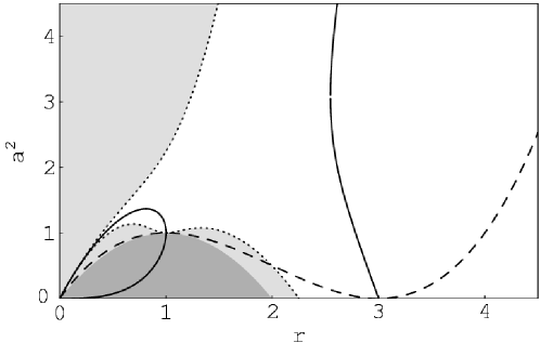
Figure 4: Square of the specific angular momentum of the Kerr backgrounds corresponding to the event horizons ($a^{2}_{\rm h}(r;e)$, the border between the dark gray dynamic area, in which the optical geometry is not defined, and the light gray non-embeddable area), photon circular orbits ($a^{2}_{\rm ph}(r;e)$, dashed curve), turning points of the embedding diagram ($a^{2}_{{\rm z}\pm}(r;e)$, solid curve), and embeddability region border ($a^{2}_{\rm e}(r;e)$, dotted curve enclosing the light gray area not embeddable into Euclidean space) are drawn as functions of the radius for fixed value $e^{2}=0$.

Recall that if $e^{2}=0$, the limits of embeddability are given by the solutions $a^{2}_{{\rm e}3}(r)$, $a^{2}_{{\rm e}4}(r)$ representing two branches, both reaching zero at $r=0$ (see Fig. 4). The upper branch ($a^{2}_{{\rm e}4}$) diverges for $r\rightarrow\infty$. The lower one ($a^{2}_{{\rm e}3}$) has a local minimum at $r=1$, where $a^{2}_{{\rm e}({\rm min})}=1$, and two local maxima, $a^{2}_{{\rm e}({\rm max},2)}=1.13540$ at $r=0.68947$, and $a^{2}_{{\rm e}({\rm max},1)}=1.07543$ at $r=1.33172$; its second zero point is located at $r=2.25$, corresponding to the Schwarzschild case [15].

If $e^{2}>0$, the limits of embeddability still consist of two branches. We can consider three qualitatively different situations.

4.1.1 Class Ea: $e^{2}\in(0,0.68950)$

The two branches are given by the solutions $a^{2}_{{\rm e}3}(r;e)$ and $a^{2}_{{\rm e}4}(r;e)$, again. Both the branches diverge at $r=e^{2}$. The upper branch ($a^{2}_{{\rm e}4}$) diverges also for $r\rightarrow\infty$, having a local minimum $a^{2}_{{\rm e}4({\rm min})}$ near $r=e^{2}$. The lower branch ($a^{2}_{{\rm e}3}$) has always a local minimum at $r=1$, where $a^{2}_{{\rm e}({\rm min})}=1-e^{2}$, corresponding to extreme black-hole states, and a local maximum $a^{2}_{{\rm e}({\rm max},1)}>1-e^{2}$ at $r>1$. Its zero point, corresponding to the Reissner–Nordström case, is determined by $E(r;e)=0$ (cf. Eq. (56)). It can also have a local minimum $a^{2}_{{\rm e}3({\rm min})}$ and a local maximum $a^{2}_{{\rm e}3({\rm max},2)}$ at $r<1$. Positions of $a^{2}_{{\rm e}4({\rm min})}$ and $a^{2}_{{\rm e}3({\rm min})}$ relative to the value $a^{2}=1-e^{2}$, and the relation between $a^{2}_{{\rm e}4({\rm min})}$ and $a^{2}_{{\rm e}3({\rm max},2)}$, or $a^{2}_{{\rm e}3({\rm max},1)}$, determine different members of embeddable regions of the Kerr–Newman black-hole and naked-singularity spacetimes. We can give the following subclassification of the spacetimes listed by the number of embeddable regions according to the values of the parameter $e^{2}$; for fixed $e^{2}$ from given interval, the numbers of the embeddable regions are given with the parameter $a^{2}$ growing:

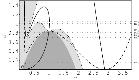
Figure 5: Square of the specific angular momentum of the Kerr–Newman backgrounds corresponding to the event horizons ($a^{2}_{\rm h}(r;e)$, between the dark gray dynamic area, in which the optical geometry is not defined, and the light gray non-embeddable area), photon circular orbits ($a^{2}_{\rm ph}(r;e)$, dashed curve), turning points of the embedding diagram ($a^{2}_{{\rm z}\pm}(r;e)$, solid curve), and embeddability region border ($a^{2}_{\rm e}(r;e)$, dotted curve enclosing the light gray area not embeddable into Euclidean space) are drawn as functions of the radius for fixed value $e^{2}=0.16$. This case covers all four types of black-hole embedding diagrams and the first three cases of naked-singularity diagrams. They are determined by the lines $a^{2}={\rm const}$, and depicted by the notation of the classification according to the properties of embedding diagrams (BH₁–BH₄, NS₁–NS₃). The dotted vertical line is common vertical asymptote of $a^{2}_{\rm ph}(r;e)$, $a^{2}_{{\rm c}\pm}(r;e)$, and $a^{2}_{\rm e}(r;e)$.

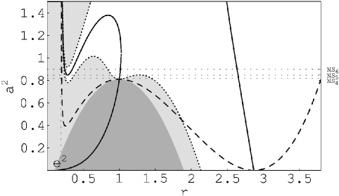
Figure 6: The functions $a^{2}_{\rm h}(r;e)$, $a^{2}_{\rm ph}(r;e)$, $a^{2}_{{\rm c}\pm}(r;e)$, and $a^{2}_{\rm e}(r;e)$ drawn for fixed value $e^{2}=0.19$. The naked-singularity classes NS₄–NS₆ are depicted.

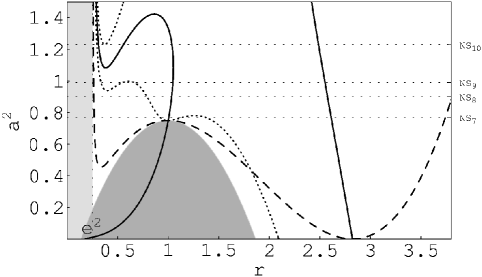
Figure 7: The functions $a^{2}_{\rm h}(r;e)$, $a^{2}_{\rm ph}(r;e)$, $a^{2}_{{\rm c}\pm}(r;e)$, and $a^{2}_{\rm e}(r;e)$ drawn for fixed value $e^{2}=0.25$. The naked-singularity classes NS₇–NS₁₀ are depicted.

Subclass	Interval of $e^{2}$	Black holes	Naked singularities
Ea1	$\langle 0,0.17230)$	$1,2,3$	$4,3,2$
Ea2	$\langle 0.17230,0.17906)$	$1,2$	$3,4,3,2$
Ea3	$\langle 0.17906,0.19749)$	$1,2$	$3,2,3,2$
Ea4	$\langle 0.19749,0.20670)$	1	$2,3,2,3,2$
Ea5	$\langle 0.20670,0.20794)$	1	$2,1,2,3,2$
Ea6	$\langle 0.20794,0.28961)$	1	$2,1,2,1,2$
Ea7	$\langle 0.28961,0.68950)$	1	$2,1,2$

Notice that in all of the subclasses Ea₁–Ea₇, both the branches of the limit of embeddability are defined at $r>e^{2}$. The behaviour of the embeddability limits in the subclasses Ea₁, Ea₃, and Ea₆ is illustrated in the Figs 5, 6, and 7, respectively.

4.1.2 Class Eb: $e^{2}\in(0.68950,2.205)$

The limits of embeddability have two branches. The upper one is determined by the solution $a^{2}_{{\rm e}4}(r;e)$. Again, it is well defined at $r>e^{2}$ only, diverges at $r=e^{2}$ and for $r\rightarrow\infty$, having a minimum near $r=e^{2}$. The lower branch is radically different from the class Ea. The solution $a^{2}_{{\rm e}3}(r;e)$ diverges at $r=e^{2}$ again, but it has a discontinuity, which is ‘filled up’ by various combinations of the solutions $a^{2}_{{\rm e}1}(r;e)$, $a^{2}_{{\rm e}2}(r;e)$, and $a^{2}_{{\rm e}4}(r;e)$. The combinations depend on the parameter $e^{2}$. However, it is not worth to discuss them explicitly because they have common basic properties. They have no local extrema, but two lobes—an external (upper) one, and an internal (lower) one. The internal lobe can enter the region of $r<e^{2}$ for $e^{2}$ high enough; for $e^{2}>1$, the internal lobe is shifted to the physically irrelevant region, where $a^{2}<0$. If $e^{2}<1$, the solution $a^{2}_{{\rm e}3}(r;e)$ has a local minimum at $r=1$, with $a^{2}=1-e^{2}$ corresponding to an extreme black-hole, and a local maximum $a^{2}_{{\rm e}({\rm max},1)}>1-e^{2}$ at $r>1$; for $e^{2}=1$ these local extrema coalesce at $r=1$, $a^{2}_{{\rm e}3}=0$. Therefore, the subclassification according to the number of embeddable regions can be given in the following simple way (with $a^{2}$ growing):

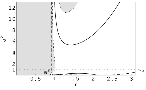
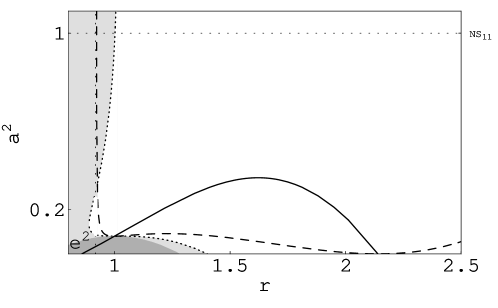
Figure 8: The functions $a^{2}_{\rm h}(r;e)$, $a^{2}_{\rm ph}(r;e)$, $a^{2}_{{\rm c}\pm}(r;e)$, and $a^{2}_{\rm e}(r;e)$ drawn for fixed value $e^{2}=0.92$. Contrary to the preceding cases, there exist lobes of $a^{2}_{\rm e}(r;e)$, and $a^{2}_{{\rm z}\pm}(r;e)$ is defined for all $r\geq e^{2}$. However, there exist an interval of the parameter $a^{2}$ corresponding to naked-singularity spacetimes, at which no turning points appear on the embedding diagrams—these are the NS₁₁-spacetimes.

Subclass	Interval of $e^{2}$	Black holes	Naked singularities
Eb1	$\langle 0.68950,1)$	1	$2,1,2$
Eb2	$\langle 1,2.205)$	none	$1,2$

An example of subclass Eb₁ can be seen in Fig. 8.

4.1.3 Class Ec: $e^{2}\in(2.205,\infty)$

The limits of embeddability $a^{2}_{{\rm e}}(r;e)$ have two branches, again. However, now both the branches are determined by the solution $a^{2}_{{\rm e}4}(r;e)$. The first branch is defined at $r>e^{2}$, diverges at $r=e^{2}$ and for $r\rightarrow\infty$, having a local minimum near $r=e^{2}$. The second branch is relevant from some $r<e^{2}$, where $a^{2}_{{\rm e}4}=0$, and it diverges at $r=e^{2}$, having no local extreme. The subclassification according to the number of embeddable regions is simply given just by one case (with $a^{2}$ growing):

Subclass	Interval of $e^{2}$	Black holes	Naked singularities
Ec1	$\langle 2.205,\infty)$	none	$1,2$

Note that in situations which are necessary in order to construct typical embedding diagrams, the curves $a^{2}_{\rm e}(r;e)$ are given explicitly (see Figs 5–8). The behaviour of the embeddability limits of the class Ec is not illustrated because they give no qualitatively different kind of embedding diagrams.

4.2 Turning points of the embedding diagrams

The embeddable regions are characterised by the number of radii where the embedding diagrams have turning points, or, equivalently, where the centrifugal force determined by (28) vanishes. Therefore, the turning points of the diagrams are governed by the functions $a^{2}_{{\rm z}\pm}(r;e)$ determined by (42) and (43). We shall discuss the behaviour of these functions and introduce a corresponding classification of the Kerr–Newman backgrounds (relative to their parameter $e^{2}$) according to the number of turning points of the embedding diagrams of their optical geometry.

It follows from the reality condition (44) (see also Fig. 3) that for $e^{2}<e^{2}_{\rm cr}=0.51033$ the functions $a^{2}_{{\rm c}\pm}(r;e)$ are not defined between the radii $r_{\rm i}(e)$, $r_{\rm o}(e)$, i.e., inside the shaded region in Fig. 3. If $e^{2}=0$ (see Fig. 4), there is $a^{2}_{{\rm c}\pm}(r=0)=0$, and $a^{2}_{{\rm c}-}(r=3)=0$. The part of $a^{2}_{{\rm c}-}(r,0)$ starting at $r=0$ is located in the region between the horizons, and, therefore, is physically irrelevant; a local maximum of $a^{2}_{{\rm z}+}(r)$ is located at $r_{\rm(max,1)}=0.81159$ with $a^{2}_{{\rm z}+{\rm(max,1)}}=1.36668$; $a^{2}_{{\rm c}+}(r)$ and $a^{2}_{{\rm z}-}(r)$ coincide at $r=1$ with $a^{2}=1$, corresponding to an extreme black-hole (see [15]).

For $e^{2}>0$, we can separate qualitatively different classes of the behaviour of $a^{2}_{{\rm z}\pm}(r;e)$ in the following way.

4.2.1 Class Ta: $e^{2}\in(0,0.51033)$

According to the reality condition (44), the functions $a^{2}_{{\rm z}\pm}(r;e)$ are defined at $r\leq r_{\rm i}(e)$, and $r\geq r_{\rm o}(e)$. For $r=r_{\rm i}(e)$, $r=r_{\rm o}(e)$, there is $a^{2}_{{\rm z}+}=a^{2}_{{\rm c}-}$. At $r>r_{\rm o}(e)$, the function $a^{2}_{{\rm z}-}(r;e)$ has a zero point, while $a^{2}_{{\rm z}+}(r;e)$ diverges for $r\rightarrow+\infty$. The functions $a^{2}_{{\rm c}\pm}(r;e)$ have no extrema at $r>r_{\rm o}(e)$. At $r<r_{\rm i}(e)$, the function $a^{2}_{{\rm z}-}(r;e)$ grows from its zero point up to $r=r_{\rm i}(e)$, it is physically irrelevant up to $r=1$, where $a^{2}_{{\rm z}-}(r=1,e)=1-e^{2}$. The function $a^{2}_{{\rm c}+}(r;e)$ diverges at $r=e^{2}$; it has a local minimum $a^{2}_{{\rm c}+{\rm(min)}}(e)$ at $r_{{\rm z}({\rm min})}(e)$ and a local maximum $a^{2}_{{\rm c}+({\rm max})}(e)$ at $r_{{\rm c}({\rm max})}(e)$; of course $r_{{\rm z}({\rm min})}<r_{{\rm z}({\rm max})}<r_{\rm i}$. Relating $a^{2}_{{\rm z}+({\rm min})}(e)$ to $a^{2}=1-e^{2}$ enables us to give the classification of black-hole and naked-singularity backgrounds according to the number of turning points of the embedding diagrams. (A classification of these backgrounds relating the number of turning points and the number of embeddable regions can be realized by relating $a^{2}_{e4({\rm min})}$ with $a^{2}_{{\rm c}+({\rm max})}$, and $a^{2}_{e3({\rm max},2)}$ with $a^{2}_{{\rm z}+({\rm min})}$.)

The subclassification according to the number of turning points can be given in the following way (with $a^{2}$ growing):

Subclass	Interval of $e^{2}$	Black holes	Naked singularities
Ta1	$\langle 0,0.18275)$	$1,3$	$4,2$
Ta2	$\langle 0.18275,0.51033)$	1	$2,4,2$

Examples of subclasses Ta₁ and Ta₂ are given in Figs 5 and 6 or 7, respectively.

4.2.2 Class Tb: $e^{2}\in(0.51033,1.125)$

If $e^{2}$ equals to the critical value $e^{2}_{\rm cr}=0.51033$, $r_{\rm i}(e)=r_{\rm o}(e)$, and the two branches of $a^{2}_{{\rm c}+}$ and $a^{2}_{{\rm z}-}$ coalesce. For $e^{2}>e^{2}_{\rm cr}$, the reality condition (44) is satisfied everywhere, and $a^{2}_{{\rm c}-}(r;e)$, and $a^{2}_{{\rm z}+}(r;e)$ give two separated branches of the turning points. The function $a^{2}_{{\rm z}-}(r;e)$ determining the lower branch is physically irrelevant at $r<1$, being located between the horizons, and it has a local maximum $a^{2}_{{\rm z}-({\rm max})}(e)$ at $r>1$. The function $a^{2}_{{\rm z}+}(r;e)$ giving the upper branch diverges at $r=e^{2}$ and for $r\rightarrow\infty$, and it can have a local minimum $a^{2}_{{\rm z}+({\rm min})}$ near $r=e^{2}$, or two local minima $a^{2}_{{\rm z}+({\rm min},1)}$, $a^{2}_{{\rm z}+({\rm min},2)}$ and a local maximum $a^{2}_{{\rm c}+({\rm max})}$ between them. Now, the subclassification according to the number of turning points can be given as follows (with $a^{2}$ growing):

Subclass	Interval of $e^{2}$	Black holes	Naked singularities
Tb1	$\langle 0.51033,0.52480)$	1	$2,0,2,4,2$
Tb2	$\langle 0.52480,1)$	1	$2,0,2$
Tb3	$\langle 1,1.125)$	none	$2,0,2$

An example of subclass Tb₂ is given in Fig. 8.

4.2.3 Class Tc: $e^{2}\in(1.125,\infty)$

Now, the function $a^{2}_{{\rm c}-}(r;e)$ is irrelevant, being shifted to negative values completely. The function $a^{2}_{{\rm c}+}(r;e)$ behaves in the same way as that of the subclass Tb₃. The classification according to the number of turning point is the following:

Subclass	Interval of $e^{2}$	Black holes	Naked singularities
Tc1	$\langle 1.125,\infty)$	none	$0,2$

We can conclude that outside the outer black-hole horizon, there is always an embeddable region, covering exterior of the black hole except a small part in the vicinity of the outer horizon, and containing just one turning point corresponding to a throat of the embedding diagram. So, the situation is the same as for Schwarzschild, Reissner–Nordström, and Kerr black holes. On the other hand, under the inner horizon, the embeddable region contains no turning point, or two turning points corresponding to a throat and a belly; we do not consider the case of coalescing of the two turning points in an inflex point separately.

For the naked-singularity backgrounds, the situation is much more complex, including various possibilities of the number of the embeddable regions and the turning points of the diagrams. There are a lot of cases that cannot appear with Kerr naked singularities [15]. As examples, let us mention one region with four turning points, and one region with no turning point. Again, in situations which are necessary in order to determine behaviour of typical embedding diagrams, the curves $a^{2}_{{\rm z}\pm}(r;e)$ are given explicitly (see Figs 5–8).

4.3 Embeddability of photon circular orbits

The motion of a photon in the equatorial plane of Kerr–Newman spacetimes is determined by the function (see, e.g., [16])

$$R(r;a,e,E,\Phi)=[Er^{2}-a(\Phi-aE)]^{2}-\Delta(\Phi-aE)^{2},$$ (57)

where $E$ is the covariant energy of the photon, and $\Phi$ is its axial angular momentum. For photon circular orbits the conditions

$$R=0,\quad\frac{\partial R}{\partial r}=0$$ (58)

must be satisfied simultaneously. The equatorial photon motion is fully governed by the impact parameter

$$\ell=\frac{\Phi}{E}.$$ (59)

It follows from the conditions (58) that the radii of photon circular orbits are determined by the equation

$$r^{2}-3r+2a^{2}+2e^{2}\pm 2a\Delta^{1/2}=0;$$ (60)

the corresponding impact parameter is given by the relation

$$\ell=-\frac{a(r^{2}+3r-2e^{2})}{r^{2}-3r+2e^{2}}.$$ (61)

Equivalently, the radii of photon circular orbits can be determined by

$$a^{2}=a^{2}_{\rm ph}(r;e)=\frac{(r^{2}-3r+2e^{2})^{2}}{4(r-e^{2})}.$$ (62)

Clearly, the circular orbits must be located at

$$r\geq e^{2}.$$ (63)

The zero points of $a^{2}_{\rm ph}(r;e)$ are located at radii

$$r_{1}(e)={\textstyle\frac{1}{2}}[3-(9-8e^{2})^{1/2}],\quad r_{2}(e)={\textstyle\frac{1}{2}}[3+(9-8e^{2})^{1/2}],$$ (64)

giving photon circular orbits of Reissner–Nordström spacetimes. The extrema of $a^{2}_{\rm ph}(r;e)$ are located at the zero points $r_{1}(e)$, $r_{2}(e)$ (if $e^{2}<\textstyle{\frac{9}{8}}$), at $r=1$ (if $e^{2}<1$) and at

$$r={\textstyle\frac{4}{3}}e^{2},$$ (65)

where a minimum exists for $e^{2}<\frac{3}{4}$, a maximum for $\frac{3}{4}<e^{2}<\frac{9}{8}$, and a minimum for $e^{2}\geq\frac{9}{8}$. At $r=\frac{4}{3}e^{2}$, the value of $a^{2}_{\rm ph}(r;e)$ is given by the function

$$a^{2}_{\rm ex}(e)={\textstyle\frac{1}{27}}e^{2}(8e^{2}-9)^{2}.$$ (66)

The function $a^{2}_{\rm ex}(e)$ determines boundary between Kerr–Newman spacetimes containing different numbers of photon circular orbits. If $e^{2}<\frac{3}{4}$, there can be 2 or 4 circular orbits in the black-hole spacetimes and 2 orbits in naked-singularity spacetimes. If $\frac{3}{4}<e^{2}<1$, there are 2 circular orbits in black-hole and 2 or 4 orbits in naked-singularity spacetimes. For the naked-singularity spacetimes with $1<e^{2}<\frac{9}{8}$, there are 2 or 4 orbits; if $e^{2}>\frac{9}{8}$, there are 0 or 2 orbits.

Class Pa: $e^{2}=0.16$

Class Pc: $e^{2}=0.78$

Class Pe: $e^{2}=0.81$

Class Pg: $e^{2}=0.86$

Class Pi: $e^{2}=1.3$

Class Pb: $e^{2}=0.35$

Class Pd: $e^{2}=0.804$

Class Pf: $e^{2}=0.822$

Class Ph: $e^{2}=1.05$

Class Pj: $e^{2}=2.3$

Figure 9: Embeddability of photon circular orbits in the embedding diagrams of the optical geometry. It is determined by the relations of the curves $a^{2}_{\rm e}(r;e)$ (dotted lines) giving the limits of embeddability, and $a^{2}_{\rm ph}(r;e)$ (dashed lines) giving radii of the photon circular orbits. We present all of the typical situations representing the classes Pa–Pj, restricting our attention on the relevant parts of the functions $a^{2}_{\rm e}(r;e)$ and $a^{2}_{\rm ph}(r;e)$. Note that the circular orbits under the inner black-hole horizon are always outside the embeddable regions.

Figure 10: Classification of the Kerr–Newman spacetimes according to embeddability of photon circular orbits. The solid lines separate regions of the parameter $a^{2}$-$e^{2}$ corresponding to spacetimes containing different numbers of the circular orbits; the bold solid straight line correspond to extreme black-hole spacetimes. The dashed line separates regions of the parameter space with different numbers of the embeddable circular orbits. The S-shaped solid curve is given by Eq. (66). The corresponding region of the parameter space are depicted by pairs of digits, the first one expressing number of the circular orbits, the second one (in parentheses) the number of the embeddable orbits. (a) the global view of the classification, (b,c) details of some narrow regions located in the vicinity of the extreme black-hole states, where the structure is rather complicated.

In the case of extreme black holes ($a^{2}+e^{2}=1$), the radii of photon circular orbits and corresponding values of the impact parameter are

$$\begin{array}[]{ll}r=1,&\quad\ell=a+1/a,\\ r=2-2a,&\quad\ell=4-3a,\\ r=2+2a,&\quad\ell=-(4+3a),\end{array}$$ (67)

The counterrotating orbit at $r=2+2a$ is always located above the horizon. The corotating orbit at $r=2-2a$ is located above the horizon if $e^{2}>\frac{3}{4}$, and under the horizon if $e^{2}<\frac{3}{4}$. There are two orbits at $r=1$ if $e^{2}<\frac{3}{4}$, but no circular orbit at $r=1$, if $e^{2}>\frac{3}{4}$ (see [16] for details).

Now, we shall discuss in which cases the photon circular orbits enter the regions of embeddability. Radii of the photon circular orbits are determined by the function $a^{2}_{\rm ph}(r;e)$ given by Eq. (62). The embeddability of these orbits must be determined by a numerical procedure. Note that, generally, the function $a^{2}_{{\rm z}-}(r;e)$ has common points with $a^{2}_{\rm ph}(r;e)$ at its zero points (if $e^{2}<\frac{9}{8}$), and at $r=1$ (if $e^{2}<1$).

The classification of the Kerr–Newman spacetimes according to the embeddability of the photon circular orbits can be again given in a simple way. In the presented classification scheme related to the parameter $e^{2}$, the first digit gives the number of circular orbits, the digits in parentheses determine changes of the number of embeddable circular orbits, with parameter $a^{2}$ growing. Note that the circular orbits under the inner horizon are always outside the embeddable regions:

Class	Interval of $e^{2}$	Black holes	Naked singularities
Pa	$\langle 0,0.23083)$	$2(2),4(2,1)$	2(1)
Pb	$\langle 0.23083,\frac{3}{4})$	$2(2,1),4(1)$	2(1)
Pc	$\langle\frac{3}{4},0.80115)$	$2(2,1)$	$4(1),2(1)$
Pd	$\langle 0.80115,0.80797)$	2(2)	$4(2,1),2(1)$
Pe	$\langle 0.80797,0.82040)$	2(2)	$4(2,3),2(1)$
Pf	$\langle 0.82040,0.82488)$	2(2)	$4(4,3),2(1)$
Pg	$\langle 0.82488,1)$	2(2)	$4(4),2(2,1)$
Ph	$\langle 1,\frac{9}{8})$	none	$4(4),2(2,1)$
Pi	$\langle\frac{9}{8},1.70233)$	none	$0(0),2(2,1)$
Pj	$\langle 1.70233,\infty)$	none	$0(0),2(2)$

The embeddability of the photon circular orbits can be easily read out from the sequence of figures (Fig. 9) representing the classification given above.

Details of the classification, i.e., distribution in the parameter space of the Kerr–Newman backgrounds, must be determined by a numerical procedure. The results are presented in Fig. 10. The regions of the parameter plane $a^{2}$-$e^{2}$ are denoted by two digits. The first one gives the number of photon circular orbits in the corresponding background, the second one (in parentheses) gives the number of embeddable orbits.

4.4 Construction of the embedding diagrams

The relevant properties of the embedding diagrams are determined by the functions $a^{2}_{\rm e}(r;e)$ and $a^{2}_{\rm z}(r;e)$ governing embeddable parts of the optical reference geometry and turning points of the diagrams. We shall present a classification of the Kerr–Newman spacetimes according to the number of the embeddable regions, and the number of their turning points. All cases of the classification will be represented by a typical embedding diagram. Inspecting all of the types of the behaviour of functions $a^{2}_{{\rm c}\pm}(r;e)$ (given by classes Ta–Tc and their subclasses), we find that there are 4 cases of the behaviour of the embeddings for the black-hole spacetimes, and 11 cases for the naked-singularity spacetimes. A complete list of typical embeddings will be given by using behaviour of the characteristic functions $a^{2}_{\rm e}(r;e)$ and $a^{2}_{\rm z}(r;e)$ for some typical values of the parameter $e^{2}$—see Figs 5–8, where the functions $a^{2}_{\rm h}(r;e)$ and $a^{2}_{\rm ph}(r;e)$ are included for completeness. In order to obtain all of the 15 types of the embedding diagrams, it is necessary to consider at least four values of the parameter $e^{2}$ belonging subsequently to the subclasses Ea₁ ($e^{2}=0.16$), Ea₃ ($e^{2}=0.19$), Ea₆ ($e^{2}=0.25$), Eb₁ ($e^{2}=0.92$) of the classification according to the number of embeddable regions, discussed above. The behaviour of $a^{2}_{\rm c}(r;e)$ for these four values of $e^{2}$ enables us to present a complete list of typical embedding diagrams. The classes will be denoted successively with growing parameter $a^{2}$ for each fixed $e^{2}$.

In the regions of the optical geometry where the embeddability condition $E(r;a,e)\geq 0$ is satisfied, the embedding diagram can be constructed for a fixed parameter $a$ by integrating the parametrically expressed embedding formula $z(r)$ (cf. Eq. (52)), and transferring it into the final form $z(\rho)$ by an appropriate numerical procedure using (50). In all the typical diagrams also photon circular orbits are illustrated, if they enter the embeddable regions. (Of course, the presented diagrams do not cover all of the possibilities for the embeddability of photon circular orbits.)

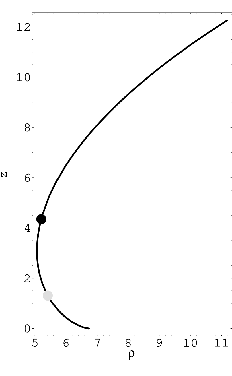
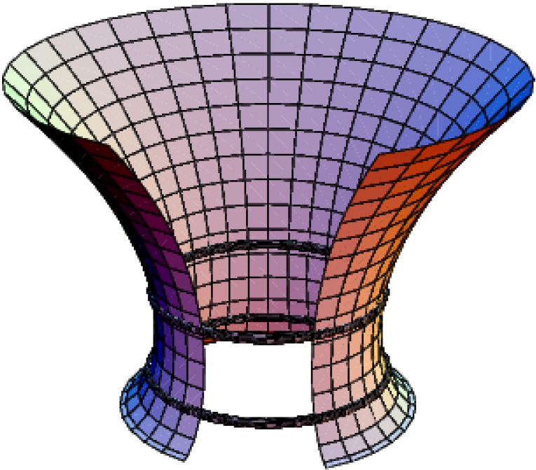
Figure 11: Embedding diagram of the Kerr–Newman black holes of the type BH₁, constructed for $a^{2}=0.16$, $e^{2}=0.16$. The rings in the 3D diagram represent photon circular orbits. Both corotating (gray spot in 2D diagram) and counterrotating (black spot in 2D diagram) are displaced from the throat of the diagram, where the centrifugal force vanishes. This is a general property of the rotating backgrounds.

(a)

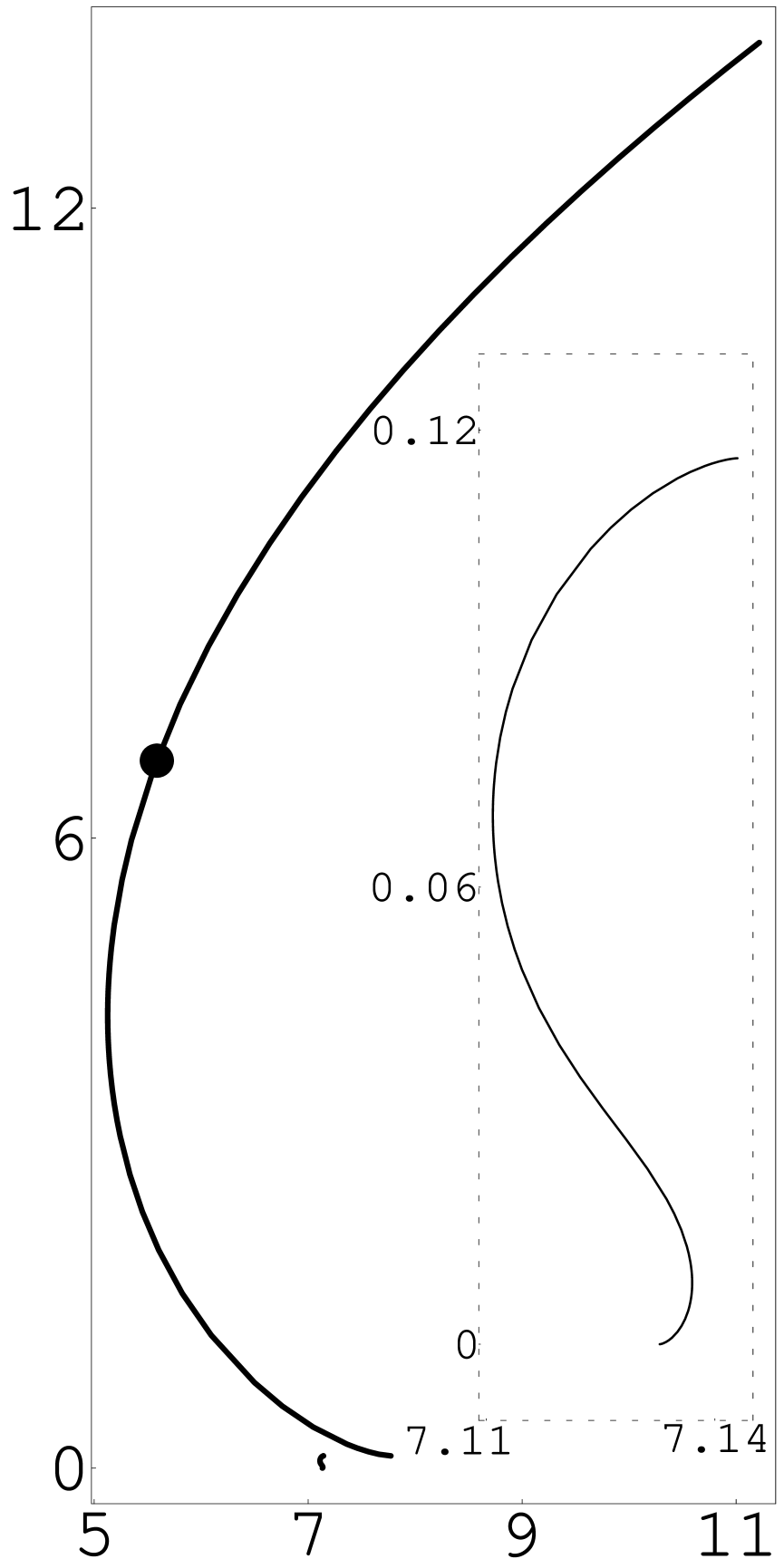
(b)

(c)

Figure 12: Embedding diagrams of the black holes classes BH₂–BH₄. (a) Class BH₂ ($a^{2}=0.7$, $e^{2}=0.16$); (b) class BH₃ ($a^{2}=0.75$, $e^{2}=0.16$); (c) class BH₄ ($a^{2}=0.81$, $e^{2}=0.16$).

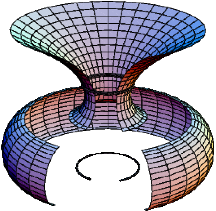
Figure 13: Embedding diagram of the NS₁ type, constructed for $a^{2}=0.86$, $e^{2}=0.16$.

(a)

(b)

(c)

(d)

(e)

(f)

(g)

(h)

(i)

(j)

Figure 14: Embedding diagrams of the types (a) NS₂ ($a^{2}=1$, $e^{2}=0.16$), (b) NS₃ ($a^{2}=1.05$, $e^{2}=0.16$), (c) NS₄ ($a^{2}=0.82$, $e^{2}=0.19$), (d) NS₅ ($a^{2}=0.847$, $e^{2}=0.19$), (e) NS₆ ($a^{2}=0.9$, $e^{2}=0.19$), (f) NS₇ ($a^{2}=0.77$, $e^{2}=0.25$), (g) NS₈ ($a^{2}=0.9$, $e^{2}=0.25$), (h) NS₉ ($a^{2}=0.99$, $e^{2}=0.25$), (i) NS₁₀ ($a^{2}=1.23$, $e^{2}=0.25$), and (j) NS₁₁ ($a^{2}=1$, $e^{2}=0.9$).

All of the black-hole diagrams are determined by Fig. 5. In order to cover all of the naked-singularity diagrams all Figs 5–8 have to be used. The typical diagrams are represented in Figs 11 and 12 for the black-hole spacetimes, and in Figs 13 and 14 for the naked-singularity spacetimes. We do not explicitly consider the cases corresponding to situations when extrema of $a^{2}_{\rm e}(r;e)$ coincide in an inflex point as they can be discussed in a straightforward manner.

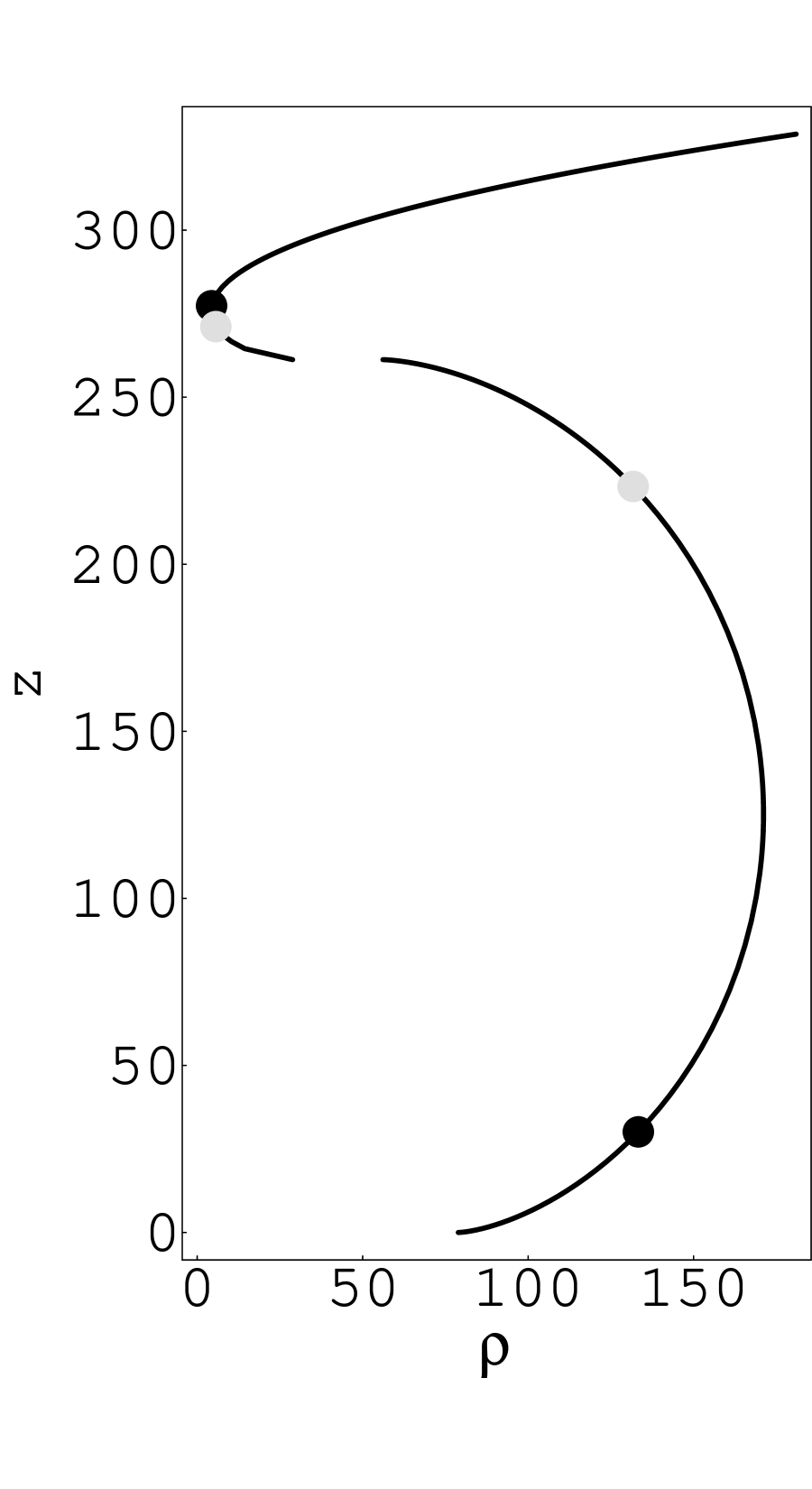
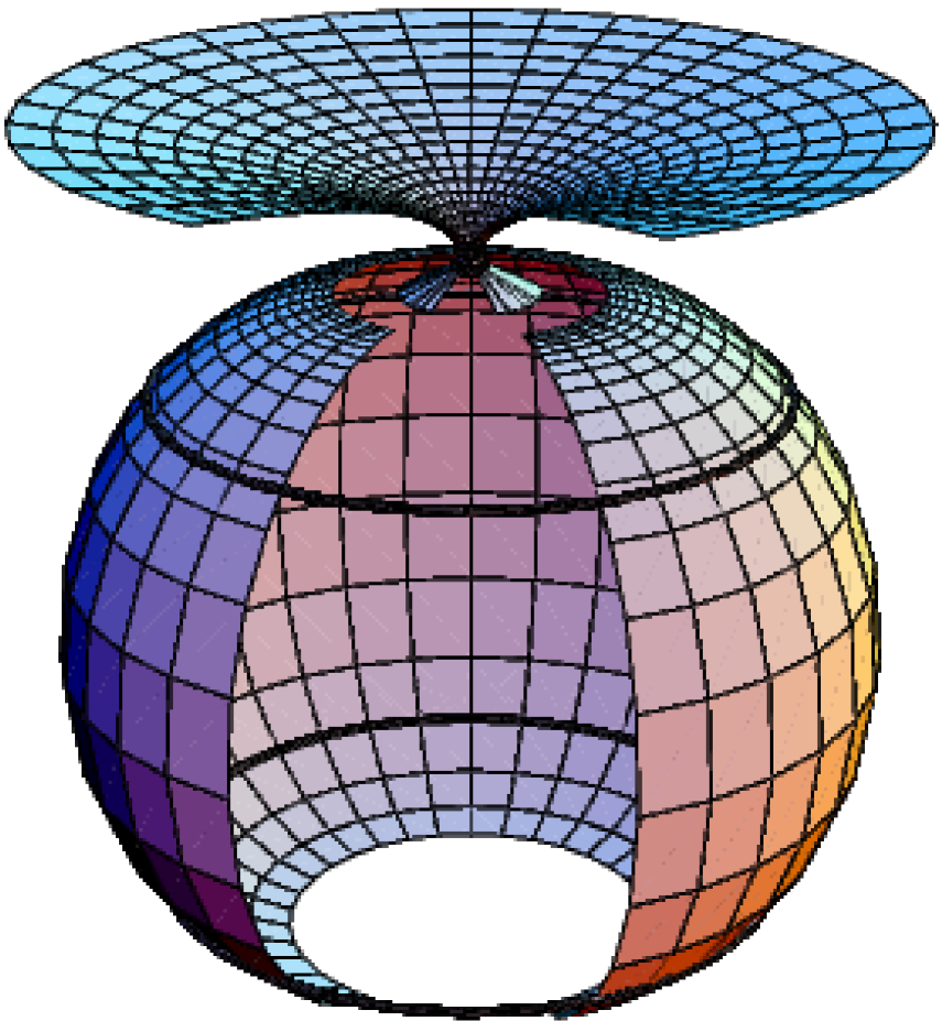
Figure 15: Embedding diagrams of the NS₇ type, constructed for $a^{2}=0.10005$, $e^{2}=0.9$. The diagram is separated into two regions having one throat and one belly. All four photon circular orbits find themselves in the embeddable region. In each region, one corotating orbit (gray spots) and one counterrotating one (black spots) exist.

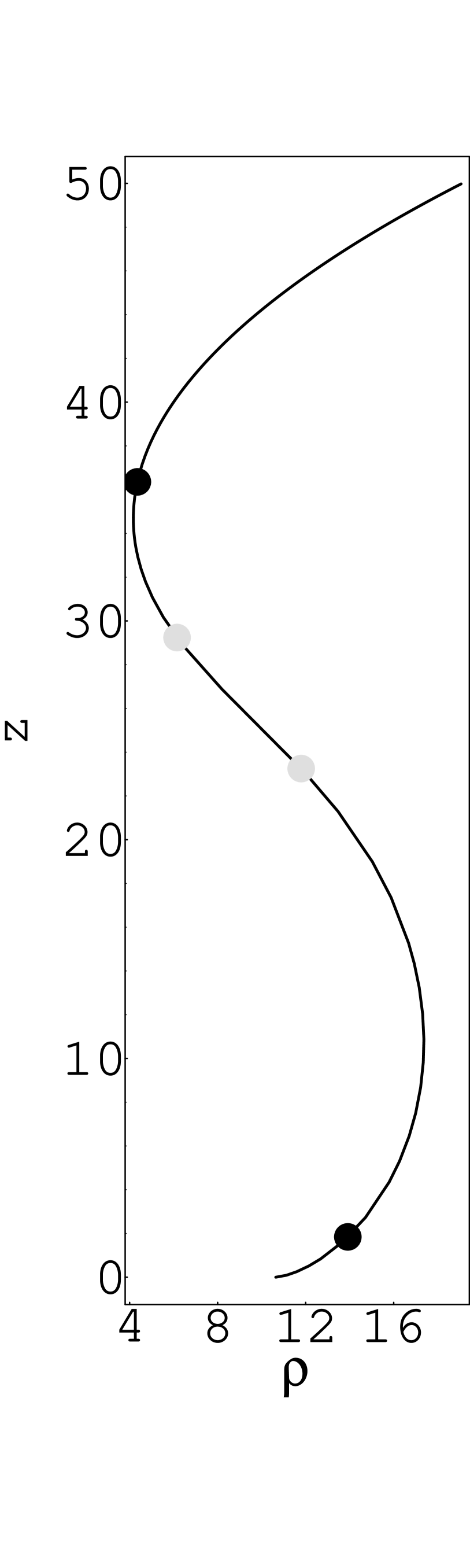
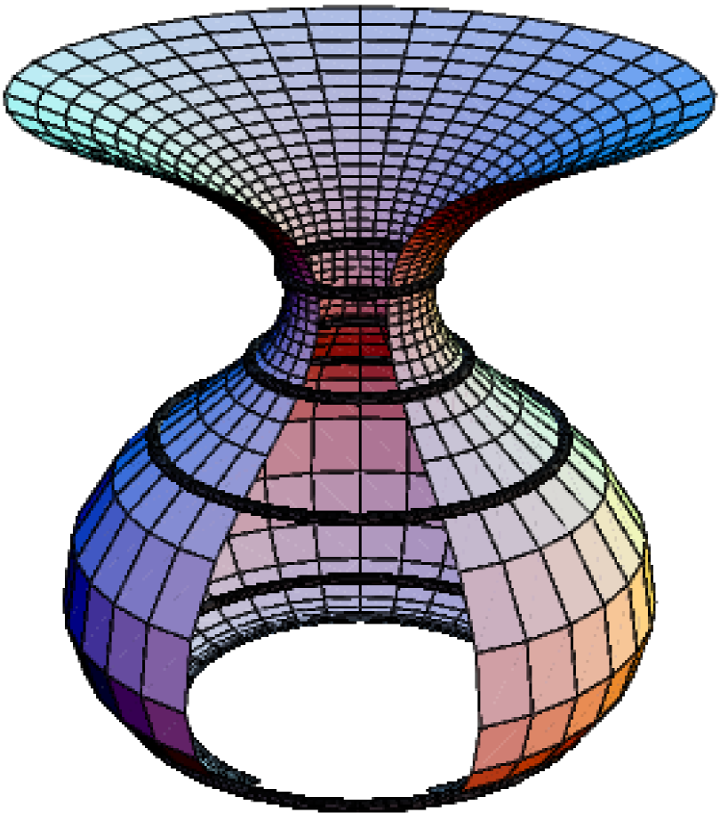
Figure 16: Embedding diagrams of the NS₈ type, constructed for $a^{2}=0.105$, $e^{2}=0.9$. The diagram is simply connected having one throat and belly. All four photon circular orbits find themselves in the embeddable region. The corotating and counterrotating circular photon orbits are displayed as gray and black spots, respectively.

The embeddability of photon circular orbits can be systematically discussed by using Figs 9 and 10, and behaviour of $a^{2}_{\rm e}(r;e)$ and $a^{2}_{\rm ph}(r;e)$ in related situations. We shall drop off the discussion here, we only explicitly mention two interesting cases of naked-singularity spacetimes containing four photon circular orbits all of which are located in the embeddable parts of the optical geometry instead. (Note that such a situation cannot occur in Kerr backgrounds.) In the first case ($a^{2}=0.10005$, $e^{2}=0.9$), there are two separated parts of the diagram, both containing two of the circular orbits (see Fig. 15), in the second case ($a^{2}=0.105$, $e^{2}=0.9$), there is only one region of embeddability containing all of the circular orbits (see Fig. 16). In both cases, the embedding diagrams necessarily have a throat and a belly.

4.5 The classification

The following classification will be made according to the properties of the embedding diagrams. The Kerr–Newman spacetimes are characterised by the number of embeddable regions of the optical geometry, and by the number of turning points at these regions, given successively for the regions with descending radial coordinate of the geometry (which are presented in parentheses). Therefore, the classification can be given in the following way:

BHs	NSs	NSs	NSs
BH1: $1(1)$	NS1: $4(1,1,1,1)$	NS5: $3(1,1,2)$	NS9:0 $2(2,0)$
BH2: $2(1,0)$	NS2: $3(2,1,1)$	NS6: $2(2,2)$	NS10: $1(4)$
BH3: $2(1,2)$	NS3: $2(3,1)$	NS7: $2(1,1)$	NS11: $1(0)$
BH4: $3(1,1,1)$	NS4: $3(1,1,0)$	NS8: $1(2)$

Figure 17: Classification of the Kerr–Newman spacetimes according to properties of the embedding diagrams. The solid lines separate spacetimes with different numbers of embeddable regions, the dashed lines separate spacetimes with different numbers of turning points (throats and bellies, in other words), at which the centrifugal force vanishes. The parameter plane $a^{2}$-$e^{2}$ is divided into regions corresponding to types BH₁–BH₄ and NS₁–NS₁₁. The central part marked by dotted rectangle is zoomed in the lower graph.

The parameter space of the Kerr–Newman spacetimes can be separated into regions corresponding to the classes BH₁–BH₄, and NS₁–NS₁₁ by a numerical code expressing the extreme points of the functions $a^{2}_{\rm e}(r;e)$ and $a^{2}_{\rm c}(r;e)$ as functions of $e^{2}$. Results of the numerical code are presented in Fig. 17, which represents the classification completely.

5 Concluding remarks

In the rotating black-hole and naked-singularity backgrounds, the embedding diagrams of the optical reference geometry reflect immediately just one important property of the inertial forces related to a test-particle circular motion. Namely, the turning points of the embedding diagrams occur just at radii where the centrifugal force vanishes and reverses sign, independently on the velocity of the motion. However, contrary to the spherically symmetric black-hole and naked-singularity backgrounds, in the rotating backgrounds radii of the photon circular orbits do not coincide with the radii of vanishing centrifugal force, and, moreover, in a variety of Kerr–Newman backgrounds, some of these orbits even are not located in the the regions of the optical geometry that are embeddable into the 3-dimensional Euclidean space.

The properties of the embedding diagrams have been discussed, and a classification scheme of the Kerr–Newman backgrounds reflecting the number of embeddable regions, and the number of turning points of these regions, was presented. The ring singularity in all of the rotating backgrounds, and the horizons of the black-hole backgrounds, are always located outside the embeddable regions. Further, embeddability of regions containing the photon circular orbit has been established.

The presence of a nonzero charge parameter $e$ in the Kerr–Newman backgrounds enriches significantly the variety of the embedding diagrams in comparison with the case of pure Kerr backgrounds [15].

For the black-hole backgrounds, there is just one embeddable region outside the outer horizon, containing just one throat. However, under the inner horizon, there can be two, one, or no embeddable regions. They can have a throat and a belly. Above the outer horizon, the outermost, counterrotating photon circular orbit is always embeddable, while the inner, corotating one is embeddable in backgrounds with sufficiently small specific angular momentum, but non-embeddable in the other ones. On the other hand, the photon circular orbits existing under the inner horizon are always located in the non-embeddable regions.

For the naked-singularity backgrounds, the variety of possible embedding diagrams is much more complex and can be directly read out from Figs 13–14. Let us point out the most important phenomena. There can exist diagrams consisting from four separated regions, or, oppositely, simply connected diagrams, having two throats and two bellies. On the other hand, there are also diagrams having no turning point. Moreover, in some naked-singularity backgrounds containing four photon circular orbits, all of the orbits are located in the embeddable regions—such situation is impossible in the black-hole backgrounds.

The embedding diagrams of the optical geometry give an important tool of visualisation and clarifying of the dynamical behaviour of test particles moving along equatorial circular orbits, by imagining that the motion is constrained on the surface $z(\rho)$ [10]. The shape of the surface $z(\rho)$ is directly related to the centrifugal acceleration. Within the rising portions of the embedding diagram, the centrifugal acceleration points towards increasing values of $r$, and the dynamics of test particles has essentially Newtonian character. However, in the descending portions of the embedding diagrams, the centrifugal acceleration has a radically non-Newtonian character, as it points towards decreasing values of $r$. Such a kind of behaviour appears where the diagrams have a throat or a belly. At the turning points of the diagram, the centrifugal acceleration vanishes and changes its sign, i.e., ${\rm d}r/{\rm d}\rho={\rm d}z/{\rm d}\rho=0$.

We can understand this connection of the centrifugal force and the embedding of the optical space in terms of the radius of gyration representing rotational properties of rigid bodies. In Newtonian mechanics, it is defined as the radius $\tilde{R}$ of the circular orbit on which a point-like particle having the same mass $M$ and angular velocity $\Omega$ as a rigid body would have the same angular momentum $J$:

$$J=M\tilde{R}^{2}\Omega.$$ (68)

Defining a specific angular momentum $\ell=J/M$, we obtain

$$\tilde{R}=\sqrt{\frac{\ell}{\Omega}}.$$ (69)

For a point-like particle moving on $r={\rm const}$, there is $\tilde{R}=r$.

In general relativity, the radius of a circle can be given by two standard ways—namely as the circumferential radius, and as the proper radial distance. A third way can be given by generalising Eq. (69) for a point particle moving along $r={\rm const}$; we use $\ell=L/E$, where $L$ is the angular momentum of the particle, and $E$ is its energy. [In stationary spacetimes, the angular velocity have to be related to the family of locally non-rotating observers, cf. Eq. (23).] In Newtonian theory, these three definitions of radius issue identical results, however, in general relativity they are distinct. The radius of gyration $\tilde{R}$ is convenient for discussing the dynamical effects of rotation; the direction of increase of $\tilde{R}$ defines local outward direction of these effects. The surfaces $\tilde{R}={\rm const}$, called von Zeipel cylinders, were proved to be a very useful concept in the theory of rotating fluids in stationary, axially symmetric spacetimes. In Newtonian theory, they are ordinary straight cylinders, but their shape is deformed by general-relativistic effects, and their topology may be non-cylindrical. There is a critical family of self-crossing von Zeipel surfaces [20].

It is crucial that in the Kerr–Newman spacetimes

$$[\tilde{h}_{\phi\phi}(\theta=\pi/2)]^{1/2}=\rho=\tilde{R},$$ (70)

i.e., the embedding diagrams of the equatorial plane of the optical geometry are expressed in terms of the radius of gyration. Since in the equatorial plane the centrifugal acceleration has the radial component

$${\cal Z}(r)=\tilde{R}^{-1}\partial_{r}\tilde{R},$$ (71)

the relation of the embedding diagrams, the radius of gyration, and the centrifugal force is clear. Note that the turning points of the embedding diagrams determine both the radii where the centrifugal force changes sign, and the radii of cusps where the critical von Zeipel surfaces are self-crossing. Therefore, the embedding diagrams also reflect properties of fluid rotating in Kerr–Newman spacetimes.

Notice that the black-hole backgrounds have an unified character above the event horizon—there exists a throat of the embedding diagram indicating change of sign of the centrifugal force nearby the event horizon. On the other hand, the naked-singularity spacetimes give a wide variety of the behaviour of the embeddings and centrifugal forces, ranging from the simple ‘Newtonian’ backgrounds with no change of sign of centrifugal force, to very complicated backgrounds, where the sign is changed four times.

We established also the embeddability of circular photon geodesics. There is a lot of case when these orbits are located in regions that are non-embeddable.

Notice that because the photon circular geodesics are given by the condition ${\cal Z}(r)-{\cal C}(r)=0$ for corotating orbits, and ${\cal Z}(r)+{\cal C}(r)=0$ for counterrotating orbits, the corotating (counterrotating) orbits are located on the descending (rising) portion of the embedding diagrams (assuming ${\cal C}(r)<0$), if they enter the embeddable regions—see Figs 15 and 16.

Finally, it should be noted that in the case of the spherically symmetric spacetimes (Schwarzschild and Reissner–Nordström [10, 18, 21], and Schwarzschild–de Sitter [13, 22]), it can be shown that the limits of embeddability of the optical geometry coincide with the existence limit of static configurations of uniform density. Unfortunately, we haven’t found any evident connection between the embeddability limits of the diagrams and any other phenomenon in the Kerr–Newman spacetimes. Search for such phenomenon remains a big challenge for future investigation.

References

References

- [1] Abramowicz M A, Carter B and Lasota J P 1988 Gen. Rel. Grav. 20 1173
- [2] Abramowicz M A, Nurowski P and Wex N 1993 Class. Quantum Grav. 10 L183
- [3] Semerák O 1995 Nuovo Cim. 110B 973
- [4] Jantzen R T, Carini P and Bini D 1992 Annals Phys. (N. Y.) 215 1
- [5] Abramowicz M A, Nurowski P and Wex N 1995 Class. Quantum Grav. 12 1467
- [6] Abramowicz M A and Prasanna A R 1990 Mon. Not. R. Astron. Soc. 245 720
- [7] Abramowicz M A, Miller J C and Stuchlík Z 1993 Phys. Rev. D 47 1440
- [8] Abramowicz M A 1990 Mon. Not. R. Astron. Soc. 245 733
- [9] Abramowicz M A 1992 Mon. Not. R. Astron. Soc. 256 710
- [10] Kristiansson S, Sonego S and Abramowicz M A 1998 Gen. Rel. Grav. 30 275
- [11] Stuchlík Z and Hledík S 1999 Class. Quantum Grav. 16 1377
- [12] Bardeen J M 1973 in: Black Holes, ed C De Witt and B S DeWitt (New York: Gordon and Break)
- [13] Stuchlík Z and Hledík S 1999 Phys. Rev. D 60 044006
- [14] Iyer S and Prasanna A R 1993 Class. Quantum Grav. 10 L13
- [15] Stuchlík Z and Hledík S 1999 Acta Phys. Slov. 49 795
- [16] Bičák J, Balek V and Stuchlík Z 1989 Bull. Astron. Inst. Czechoslov. 40 133
- [17] Aguirregabiria J M, Chamorro A, Rajesh Nayak K, Suinaga J and Vishveshwara C V 1996 Class. Quantum Grav. 13 2179
- [18] Misner C W, Thorne K S and Wheeler J A 1973 Gravitation (New York: Freeman)
- [19] Sonego S and Abramowicz M A 1998 J. Math. Phys. 39 3158
- [20] Kozlowski M, Jaroszyński M and Abramowicz M A 1978 Astron. Astrophys. 63 209
- [21] de Felice F, Yu Y and Fang J 1995 Mon. Not. R. Astron. Soc. 277 L17
-
[22]
Stuchlík Z 1999 Spherically symmetric static
configurations of uniform density in spacetimes with a non-zero
cosmological constant TPA 007 Preprint, Silesian University
at Opava, to be published in Acta Physica Slovaca
(for preprint, seehttp://www.fpf.slu.cz/~hle10uf/rag/tpapps.html)