UPR-1194-T
(Non-)BPS bound states and D-brane instantons

Abstract

We study non-perturbative effects in four-dimensional ${\cal N}=1$ supersymmetric orientifold compactifications due to D-brane instantons which are not invariant under the orientifold projection. We show that they can yield superpotential contributions via a multi-instanton process at threshold. Some constituents of this configuration form bound states away from the wall of marginal stability which can decay in other regions of moduli space. A microscopic analysis reveals how contributions to the superpotential are possible when new BPS states compensate for their decay. We study this concretely for D2-brane instantons along decaying special Lagrangians in Type IIA and for D5-branes instantons carrying holomorphic bundles in Type I theory.

1 Introduction

Quantum corrections to the superpotential of four-dimensional ${\cal N}=1$ supersymmetric string vacua are interesting in theory and practice. Due to non-renormalisation of the superpotential at the perturbative level, non-perturbative effects play, though exponentially suppressed, a crucial role in that they can represent the leading-order contributions of certain couplings in the effective action. The revived recent interest, starting with [1, 2, 3, 4], in D-brane instanton effects has its origin precisely in this fact. So-called stringy or exotic D-brane instantons wrapping cycles not necessarily populated by a spacetime-filling brane can yield various types of perturbatively absent couplings in the effective action of phenomenological significance [1, 2, 3, 4, 5, 6, 7, 8, 9, 10, 11, 12, 13, 14, 15, 16, 17, 18, 19, 20, 21, 22, 23, 24, 25, 26, 27, 28, 29, 30, 31]. These are to be contrasted with conventional gauge instantons, whose realisation as D-brane instantons was investigated in detail in [32, 33]. Ground-breaking early work on D-brane instantons appeared in [34, 35, 36, 37] including the computation of certain multi-instanton effects in setups with extended supersymmetry [38, 39, 40, 41].

Consider for definiteness an ${\cal N}=1$ supersymmetric orientifold compactification of Type II string theory. The common lore is that for a Euclidean D-brane to correct the superpotential it has to wrap a suitable BPS cycle of the compactification manifold whose BPS phase is aligned with that of the orientifold plane. The BPS condition guarantees that the instanton is a volume minimizing representative of its homology class. In this sense it constitutes a local minimum of the string action, thereby fulfilling the analogue of the defining characteristic for gauge instantons.

In backgrounds where ${\cal N}=1$ as opposed to ${\cal N}=2$ supersymmetry is preserved locally along the internal space, such as M-theory on G2 manifolds or heterotic compactifications, Euclidean half-BPS objects break two of the four supercharges of the effective field theory, and the associated Goldstone fermions $\theta^{\alpha}$ enable the object to generate F-terms [42]. In Type II orientifolds, due the local enhancement of supersymmetry from ${\cal N}=1$ to ${\cal N}=2$ away from the orientifold plane, BPS instantons generically carry four such universal Goldstinos, $\theta^{\alpha}$ and $\overline{\tau}^{\dot{\alpha}}$ [9, 10, 11, 12]. For suitable instantons invariant under the orientifold action the anti-chiral ones are projected out, and the way is paved, in principle, for the generation of a superpotential. Instantons invariant under the orientifold projection in such a way that only two Goldstinos $\theta^{\alpha}$ survive are called $O(1)$ instantons. Another important class of Euclidean D-branes is given by gauge instantons, which wrap the same cycle as a spacetime filling brane. Here the extra Goldstinos $\overline{\tau}^{\dot{\alpha}}$ are needed to implement the ADHM constraints [32]. This can be generalised to instantons along a single spacetime filling D-brane even though the associated $U(1)$ gauge group has no field theoretic gauge instantons [21, 26]. In the rest of this article we will be concerned with stringy instantons in the sense that they wrap a cycle not populated by any other D-brane of the compactification.

The above stated conditions for superpotential contributions prompt two immediate questions. First, what is the role of the much more generic BPS instantons in orientifold models which are not invariant under the orientifold action, called $U(1)$ instantons in the sequel? Second, are BPS cycles the only source for corrections to the superpotential, or do non-BPS instantons contribute as well?

In [17], an analysis of the first question was initiated. $U(1)$-instantons are best described in the upstairs geometry where they are given by a pair of instantons wrapping the cycle $\Xi$ and its orientifold image $\Xi^{\prime}$. As we will review in section 3.1, the original reason to discard such $U(1)$-instantons, the two extra anti-chiral Goldstone modes $\overline{\tau}^{\dot{\alpha}}$, does not necessarily withstand closer scrutiny. In favourable circumstances, the coupling of the $\overline{\tau}^{\dot{\alpha}}$ modes to other instanton zero modes in the instanton effective actions allows for their absorption in the instanton path integral, leaving us with two zero modes $\theta^{\alpha}$ in the universal sector. If the instanton really contributes to the superpotential depends on the absence of extra other unliftable modes. For a rigid cycle, such extra zero modes can arise in the sector between the instanton and its orientifold image or between the instanton and the D-branes of the compactification. One of the results of [17] is that for $U(1)$ instantons of chiral intersection type with its orientifold image, global constraints always enforce the presence of charged zero modes of the latter type.

This is unfortunate as it is precisely this chiral sector that is related also to the second question regarding the role of non-BPS instantons. As we will review in some detail in section 2.1, the BPS condition for cycles is known to depend on the closed string moduli. BPS cycles can become marginally stable along lines of marginal stability in moduli space and disappear upon passing this hypersurface. The above cycles wrapped by $U(1)$ instantons of a chiral type are precisely of that form. Their study in the region of moduli space where they exist as properly calibrated BPS cycles can thus give us some insights into the role of non-BPS cycles. The reason is that by holomorphicity, the instanton induced superpotential has to be of the same functional form on both sides of the line of marginal stability. This was discussed in [25] for the special case of a line of threshold stability where BPS cycles become marginally stable with respect to its constituents without necessarily decaying across the hypersurface. Rather, another BPS state of the same charges forms on the other side which can now contribute to the superpotential. $U(1)$ instantons with non-minimal intersection with its image are of this type.

Continuity of quantum corrections across lines of marginal stability despite jumps in the responsible BPS spectrum is a known phenomenon in gauge and string theories with ${\cal N}=2$ supersymmetry (see e.g.[43, 44, 45, 46]). The closest analogue of instanton generated superpotential terms in Type II orientifolds is given by instanton corrections to the hypermultiplet metric in the parent Type II compactifications [47].

In the present paper, with this motivation in mind, we revisit possible superpotential contributions of a $U(1)$ instanton $\Xi$ with chiral intersection with its image $\widetilde{\Xi}$. We show that, while due to the presence of extra charged zero modes no single instanton contributions are possible, these modes can be lifted in a multi-instanton process involving another two $O(1)$ instantons $\widetilde{\Xi}_{1}$ and $\widetilde{\Xi}_{2}$. Perturbing this system away from the line of marginal stability for the $U(1)$-instanton and its image, on one side a multi-instanton involving a BPS bound state between $\Xi$ and $\Xi^{\prime}$ takes over in generating a superpotential. On the other side, by contrast, this BPS object does not exist. However, the additional instantons $\widetilde{\Xi}_{1}$ and $\widetilde{\Xi}_{2}$ conspire to form a different BPS bound state of the same total charge that contributes to the superpotential.

We also discuss a slightly simpler multi-instanton configuration where at threshold all extra fermionic zero modes are lifted, but no BPS object exists upon deforming the moduli. This is consistent as even at threshold a superpotential contribution is impossible by the vanishing integral over the bosonic moduli space. The way in which this non-BPS cycle violates the BPS condition is somewhat subtle. Based on its associated effective field theory, we argue that it is destabilised by linear F-term obstructions involving massive adjoint fields in the open string sector. Before turning to the instanton analysis, in section 2.2 we describe this mechanism in general as we find it interesting in itself. Along the way we propose that D-brane instantons can lead to a quantum deformation of the BPS spectrum of a compactification.

The detailed discussion of $U(1)$ instantons, their bound states and decay in section 3 is given in the language of Euclidean $D2$-instantons of general Type IIA Calabi-Yau orientifolds. To make sure we are not working on the empty set, we construct an example of the configuration we have in mind on $T^{6}/{\mathbb{Z}}_{2}\times{\mathbb{Z}}^{\prime}_{2}$. Due to its technical character we relegate its presentation to Appendix B.

Our results suggest that the class of instantons correcting the superpotential is larger than commonly appreciated. To further demonstrate this, we translate the IIA setup of section 3 into Type I compactifications in section 4. Here it is Euclidean $D5$-branes carrying certain vector bundles that become relevant in addition to the usually studied $D1$-instanton corrections. The formation of bound states of our multi-instanton configuration can be described quite explicitly in the language of extensions. Finally we also reconsider the problem of vector-like intersections of a $U(1)$ instanton and its image and analyse under what conditions extra zero modes in the $E-E^{\prime}$ sector are lifted. Some more technical details can be found in Appendix A. Section 5 contains our conclusions.

2 Decay of BPS states across lines of marginal stability

2.1 Bound state decay in absence of F-term obstructions

We begin by recalling some basic facts about (bound states of) BPS branes and their decay which we will make frequent use of in this article. For a review and the standard references on this vast and fascinating subject see e.g. [48].

Compactify Type IIA or IIB string theory on a Calabi-Yau threefold $X$. Supersymmetric D-branes are given by topological A- or B-type branes, respectively, which are stable in a suitable sense. Their notion is encoded in the concept of the Fukaya category and the derived bounded category of coherent sheaves [49], respectively. In the geometric phase, the relevant A-type branes are given by Lagrangian three-cycles, while at large volume B-type branes can be thought of as holomorphic cycles carrying holomorphic bundles or sheaf theoretic generalisations thereof. Note that the definition of topological A- and B-type branes involves the Kähler and complex structure moduli, respectively.

The BPS condition on the other hand comes in two parts. In order to preserve an ${\cal N}=1$ subalgebra of the ${\cal N}=2$ supersymmetry preserved by the Calabi-Yau, topological branes have to satisfy a stability criterion. For A-type branes, this is the special Lagrangian condition [34], while in the B-type case the sheaves have to be stable with respect to a suitably defined slope [52, 53, 54]. Associated with such BPS objects is a central charge $Z$, which in the large volume regime reads

$$Z\simeq\left\{\begin{array}[]{cc}\int_{\Pi}\Omega&{\rm A-type\,\,branes}\\ \int_{X}e^{J}{\rm ch}(i{\cal F})\sqrt{{\rm td}(X)}&{\rm B-type\,\,branes}\end{array}\right\}.$$ (3)

Note that $Z$ depends only on the complex structure $\Omega$ or the Kähler structure $J$ for A- or B-type branes, respectively. The quoted expression for B-type branes refers to branes wrapping the whole of $X$ and carrying a bundle with curvature ${\cal F}$. The particular ${\cal N}=1$ supersymmetry preserved by the BPS brane is parameterised by the phase

$$\varphi={\rm Arg}(Z).$$ (4)

In a configuration with several D-branes, a common ${\cal N}=1$ supersymmetry is only preserved once all BPS phases are aligned. In Calabi-Yau orientifolds the orientifold plane singles out a preferred ${\cal N}=1$ subalgebra, and in what follows we will set the associated reference phase to $0$.

The equation fixing the phase of BPS branes in agreement with the orientifold plane is related to the D-flatness conditions of the four-dimensional effective field theory supported by spacetime-filling branes. For small deviations from a supersymmetric configuration, $|\varphi|<<1$, the breaking of ${\cal N}=1$ supersymmetry by non-aligned BPS states can be described as spontaneous D-term breaking within the usual two-derivative supergravity framework. Otherwise, higher derivative terms become non-negligible. In the above limit one can identify the BPS phase with the Fayet-Iliopoulos term of the diagonal $U(1)$ subgroup associated with the D-brane theory,

$$2\pi\alpha^{\prime}\xi=\varphi.$$ (5)

Consider for simplicity the abelian low-energy effective theory of a pair of BPS D-branes $\Pi_{1}$ and $\Pi_{2}$ with $n^{+}$ and $n^{-}$ chiral fields of positive and negative charge with respect to $U(1)_{1}-U(1)_{2}$ [55]. Both BPS branes preserve the same ${\cal N}=1$ supersymmetry provided the D-term

$$V_{D}=\frac{1}{2g_{YM}^{2}}\left(\sum_{i}|q_{i}||\phi^{+}_{i}|^{2}-\sum_{j}|q_{j}||\phi^{-}_{j}|^{2}-\xi\right)^{2}$$ (6)

vanishes. For zero vacuum expectation values (VEVs) of the charged scalar fields, the supersymmetry condition $\xi=0$ singles out a real codimension 1 hypersurface in complex or Kähler moduli space which we will denote by ${\cal M}_{0}$ in the sequel. On this locus, there exists a BPS object with homological charges $[\Pi_{1}]+[\Pi_{2}]$, given by $\Pi_{1}\cup\Pi_{2}$.

Deforming the respective moduli away from ${\cal M}_{0}$ generates an FI term $\xi$, and according to its sign we enter into the regions of moduli space denoted by ${\cal M}_{-}$ or ${\cal M}_{+}$. In ${\cal M}_{+}$ the fields $\phi^{+}_{i}$, if present, are tachyonic and their condensation can trigger the formation of a bound state which we denote by $\Pi_{2}\#\Pi_{1}$. The existence of this bound state is guaranteed only in a small neighbourhood away from ${\cal M}_{0}$. Likewise, in ${\cal M}_{-}$, condensation of $\phi^{-}_{i}$ can lead to formation of the BPS bound state $\Pi_{1}\#\Pi_{2}$. The charge of each of these bound states is again $[\Pi_{1}]+[\Pi_{2}]$. In the limit of sufficiently small deformations away from ${\cal M}_{0}$, the FI terms (or BPS phases) of the constituent objects add up linearly upon bound state formation.

We have to distinguish the following qualitatively different cases: If $n^{+}=n^{-}\neq 0$, i.e. for vector-like intersections, BPS bound states exist on either side of ${\cal M}_{0}$, which should therefore be called, adopting the nomenclature of [56, 57], line of threshold stability. The same is true for chiral intersections where $0\neq n^{+}\neq n^{-}\neq 0$. By contrast, the interesting case of strictly chiral intersections with either $n^{+}\neq 0$ or $n^{-}\neq 0$ leads to the genuine decay of a BPS object, say the bound state $\Pi_{2}\#\Pi_{1}$ in ${\cal M}_{+}$, as we pass the line of marginal stability, where the $\Pi_{1}\cup\Pi_{2}$ is BPS. In general the representatives of a given homological charge can meet several lines of marginal and/or threshold stability in moduli space.

For special Lagrangians, bound states are described geometrically by the connect sum of their constituents [58], while for B-type branes bound state formation is encapsulated in the distinguished triangles of the derived category [48]. For our purposes it is enough to think of bound states as a non-split extension. For early work in this context see [59, 60]. We will adopt this viewpoint in section 4.

2.2 (Non-)BPS bound states and F-term obstructions

1.) Classical example

In more general situations, F-terms can destabilise otherwise BPS objects or obstruct the formation of BPS bound states. As an illustration consider the following simple system of 3 single spacetime-filling BPS-branes $D_{a}$, $D_{b}$, $D_{c}$ which are taken to be suitable BPS A- or B-type branes, respectively. The associated field theory was considered before in [61, 62] as a model of supersymmetry breaking. If all three branes are calibrated with respect to the orientifold, the low-energy effective field theory is ${\cal N}=1$ SYM with gauge group $U(1)_{a}\times U(1)_{b}\times U(1)_{c}$ (modulo one decoupled overall $U(1)$). We assume that the charged matter content of the system is given just by three chiral superfields $\Phi_{(-1_{a},1_{b})}$, $B_{(-1_{b},1_{c})}$ and $A_{(-1_{c},1_{a})}$.

Starting from the situation where all three branes preserve the same ${\cal N}=1$ supersymmetry as the orientifold, we are interested in the behaviour of the BPS-branes upon infinitesimal deformations of the complex or Kähler structure, respectively. We are considering only such deformations for which the brane $D_{c}$ continues to preserve the same ${\cal N}=1$ supersymmetry as the orientifold, i.e. the FI-term associated with $U(1)_{c}$ vanishes, $\xi_{c}=0$.

For sufficiently small deformations, the behaviour of the system is captured by the scalar potential of the effective field theory,

$$V=V_{D}+V_{F},$$ (7)

where

$$V_{D} \simeq \frac{1}{2g_{YM}^{2}}\left((-|\phi|^{2}+|A|^{2}-\xi_{a})^{2}+(|\phi|^{2}-|B|^{2}-\xi_{b})^{2}+(|B|^{2}-|A|^{2})^{2}\right),$$

$$V_{F} \simeq \lambda^{2}\,(|\Phi|^{2}|B|^{2}+|\Phi|^{2}|A|^{2}+|A|^{2}|B|^{2}).$$ (8)

Here we consider, for simplicity, equal gauge couplings for all 3 branes. $\lambda$ denotes the Yukawa coupling appearing in the superpotential $W=\lambda\,\Phi BA$, which we assume to be non-vanishing.

Unbroken SUSY is possible only for $-\xi_{b}=\xi_{a}=\xi\leq 0$, and the microscopic behaviour of the branes in this regime is clear. Perturbing the system instead such that $-\xi_{b}=\xi_{a}=\xi>0$, we have the following non-SUSY minimum for perturbatively small values of $x={2g_{YM}^{2}}\,{\lambda^{2}}$:

$$|A|=|B|=\sqrt{\frac{2\xi}{2+x}},\quad\quad\Phi=0.$$ (9)

F- and D-flatness are both broken as the F-term prevents the system from recombining into a D-flat configuration corresponding to $|A|=|B|=\sqrt{\xi}$.

To understand this, we first consider the hypothetical BPS-bound state $\Psi$ due to condensation of the tachyons $A$ and $B$ in absence of the F-term. It can be viewed as the result of first condensing $A$, leading to the intermediate state $Y=D_{c}\#D_{a}$, and its subsequent combination with $D_{b}$ induced by the VEV of $B$,

$$\Psi=D_{b}\#D_{c}\#D_{a}.$$ (10)

Due to the described linearity of the FI-terms in the limit of small deformations, the would-be BPS bound state $\Psi$ leads to a vanishing D-term, in agreement with the field theory analysis for $|A|=|B|=\sqrt{\xi}$. It still hosts a massless chiral multiplet $\Phi$ playing the role of a modulus, while the adjoint fields $A$, $B$ have acquired D-term masses. But the F-term $W=\lambda\,\Phi BA$ before bound state formation indicates that the modulus $\Phi$ is actually ’obstructed’ at linear order in that it suffers from a tadpole $W=\lambda\xi\Phi$. Together with the coupling $\lambda\sqrt{\xi}\,\Phi\,(\delta A+\delta B)$ to the massive fluctuations $\delta A$, $\delta B$ this tadpole leads, in the scalar potential, to destabilising terms linear in $\delta A$, $\delta B$. The bound state $\Psi$ is driven into a truly non-BPS state $\widetilde{\Psi}$ of the same homological charge which breaks both D- and F-flatness while minimizing the total action.

Geometrically, it is not completely obvious in which sense $\widetilde{\Psi}$ violates the BPS condition. We would like to argue that it is not just a calibrated cycle preserving the wrong ${\cal N}=1$ subalgebra, but rather not calibrated at all. After all, for calibrated cycles the BPS-phase depends only on the charges, see equ. (3). So we cannot form another BPS bound state in the same homology class as $\Psi$ but with a different BPS phase. On the other hand, we see no indications that $\widetilde{\Psi}$ ceases to satisfy the topological brane, i.e. Lagrangian or holomorphicity, condition. Its violation should manifest itself in extra closed moduli dependent F-terms in the effective action (see e.g. [63]) in addition to the matter potential. We therefore propose that $\widetilde{\Psi}$ is a non-calibrated A- or B-type brane, respectively. The presence of the destabilising superpotential terms for the hypothetical cycle $\Psi$ reflects the fact that the geometry does actually not allow for a stable BPS cycle of this charge in this region of moduli space.

2.) D-instanton generated F-term obstructions

The above situation is an example of a ’classical’ obstruction of a BPS brane in that the responsible F-terms arise at string tree-level. More generally such F-terms can be induced by stringy effects due to D-brane instantons. Consider e.g. a system of two BPS branes $D_{a}$, $D_{b}$ with bifundamental matter $\Phi$ and a corresponding D-term

$$V_{D}=\frac{1}{2g_{YM}^{2}}\left(|\Phi|^{2}-\xi\right)^{2}.$$ (11)

Much like in the example before, the formation of a BPS bound state $\Psi=D_{b}\#D_{a}$ for $\xi>0$ can be obstructed e.g. by a quadratic F-term of the form

$$W=m\,\Phi^{2}.$$ (12)

Such superpotential terms are generated by stringy D-brane instantons wrapping suitable BPS cycles which intersect the D-branes [1, 3, 4]. In [18] this mechanism was considered as a realisation of the Fayet model of spontaneous supersymmetry breaking. Our point of view here is that the D-brane instanton responsible for (12) leads to a quantum deformation of the geometry in the sense that it induces a linear obstruction in the scalar potential for the massive adjoint $\Phi$ of the would-be BPS bound state $D_{b}\#D_{a}$. In the same spirit as in the above classical example the BPS state $\Psi$ is destabilised towards formation of a non-calibrated brane and thus disappears from the quantum corrected BPS spectrum.

This quantum deformation of the BPS spectrum depends in an interesting way on the global properties of the string compactification and not merely on the local details of the geometry. The point is that the instanton inducing (12) might intersect in addition some other D-branes. In this case there are extra charged fermionic zero modes between the instanton and these other D-branes. They have to be absorbed by bringing down from the instanton action their couplings, if present, to other modes $\widetilde{\Phi}_{i}$ in the D-brane sector which do not arise at the intersection $D_{a}-D_{b}$. The coupling (12) is modified to

$$W^{\prime}\simeq\Phi^{2}\,\times\prod_{i}\widetilde{\Phi}_{i}$$ (13)

and need not destabilise the BPS bound state $D_{b}\#D_{a}$ (provided the operator $\prod_{i}\widetilde{\Phi}_{i}$ does not take a non-zero VEV in the vacuum). It would be interesting to study this effect further.

3 Chiral instanton recombination as a multi-instanton process

3.1 Definition of setup

After this preparation we finally turn to the analysis of superpotential contributions of four-dimensional ${\cal N}=1$ Calabi-Yau orientifold compactifications [64, 65] from so-called $U(1)$ instantons, as defined in the introduction. These were first studied systematically in [17]. We discuss a prototypical configuration in the context of a Type IIA compactification on a Calabi-Yau $X$ modded out by the combined action $\Omega\overline{\sigma}$ of worldsheet parity $\Omega$ and an anti-holomorphic involution $\overline{\sigma}$ acting on $X$. The mirror symmetric Type IIB picture will be described in section 4.

Let $E$ and $E^{\prime}$ denote a Euclidean $D2$-brane and its orientifold image wrapping the special Lagrangian three-cycle $\Xi$ and $\Xi^{\prime}$, respectively. For simplicity we consider situations with an intersection pattern of the type

$$[\Xi^{\prime}\cap\Xi]^{+}=n^{+}=[\Pi_{{\rm O}6}\cap\Xi]^{+},\quad\quad[\Xi^{\prime}\cap\Xi]^{-}=n^{-}=[\Pi_{{\rm O}6}\cap\Xi]^{-}.$$ (14)

After identification of the zero modes from open strings in the $E-E$ and $E^{\prime}-E^{\prime}$ sector, the universal zero modes comprise the four bosonic modes $x^{\mu}$ and their fermionic partners $\theta^{\alpha}$ and $\overline{\tau}^{\dot{\alpha}}$. To avoid complications due to deformation zero modes, we assume $\Xi$ and $\Xi^{\prime}$ to be rigid.

As we can read off from table 1, additional zero modes arise in the $E-E^{\prime}$ sector (see [17] for a derivation). Positive intersections give rise to the bosonic modes $m_{E^{\prime}E}$, $\overline{m}_{EE^{\prime}}$ and the anti-chiral fermion $\overline{\mu}^{\dot{\alpha}}_{EE^{\prime}}$. The chiral fermionic modes $\mu^{\alpha}_{E^{\prime}E}$ are projected out by the orientifold action. Negative intersections yield the corresponding modes in the conjugate representation, i.e. bosonic modes $n_{EE^{\prime}}$, $\overline{n}_{E^{\prime}E}$ and anti-chiral fermion $\overline{\nu}^{\dot{\alpha}}_{E^{\prime}E}$. Note that the bosons $m$ and $n$ correspond to the recombination moduli $\phi_{i}^{+}$ and $\phi_{j}^{-}$ in the notation of equ. (6).

zero mode	$(Q_{E})_{Q_{ws}}$	Multiplicity
$m,\overline{m}$	$(2)_{1}$ ,$(-2)_{-1}$	${1\over 2}[\Xi^{\prime}\cap\Xi+\Pi_{{\rm O}6}\cap\Xi]^{+}$
$\overline{\mu}^{\dot{\alpha}}$	$(-2)_{1/2}$	${1\over 2}[\Xi^{\prime}\cap\Xi+\Pi_{{\rm O}6}\cap\Xi]^{+}$
$\mu^{\alpha}$	$(2)_{-1/2}$	${1\over 2}[\Xi^{\prime}\cap\Xi-\Pi_{{\rm O}6}\cap\Xi]^{+}$
$n,\overline{n}$	$(-2)_{1}$ ,$(2)_{-1}$	${1\over 2}[\Xi^{\prime}\cap\Xi+\Pi_{{\rm O}6}\cap\Xi]^{-}$
$\overline{\nu}^{\dot{\alpha}}$	$(2)_{1/2}$	${1\over 2}[\Xi^{\prime}\cap\Xi+\Pi_{{\rm O}6}\cap\Xi]^{-}$
$\nu^{\alpha}$	$(-2)_{-1/2}$	${1\over 2}[\Xi^{\prime}\cap\Xi-\Pi_{{\rm O}6}\cap\Xi]^{-}$

Table 1: Charged zero modes at an $E2-E2^{\prime}$ intersection.

a) vector-like intersections

Vector-like intersections of type $n^{+}=n^{-}=1$ were analysed in [17] and [25]. As found in [17], the two extra Goldstone modes $\overline{\tau}^{\dot{\alpha}}$ are in fact lifted through couplings in the instanton effective action of the type $m\,\overline{\mu}^{\dot{\alpha}}\,\overline{\tau}_{\dot{\alpha}}-n\,\overline{\nu}^{\dot{\alpha}}\,\overline{\tau}_{\dot{\alpha}}$. Without additional couplings that also lift the orthogonal combination of fermionic zero modes $\overline{\mu}^{\dot{\alpha}}$ and $\overline{\nu}^{\dot{\alpha}}$, the $E-E^{\prime}$ system contributes at best to higher fermionic F-terms. This is the situation e.g. for rigid factorisable three-cycles on toroidal orbifolds, where CFT computations show that no lifting terms of the required form are present. More generally, there can exist couplings in the instanton effective action of the type $(MN)^{2}$ [25], where $M$ and $N$ formally denote chiral superfields with the above bosonic and fermionic components. These can lift the additional fermionic modes and induce superpotential contributions. Couplings of this type can be viewed as effective couplings derived from trilinear interactions $M\Phi N$, where $\Phi$ denotes a massive adjoint superfield corresponding to a deformation modulus of the wrapped cycle which is obstructed at second order. For non-zero, but finite mass of the adjoint integrating $\Phi$ out results in the above quartic coupling which is suppressed by the inverse $({\rm mass})^{2}$. In this sense, absence of the above couplings at the orbifold point reflects the fact that for rigid cycles, all would-be adjoint scalars are projected out by the orbifold action so that their mass formally is $\infty$.

Recall from section 2.1 that vector-like intersections are very special in that on both sides of the line of marginal stability BPS objects with charge $[E]+[E^{\prime}]$ exist, at least in a local neighbourhood. The respective BPS states $E\#E^{\prime}$ and $E^{\prime}\#E$ correct the superpotential on either side if and only if the $E-E^{\prime}$ system does so on top of the line of marginal stability [25]. The presence (or absence) of the above quartic couplings is equivalent to rigidity (or not) of the combined objects $E\#E^{\prime}$ and $E^{\prime}\#E$ and can thus be verified geometrically. We will exploit this point further in section 4.2.

b) Chiral intersections
We now proceed to an analysis of chiral intersections with special emphasis on the question how the superpotential behaves upon decay of BPS instanton bound states across the line of marginal stability. For simplicity we stick to the situation $n^{+}=1,n^{-}=0$. This case was considered in [17]. As opposed to the non-chiral intersection, the following complication arises: In a globally defined string vacuum, the string theoretic consistency conditions enforce the presence of extra charged fermionic zero modes $\lambda^{i}$. These correspond to open strings between the instanton and one of the $D6$-branes present in the model [66, 1, 3, 4]. These charged zero modes will be called chiral excess modes in the sequel as they cancel the excess of $U(1)_{E}$ charge in the instanton measure arising from the modes $\overline{\mu}^{\dot{\alpha}}$, whose CPT conjugated counterparts $\mu^{\alpha}$ are projected out. Indeed, the tadpole cancellation condition can be used to show that the net total charge of such zero modes adds up to

$$\sum_{i}Q_{E}(\lambda^{i})=-\sum_{a}N_{a}\,\Xi\circ(\Pi_{a}+\Pi_{a^{\prime}})=-4\,\,\Xi\circ\Pi_{O6}=4.$$ (15)

More details can be found in [17].

While there are many situations in agreement with this constraint conceivable, we assume for simplicity there exists a single D6-brane wrapping some orientifold invariant sLag cycle $\Pi_{a}=\Pi_{a^{\prime}}$ with $\Pi_{a}\circ\Xi=4$ and corresponding zero modes $\lambda^{i}_{aE}$, $i=1,\dots 4$. Note that each of these modes are identified with one of the modes in the sector $E^{\prime}-A$.

Again, the two extra Goldstone modes $\overline{\tau}^{\dot{\alpha}}$ are lifted through couplings in the instanton effective action of the type $m\,\overline{\mu}^{\dot{\alpha}}\,\overline{\tau}_{\dot{\alpha}}$. The crucial question is whether or not one can find couplings in the instanton effective action of $E$ and $E^{\prime}$ which allow us to integrate out also the charged excess modes $\lambda^{i}$. One can convince oneself that perturbatively in $g_{s}$ no such couplings can exist: The only possibility in agreement with charge conservation would be couplings of the type $\overline{m}\,\lambda^{i}\,\lambda^{j}$ or generalisations thereof containing additional products of open string fields. But due to the different worldsheet chirality of the modes $\lambda^{i}$ and $\overline{m}$ couplings of this type vanish, following a classic ${\cal N}=2$ worldsheet argument [67]. By contrast, all purely chiral combinations of the type $m\,\lambda^{i}\,\lambda^{j}$ violate instanton $U(1)_{E}$ charge. It was concluded in [17] that a single $U(1)$ instanton pair of this chiral type cannot contribute to the superpotential.

3.2 Non-perturbative lifting of charged zero modes

By contrast, it might well happen that the charged excess modes are lifted through the interaction with other D-brane instantons. In fact, D-brane instantons can induce superpotential couplings in the worldvolume theory of other D6-branes which are forbidden perturbatively [1, 2, 3, 4]. The solution to the above problem would then be to invoke such couplings involving the excess modes $\lambda^{i}$ in the instanton effective action. The result will be a multi-instanton contribution to the superpotential. A related discussion of multi-instanton effects in non-chiral configurations has been given in [25]; for a recent treatment of different aspects of multi-instantons see [30] and also [68].

In order to avoid the generation of even more charged excess modes we consider the possible lifting via extra $O(1)$ as opposed to $U(1)$ instantons. As will become apparent, the simplest possible such situation involves two more $O(1)$ instantons $\widetilde{E}_{1}$ and $\widetilde{E}_{2}$ wrapping the invariant cycles $\widetilde{\Xi}_{1}$ and $\widetilde{\Xi}_{2}$, respectively, with non-vanishing intersections being precisely

$$[\widetilde{\Xi}_{1}\cap\Pi_{a}]^{+}=2=[\widetilde{\Xi}_{2}\cap\Pi_{a}]^{+},\quad\quad\quad[\Xi\cap\widetilde{\Xi}_{1}]^{+}=1=[\Xi\cap\widetilde{\Xi}_{2}]^{+}.$$ (16)

The situation is depicted in figure 1. In Appendix B we construct an explicit example of such a multi-instanton configuration on the toroidal orbifold $T^{6}/{\mathbb{Z}}_{2}\times{\mathbb{Z}}^{\prime}_{2}$. Each of the $O(1)$ instantons contributes, in the universal sector, the Goldstone modes $\widetilde{x}_{i}^{\mu}$ and $\widetilde{\theta}_{i}^{\alpha}$, and to avoid extra deformation modes we assume the wrapped cycles are rigid. The $\widetilde{E}_{1}-D6_{a}$ and $\widetilde{E}_{2}-D6_{a}$ sectors yield two charged fermionic zero modes each, $\widetilde{\lambda}^{i}_{1}$ and $\widetilde{\lambda}^{i}_{2}$. Given the nature of the cycles $\widetilde{\Xi}_{1},\widetilde{\Xi}_{2},\Pi_{a}$ as invariant cycles, the intersection is actually vector-like, but half the modes are projected out, leaving us again with a chiral spectrum.

There are also modes between the $U(1)$ instanton and the two $O(1)$ instantons, given by $(k_{1},\kappa_{1}^{\alpha})$ and their charge conjugate $(\overline{k}_{1},\overline{\kappa}_{1}^{\dot{\alpha}})$, and similarly for $\widetilde{E}_{2}$. Note that, in contrast to the $E-E^{\prime}$ sector, both the chiral and anti-chiral bosonic and fermionic fields survive the orientifold projection here as this sector is not invariant under $\Omega\overline{\sigma}$.

zero mode	sector	repr.	multiplicity
$m$	$E-E^{\prime}$	$(2_{E})$	$[\Xi^{\prime}\cap\Xi]^{+}=1$
$\overline{m}$, $\overline{\mu}^{\dot{\alpha}}$	$E-E^{\prime}$	$(-2_{E})$	$[\Xi^{\prime}\cap\Xi]^{+}=1$
$k_{1}$, $\kappa^{\alpha}_{1}$	$\widetilde{E}_{1}-E$	$(1_{\widetilde{E}_{1}},-1_{E})$	$[\Xi\cap\widetilde{\Xi}_{1}]^{+}=1$
$\overline{k}_{1}$, $\overline{\kappa}^{\dot{\alpha}}_{1}$	$\widetilde{E}_{1}-E$	$(1_{\widetilde{E}_{1}},1_{E})$	$[\Xi\cap\widetilde{\Xi}_{1}]^{+}=1$
$k_{2}$, $\kappa^{\alpha}_{2}$	$\widetilde{E}_{2}-E$	$(1_{\widetilde{E}_{2}},-1_{E})$	$[\Xi\cap\widetilde{\Xi}_{2}]^{+}=1$
$\overline{k}_{2}$, $\overline{\kappa}^{\dot{\alpha}}_{2}$	$\widetilde{E}_{2}-E$	$(1_{\widetilde{E}_{2}},1_{E})$	$[\Xi\cap\widetilde{\Xi}_{2}]^{+}=1$
$\lambda^{i}$	$E-D6_{a}$	$(1_{E},-1_{a})$	$[\Pi_{a}\cap\Xi]^{+}=4$
$\widetilde{\lambda}_{1}^{i}$	$\widetilde{E}_{1}-D6_{a}$	$(1_{\widetilde{E}_{1}},1_{a})$	$[\widetilde{\Xi}_{1}\cap\Pi_{a}]^{+}=2$
$\widetilde{\lambda}_{2}^{i}$	$\widetilde{E}_{2}-D6_{a}$	$(1_{\widetilde{E}_{2}},1_{a})$	$[\widetilde{\Xi}_{2}\cap\Pi_{a}]^{+}=2$

Table 2: Summary of boundary changing zero modes.

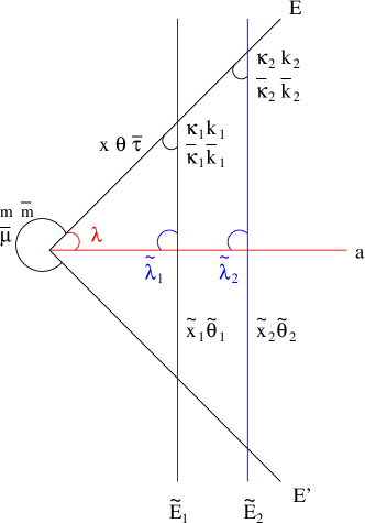
Figure 1: Multi-instanton configuration involving two O(1) instantons.

We can now analyse the combined instanton effective action involving these fields. In this section we start on the hypersurface in complex structure moduli space where the $U(1)$ instanton $E$ is supersymmetric with respect to the orientifold plane. On this locus, the bosonic modes are massless. The relevant parts of the effective action of the multi-instanton effective action first include the couplings

$$S_{1}=Y_{1ij}\left(\kappa^{\alpha}_{1}\widetilde{\theta}_{1\alpha}\,\widetilde{\lambda}^{i}_{1}\,\lambda^{j}+k_{1}\widetilde{\lambda}^{i}_{1}\,\lambda^{j}\right)\quad\quad+\quad\quad(1\leftrightarrow 2)$$ (17)

involving the charged modes $\lambda^{i}$ which we are trying to lift. For their computation see [8].

A second class of couplings can be understood as coming from F-terms of the type

$$W\simeq\sum_{i=1}^{2}M\,K_{i}\,K_{i},$$ (18)

where $K_{i}$ formally denotes the superfield associated with the zero modes $(k_{i},\kappa_{i}^{\alpha})$ and similarly for $M$ . In components the fermionic terms are

$$S_{2}={\overline{L}}_{1}\left(\overline{\mu}^{\dot{\alpha}}\,\overline{\kappa}_{1\dot{\alpha}}\,\overline{k}_{1}+\overline{m}\,\overline{\kappa}_{1}^{\dot{\alpha}}\,\overline{\kappa}_{1\dot{\alpha}}\right)+L_{1}m\,\kappa_{1}^{\alpha}\,\kappa_{1\alpha}\quad\quad+\quad\quad(1\leftrightarrow 2),$$ (19)

where we introduced the physical coupling constants $L_{1}$, $L_{2}$. These are related to the holomorphic coupling constants $l_{1}$ and $l_{2}$ via (95) described in appendix B.

A third class of interactions consists of the couplings [17]

$$S_{3}=C_{m}\,(m\,\overline{\mu}^{\dot{\alpha}}\,\overline{\tau}_{\dot{\alpha}})+C_{k_{1}}\,(\overline{\kappa}_{1}^{\dot{\alpha}}\,\overline{\tau}_{\dot{\alpha}}\,k_{1})+C_{k_{2}}\,(\overline{\kappa}_{2}^{\dot{\alpha}}\,\overline{\tau}_{\dot{\alpha}}\,k_{2}).$$ (20)

The bosonic fields furthermore enter the D-term for $U(1)_{E}$ in the usual way as

$$S_{D}=\frac{1}{2g^{2}_{E}}\,(2m\overline{m}-k_{1}\overline{k}_{1}-k_{2}\overline{k}_{2}-\xi)^{2},$$ (21)

where the gauge coupling of the instanton theory $\frac{1}{g^{2}_{E}}=\frac{1}{g_{s}}\frac{{\rm Vol}_{E2}}{\ell_{s}^{3}}$ induces an inverse scaling with $g_{s}$, as will become crucial later on. Besides, the F-term potential associated with the above trilinear couplings reads

$$S_{F}=l_{1}^{2}|m\,k_{1}|^{2}+l_{2}^{2}|m\,k_{2}|^{2}+|l_{1}k_{1}^{2}+l_{2}k_{2}^{2}|^{2}.$$ (22)

With the help of the above coupling terms we can indeed saturate all fermionic zero modes other than the universal $\theta^{\alpha}$ required for superpotential contributions of $E$. Concretely, we pull down

$$Y_{1ij}\,Y_{2kl}\ \times\,\quad(\kappa^{\alpha}_{1}\widetilde{\theta}_{1\alpha}\,\widetilde{\lambda}^{i}_{1}\,\lambda^{j})\,\,\,(\kappa^{\alpha}_{2}\widetilde{\theta}_{2\alpha}\,\widetilde{\lambda}^{k}_{2}\,\lambda^{l})$$ (23)

with $i\neq k$ and $j\neq l$ in the instanton path integral. The remaining fermionic modes can be absorbed by the product

$$C_{k_{1}}\,C_{k_{2}}\,\overline{L}_{1}\,\overline{L}_{2}\,\,(k_{1}\,\overline{\kappa}_{1}\,\overline{\tau})\,\,(\overline{\mu}\,\overline{\kappa}_{1}\,\overline{k}_{1})\,\,(k_{2}\,\overline{\kappa}_{2}\,\overline{\tau})\,\,(\overline{\mu}\,\overline{\kappa}_{2}\,\overline{k}_{2}).$$ (24)

Schematically, we are left with the nonvanishing, finite bosonic integral

$$Y^{2}_{1ij}\,Y^{2}_{2kl}\,\overline{L}_{1}\,\overline{L}_{2}\,\int dk_{1}\,d\overline{k}_{1}\,\,dk_{2}\,d\overline{k}_{2}\,\,dm\,d\overline{m}\,\,\,\,|k_{1}|^{2}\,|k_{2}|^{2}\,\,\,\,exp(-S_{D}-S_{F}).$$ (25)

Instead of (24) we can also saturate the remaining fermionic modes by

$$(C_{m})^{2}\,\overline{L}_{1}\,\overline{L}_{2}\,\,(m\,\overline{\mu}\,\overline{\tau})^{2}\,\,\overline{m}\,\overline{\kappa}_{1}\,\overline{\kappa}_{1}\,\,\overline{m}\,\overline{\kappa}_{2}\,\overline{\kappa}_{2},$$ (26)

which leads to the non-vanishing bosonic integral

$$Y^{2}_{1ij}\,Y^{2}_{2kl}\,\overline{L}_{1}\,\overline{L}_{2}\,\int dk_{1}\,d\overline{k}_{1}\,\,dk_{2}\,d\overline{k}_{2}\,\,dm\,d\overline{m}\,\,\,\,|m|^{4}\,\,\,\,exp(-S_{D}-S_{F}).$$ (27)

As a result of summing up all different channels, the multi-instanton BPS configuration produces a non-vanishing contribution to the superpotential. The scale of this contribution is set by the exponentiated classical instanton action,

$$W\simeq exp\left(-\frac{2\pi}{\ell_{s}^{3}}(\int_{\Xi}\frac{1}{g_{s}}\Omega+iC_{3}+\int_{\widetilde{\Xi}_{1}}\frac{1}{g_{s}}\Omega+iC_{3}+\int_{\widetilde{\Xi}_{2}}\frac{1}{g_{s}}\Omega+iC_{3})\right).$$ (28)

As in single instanton computations, this classical suppression factor is multiplied by the exponentiated sum over all one-loop annulus diagrams with one end on the instantons and one end on the D6-branes of the model, $\sum_{b}Z^{\prime}_{A}(E2,D6_{b})$, together with the Möbius amplitudes $M^{\prime}(E2,O6)$ [1]. Here $E2=E,\widetilde{E}_{1},\widetilde{E}_{2}$ and the massless modes are excluded. As an important consistency check, holomorphicity of the generated superpotential is ensured by the cancellation of the non-holomorphicities in the physical couplings $\overline{L}_{i}$, $Y_{1jk}$, $Y_{2jk}$ appearing in (23), (24), (26), partially among one another and partially with the non-holomorphic part of these one-loop amplitudes. More details are given in the context of our concrete example at the end of appendix B.

Before proceeding we would like to notice that the simpler configuration consisting of the $U(1)$ instanton pair and only one $O(1)$ instanton does not induce a superpotential. While for suitable intersection numbers the resulting effective action may contain the couplings required to saturate all extra fermionic zero modes, the complex integral over the bosonic modes contains now a monomial in $m^{a}k^{b}$ and not in $|m|^{a}|k|^{b}$. It vanishes as a result of the uncancelled relative phase. We will come back to this point at the end of the next section.

3.3 (Non-)BPS bound states and contributions to the superpotential

I.) $\xi>0$

Now we deform the complex structure of the Calabi-Yau manifold away from the line of marginal stability ${\cal M}_{0}$ determined by $\xi=0$ for the cycles $\Xi$ and $\Xi^{\prime}$. For simplicity we assume we can take a path in complex moduli space along which the calibration of the other D-branes remains unchanged .

Due to the strictly chiral nature of the intersection of the cycle $\Xi$ with its image $\Xi^{\prime}$, (33), it is possible only for deformations into $\cal M_{+}$ where $\xi>0$ that $\Xi$ and $\Xi^{\prime}$ combine into a new special Lagrangian cycle

$$Y=E^{\prime}\#E$$ (29)

with homological charge $[E]+[E^{\prime}]$ and which preserves the same ${\cal N}=1$ supersymmetry as the orientifold. The bound state $Y$ disappears from the spectrum of BPS branes on the other side in complex moduli space, i.e in ${\cal M}_{-}$. It is therefore an interesting question how the instanton-induced superpotential behaves as the line of marginal stability is crossed.

Let us begin with small deformations leading to formation of the BPS bound state $Y$. From the effective field theory point of view, the Fayet-Iliopoulos parameter $\xi$ for $U(1)_{E}$ becomes positive and renders the bosons $m,\overline{m}$ tachyonic. At the end of the recombination process $m,\overline{m}$ have acquired a VEV such that D-flatness is preserved. The fluctuation modes $\delta m$ and $\delta\overline{m}$ become massive via the D-term, and so do the fermions $\overline{\mu}^{\dot{\alpha}}$ and $\overline{\tau}^{\dot{\alpha}}$ through the coupling $\langle m\rangle\,\overline{\mu}\,\overline{\tau}$. The VEV for $m$ and $\overline{m}$ likewise induces a mass term for the bosonic modes $k_{i},\overline{k}_{i}$ and the fermions $\kappa_{i}^{\alpha}$ and $\overline{\kappa}_{i}^{\dot{\alpha}}$.

The only massless modes of the multi-instanton system (besides $x^{\mu},\theta^{\alpha}$ and $\widetilde{x}_{i}^{\mu}$) are the charged modes $\lambda^{i}$, $\widetilde{\lambda}^{j}$ together with $\widetilde{\theta}_{1}^{\alpha},\widetilde{\theta}_{2}^{\alpha}$. From general ${\cal N}=2$ worldsheet arguments there should exist the six-point couplings

$$\langle\widetilde{\theta}_{1}^{\alpha}\,\widetilde{\theta}_{1}^{\beta}\,\,\widetilde{\lambda}^{i}\lambda^{j}\widetilde{\lambda}^{k}\lambda^{l}\rangle+1\leftrightarrow 2.$$ (30)

The easiest way to see this is to put the vertex operators for the respective zero modes in the following pictures,

$$\langle V^{1/2}_{1/2}(\widetilde{\theta}_{1}^{\alpha})\,\,V^{-1/2}_{3/2}(\widetilde{\theta}_{1}^{\beta})\,\,\,V^{-1/2}_{-1/2}(\widetilde{\lambda}^{i})\,\,\,V^{-1/2}_{-1/2}(\lambda^{j})\,\,\,V^{-1/2}_{-1/2}(\widetilde{\lambda}^{k})\,\,\,V^{-1/2}_{-1/2}(\lambda^{l})\rangle,$$ (31)

where the superscript denotes the ghost picture and the subscript the worldsheet $U(1)$ charge. Pulling down these two couplings therefore saturates all extra fermionic modes, and the instanton bound state $(E^{\prime}\#E)\cup\,\widetilde{E}_{1}\cup\,\widetilde{E}_{2}$ contributes to the superpotential.

There is an alternative way to describe the system by thinking of the instantons wrapping the individual cycles $\Xi,\Xi^{\prime},\widetilde{\Xi}_{1}$ and $\widetilde{\Xi}_{2}$ before formation of the bound state $Y$ in the following way: As $\Xi$ and $\Xi^{\prime}$ are at non-supersymmetric angles, the open string excitations describing the bosons $m,\overline{m}$ are tachyonic, while the ones corresponding to $k_{i},\overline{k}_{i}$ acquire positive ${\rm(mass)}^{2}$. From the quantisation of the open string modes it is furthermore clear that in this picture, i.e. prior to condensation of $m,\overline{m}$, all fermionic modes remain massless. The instanton effective action for this system is obtained by integrating out the bosonic non-zero modes and keeping only the couplings involving the fermionic zero modes. In fact, non-zero instanton modes are strictly off-shell as it is not possible, in absence of four-dimensional momentum, to write down a consistent vertex operator for massive excitations. This is reflected in the usual procedure to allow for the non-zero modes to appear only in the one-loop amplitudes.

The effective coupling replacing the interactions (19) and (20) upon integrating out $k_{i}$ and $\overline{k}_{i}$ become

$$S^{\prime}=\overline{\mu}\,\overline{\kappa}_{1}\,\overline{\kappa}_{1}\,\overline{\tau}+\overline{\mu}\,\overline{\kappa}_{2}\,\overline{\kappa}_{2}\,\overline{\tau}.$$ (32)

These terms allow us to saturate all extra fermionic zero modes, reproducing the conclusion that the instanton system contributes to the superpotential.

II.) $\xi<0$

Now we deform the complex structure such as to enter the region ${\cal M}_{-}$ of moduli space where the special Lagrangian $Y$ ceases to exist. However, as encoded already in the D-term potential (34), $E$ can recombine instead with the $O(1)$ instantons on the cycles $\widetilde{\Xi}_{1}$ or $\widetilde{\Xi}_{2}$. The D-term only fixes the combination $|k_{1}|^{2}+|k_{2}|^{2}$ and leaves us with one complex bosonic modulus consisting of the orthogonal combination as well as the relative phase between the complex fields $k_{1}$ and $k_{2}$. Both are fixed by the F-term in a D- and F-flat manner. The non-zero VEV for $k_{1}$ and $k_{2}$ also renders the boson $m$ massive. All extra fermionic modes $\widetilde{\lambda}_{i}$, $\lambda_{j}$, $\kappa_{k}$ and $\overline{\kappa}_{l}$ acquire a mass via their couplings to $k_{i}$.

This shows how holomorphicity of the D-brane instanton induced superpotential is maintained even in situations where specific BPS instantons disappear across lines of marginal stability. In ${\cal M}_{+}$ the superpotential is corrected by instantons wrapping the BPS configuration $(E^{\prime}\#E)\cup\,\widetilde{E}_{1}\cup\,\widetilde{E}_{2}$. It is a multi-instanton configuration with constituents $\widetilde{E}_{1}$, $\widetilde{E}_{2}$ and the BPS bound state $Y=E^{\prime}\#E$. Along ${\cal M}_{0}$ this bound state $Y$ meets a line of marginal stability, but the multi-instanton $E\cup E^{\prime}\cup\,\widetilde{E}_{1}\cup\,\widetilde{E}_{2}$ is still BPS and contributes to the superpotential. In ${\cal M}_{-}$ the former BPS state $Y=E^{\prime}\#E$ has disappeared, but ther exists a new BPS state $\Psi=\widetilde{E}_{1}\#(E\cup E^{\prime})\#\widetilde{E}_{2}$ with charge $[E]+[E^{\prime}]+[\widetilde{E}_{1}]+[\widetilde{E}_{1}]$. The two additional instantons $\widetilde{E}_{1}$ and $\widetilde{E}_{2}$ required to lift the fermionic zero modes for $\xi=0$ conspire such that the number of BPS states of total charge $[E]+[E^{\prime}]+[\widetilde{E}_{1}]+[\widetilde{E}_{1}]$ does not jump across the line of marginal stability.

To illustrate this connection further, it is instructive to analyse how a jump in the BPS spectrum is correlated with a microscopic obstruction to a superpotential contribution already at threshold. The simplest example would of course be just the $U(1)$ instanton and its image which cannot contribute due to extra charged modes. But there are even more subtle obstructions to superpotential contributions in agreement with a discontinuous BPS spectrum.

Consider the lifting of the charged zero modes by a single $O(1)$ instanton wrapping the cycle $\widetilde{\Xi}$. In order to lift the additional 4 charged zero modes $\lambda$ we require e.g.

$$[\widetilde{\Xi}_{1}\cap\Pi_{a}]^{+}=4,\quad\quad\quad[\Xi\cap\widetilde{\Xi}_{1}]^{+}=1.$$ (33)

Such a setup is depicted in figure 2. The massless spectrum comprises $4$ additional charged zero modes $\tilde{\lambda}$ the bosonic and fermionic zero modes $k$ and $\kappa^{\alpha}$ and their conjugates and finally the universal zero modes $\tilde{x}$ and $\tilde{\theta}^{\alpha}$ of the $O(1)$ instanton.

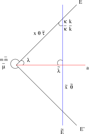
Figure 2: Multi-instanton configuration involving a single O(1) instanton.

One observes the same couplings as in (17), (19) and (20), but the D-term and the F-term now take the form

$$S_{D}=\frac{1}{2g^{2}_{E}}\,(2m\overline{m}-k\overline{k}-\xi)^{2},\qquad S_{F}=l_{1}^{2}\left((k\,\overline{k})^{2}+|m\,k|^{2}\right).$$ (34)

As before we can saturate all charged zero modes $\lambda$ and $\tilde{\lambda}$ by pulling down

$$Y_{ij}\,Y_{kl}\ \times\,\quad(\kappa^{\alpha}\widetilde{\theta}_{\alpha}\,\widetilde{\lambda}^{i}\,\lambda^{j})\,\,\,(k\,\widetilde{\lambda}^{k}\,\lambda^{l}),$$ (35)

while the remaining fermionic zero modes can be absorbed by

$$C_{k}\,C_{m}\,\overline{L}\,\,(k\,\overline{\kappa}\,\overline{\tau})\,\,(\overline{\mu}\,\overline{\kappa}\,\overline{k})\,\,(\overline{\mu}\,m\,\overline{\tau}).$$ (36)

This leaves us with the bosonic integral

$$Y^{4}_{ij}\,C_{k}\,\overline{L}\,\int dk\,d\overline{k}\,\,dm\,d\overline{m}\,\,\,\,|k|^{2}\,k^{2}\,m\,\,\,\,exp(-S_{D}-S_{F}).$$ (37)

Unlike in the previous case this vanishes after integrating over the relative phase between $m$ and $k$. Alternatively one can saturate all fermionic zero modes via the couplings

$$C^{2}_{m}\,\overline{L}\,\,(\overline{m}\,\overline{\kappa}\,\overline{\kappa})\,\,\,(\overline{\mu}\,m\,\overline{\tau})^{2}$$ (38)

leading to the bosonic integral

$$Y^{4}_{ij}\,C^{2}_{m}\,\overline{L}\,\int dk\,d\overline{k}\,\,dm\,d\overline{m}\,\,\,\,|m|^{2}\,k^{2}\,m\,\,\,\,exp(-S_{D}-S_{F}).$$ (39)

Again this integral vanishes and there are no superpotential contributions.

This is consistent with the behaviour of such an instanton configuration for a small deformation of the complex structure. The configuration is very similar to the D-brane setup discussed in section 2.2. For sufficiently small deformations of the complex structure the new stable geometric object is described by condensation of the bosonic modes such that the potential $V=S_{D}+\,S_{F}$ is minimized. For $\xi<0$, this happens at

$$|k|=\sqrt{-\frac{\xi}{1+a}},\quad\quad m=0,$$ (40)

where $a=2g^{2}_{E}\,l<<1$. Note that this minmum breaks both D-flatness and F-flatness. It corresponds to an instanton wrapping the bound state $\widetilde{\Psi}$ of the cycle $\Xi\cup\Xi^{\prime}$ with $\widetilde{\Xi}$.

This new multi-bound state $\widetilde{\Psi}$ is truly non-BPS. As in section 2.2 a possible way to think about $\widetilde{\Psi}$ is as a deformation of the sLag $\Psi$ defined as the would-be BPS bound state formed by $\widetilde{\Xi}$, $\Xi$ and $\Xi^{\prime}$ if the superpotential (18) were absent, i.e. $l=0$. From the field theory point of view, the tachyon $k$ would condense as $|k|=\sqrt{-{\xi}}$ and the excitation mode $\delta k$ around this vacuum expectation value would be massive. Now by switching on $l\neq 0$, $m$ acquires a mass. The F-terms also induce a term linear in the massive fields $\delta k$. This indicates that the system is unstable towards formation of the metastable non-BPS state $\widetilde{\Psi}$. In the spirit of the discussion at the end of section 2.2, $\widetilde{\Psi}$ is a non-calibrated Lagrangian three-cycle.

Such a non-supersymmetric state is not expected to contribute to the superpotential, thus on the line of margin stability $\xi=0$ there should not be any contributions either. This is in complete agreement with our previous analysis.

4 Superpotential contributions in Type I theory

In this section we give the mirror dual description of instanton bound states for Type I compactifications on a Calabi-Yau manifold $X$. This language is particularly useful to illustrate the general ideas of section 3 in terms of very concrete and computable algebraic objects. By translating the results of the previous section into Type I we will identify a new class of instantons correcting the superpotential. By S-duality to heterotic compactifications they map to bound states of worldsheet and NS5-brane instantons carrying vector-bundles.

The building blocks of the Type I gauge sector are formed by stacks of $M_{a}=N_{a}\times n_{a}$ $D9$-branes wrapping $X$ and carrying stable holomorphic vector bundles $V_{a}$ of rank $n_{a}$. In addition we have to add their orientifold images, given by a $D9$-brane with the dual bundle $V_{a}^{\vee}$. The associated gauge group of each stack of $D9$-branes is $U(N_{a})$. For pairs of such magnetised $D9$-branes, bifundamental matter is counted by the cohomology groups

$$H^{i}(X,V_{a}\otimes V_{b}),\quad\quad i=1,2,$$ (41)

where $i=1$ and $i=2$ respectively refer to chiral and anti-chiral superfields transforming as $(N_{a},N_{b})$. Replacing $V_{a}$ by its dual $V^{\vee}_{a}$ interchanges $N_{a}$ with the conjugate representation $\overline{N}_{a}$. More background can be found in [69, 70]. We will be working in the large volume limit where the BPS condition for the holomorphic bundles is given, in slight oversimplification, by $\mu$-stability together with

$$\mu_{J}(V)=0,\quad\quad\quad\mu_{J}(V)=\frac{1}{{\rm rk}(V)}\int_{X}J\wedge J\wedge c_{1}(V).$$ (42)

Strictly speaking, BPS bundles are not described by the category of coherent sheaves, but rather by its derived category [49]. The correct stability criterion differs from the above even in the limit $\alpha^{\prime}\rightarrow 0$, where perturbative and worldsheet instanton corrections to the definition of the $\mu$-slope can be neglected [48, 71].

The superpotential receives corrections from Euclidean $D1$-branes wrapping holomorphic curves [72]. These are dual to the described $O(1)$ instantons in Type IIA. In the sequel it will be useful to model an $E1$ instanton wrapping the curve $C$ as the sheaf ${\cal O}|_{C}$. For a detailed description of $E1$-instantons in this language we refer the reader to [23].

One of the motivations for this work was to investigate whether the superpotential also receives contributions from Euclidean $D5$-branes on $X$. Such $E5$-instantons without additional gauge flux carry gauge group $Sp(2)$ and therefore exhibit too many Goldstone modes to contribute to the superpotential at least in a straightforward manner. Instead we consider $E5$-instantons with non-vanishing worldvolume flux. Note that these are dual in Type IIA theory to $E2$-instantons of $U(1)$ type, which can meet lines of marginal or threshold stability and were considered in the previous sections.

Similarly to the IIA context, we begin with a configuration of BPS $E5$-instantons carrying stable holomorphic bundles with zero slope, together with their orientifold image. For practical reasons we will mostly focus on $E5$-branes endowed with complex line bundles $L$ (together with their image $E5$-branes with $L^{\vee}$). This can be generalised to bundles of higher rank.

We are interested in studying the transition of this system, i.e. of the direct sum of instanton bundles

$$\widetilde{V}=L\oplus L^{\vee},$$ (43)

to non-split extension bundles upon crossing a line of marginal stability in Kähler moduli space. The two possible bound states $V=L^{\vee}\#L$ and $U=L\#L^{\vee}$ can be thought of as the extensions given by

$$0\rightarrow L\rightarrow V\rightarrow L^{\vee}\rightarrow 0$$ (44)

and

$$0\rightarrow L^{\vee}\rightarrow U\rightarrow L\rightarrow 0,$$ (45)

respectively. Non-splitness and thus existence of the extensions $V$ or $U$ requires that the groups ${\rm Ext}^{1}_{X}(L^{\vee},L)=H^{1}(X,L^{2})$ or ${\rm Ext}^{1}_{X}(L,L^{\vee})=H^{1}(X,(L^{\vee})^{2})$ are non-zero, respectively. A necessary condition for stability of a non-split extension is that the slope of the bundle to the left be smaller than that of the extension bundle. In general this is not sufficient yet, but for small enough deformations away from ${\cal M}_{0}$, i.e. for sufficiently small slope, stability is expected on physical grounds (see also [60]). The recombination (or extension) modes $m,\overline{m}$ or $n,\overline{n}$ in the $L-L^{\vee}$ sector triggering formation of $V$ or $U$, respectively, are summarized in table 3.

zero mode	$Q_{E}$	Cohomology
$m$	$2$	$H^{1}(X,L^{2})$
$\overline{m}$, $\overline{\mu}^{\dot{\alpha}}$	$-2$	$H^{2}(X,(L^{\vee})^{2})$
$n$	$-2$	$H^{2}(X,L^{2})$
$\overline{n}$, $\overline{\nu}^{\dot{\alpha}}$	$2$	$H^{1}(X,(L^{\vee})^{2})$

Table 3: Extension modes in $L-L^{\vee}$ sector.

The direct sum $\widetilde{V}$ represents a BPS instanton along the real codimension 1 hypersurface ${\cal M}_{0}$ in Kähler moduli space defined by $\mu_{J}(L)=0=\mu_{J}(\widetilde{V})$. Upon deforming $J$ such that $\mu_{J}(L)<0$ we enter into ${\cal M}_{+}$ where the bound state $V$ forms, while $U$ can exists for $J\in{\cal M}_{-}$ defined by $\mu_{J}(L)>0$.

In this language it is particularly obvious that objects of a given charge vector can meet several lines of marginal/threshold stability in moduli space and that the type of these hypersurfaces can vary. In our case this corresponds to the existence of two different line bundles $L_{1}$, $L_{2}$ with

$${\rm ch}(L_{1})+{\rm ch}(L_{1}^{\vee})={\rm ch}(V)={\rm ch}(L_{2})+{\rm ch}(L_{2}^{\vee}),\quad H^{1}(X,L_{1}^{2})\neq 0\neq H^{1}(X,L_{2}^{2}).$$ (46)

Since ${\rm ch}_{i}(L^{\vee})=(-1)^{i}\,{\rm ch}_{i}(L)$ this only constrains ${\rm ch}_{2}(L_{1})={\rm ch}_{2}(L_{2})=\frac{1}{2}{\rm ch}_{2}(V)$. By contrast, both the slope of $L_{i}$ and the index $\chi(L_{i}^{2})$ depend on the odd Chern classes. It can therefore happen that $V$ meets a line of threshold stability with respect to $L_{1},L_{1}^{\vee}$ for Kähler class $J_{1}$ and a line of marginal stability with respect to $L_{2},L_{2}^{\vee}$ for a different Kähler class $J_{2}$.

4.1 Lifting of chiral excess modes in a 2-instanton process

Consider now a tadpole free supersymmetric Type I compactification of the above type on the locus $J\in{\cal M}_{0}$. As in Type IIA one can show that the charged zero modes of the BPS $E5$-instanton carrying the direct sum bundle $\widetilde{V}$ with all $D9$-branes have total $U(1)_{E}$ charge

$$\sum_{a}Q_{a}=-4\,\chi(X,L^{2}).$$ (47)

This enforces the existence of chiral excess modes for non vector-like situations, i.e. whenever $\chi(X,L^{2})\neq 0$ . As before we turn to the simplest chiral case of $h^{1}(X,L^{2})=n^{+}=1,h^{2}(X,L^{2})=n^{-}=0$. Equ. (47) can be satisfied by numerous possible configurations all of which lead to similar conclusions.

For concreteness consider the case that there exists a single $D9$-brane with line bundle $W$ (together with its orientifold image with $W^{\vee}$) such that

$$\lambda^{i}\in H^{1}(X,W\otimes L)\simeq{\mathbb{C}}^{n+2},\,\,H^{2}(X,W\otimes L)\simeq{\mathbb{C}}^{n},$$ (48)

$$\lambda^{j}\in H^{1}(X,W^{\vee}\otimes L)\simeq{\mathbb{C}}^{n+2},\,\,H^{2}(X,W^{\vee}\otimes L)\simeq{\mathbb{C}}^{n},$$

in agreement with (47). Let us focus on the minimal case with $n=0$ where have precisely two modes $\lambda^{i}$ with charges $(1_{W},1_{E})$ and two $\lambda^{j}$ in $(-1_{W},1_{E})$. In the Type IIA dual we saw from general worldsheet arguments that no perturbative couplings in the instanton effective action can lift these chiral excess modes. In the present context such couplings for the system $\widetilde{V}$ on top of the line of marginal stability are forbidden by general properties of the chiral ring structure. The present formalism allows us to follow the fate of these modes upon formation of the bound state $V$. As detailed in appendix A, they necessarily survive as vector-like modes of the new bound state. Clearly the two statements are equivalent as the excess modes are expected to be lifted perturbatively in the recombined system precisely if there exist couplings to the recombination moduli who acquire a VEV upon recombination.

On the other hand, the lifting of the chiral excess modes via two more $O(1)$ instantons is possible in a manner totally analogous to the IIA picture, so that we can be brief. We need two more such $E1$-instantons wrapping the rigid holomorphic curves $C_{1}$ and $C_{2}$ with a charged zero mode spectrum as given in table 4. The cohomology groups follow from the general discussion in [23].

zero mode	charge	number	Cohomology
$\lambda^{i}$	$(1_{W},1_{E})$	$2$	$H^{1}(X,W\otimes L)$
$\lambda^{j}$	$(-1_{W},1_{E})$	$2$	$H^{1}(X,W^{\vee}\otimes L)$
$\widetilde{\lambda}_{1}^{i}$	$-1_{W}$	$2$	$H^{0}(C_{1},W^{\vee}|_{C_{1}}(-1))$
$\widetilde{\lambda}_{2}^{j}$	$1_{W}$	$2$	$H^{0}(C_{2},W|_{C_{2}}(-1))$
$k_{i},\kappa_{i}^{\alpha}$	$-1_{E}$	$1$	$H^{0}(C_{i},L^{\vee}|_{C_{i}}(-1))$
$\overline{k}_{i},\overline{\kappa}_{i}^{\dot{\alpha}}$	$1_{E}$	$1$	$H^{1}(C_{i},L|_{C_{i}}(-1))$

Table 4: Charged zero modes.

From Bott’s theorem applied to the $\mathbb{P}^{1}$s $C_{1},C_{2}$ this spectrum requires that

$$W|_{C_{1}}={\cal O}_{C_{1}}(-2),\quad\quad W|_{C_{2}}={\cal O}_{C_{2}}(2),$$

$$L|_{C_{i}}={\cal O}_{C_{i}}(-1),\,\,i=1,2.$$ (49)

The couplings we invoke to lift all extra fermionic zero modes are as in the IIA system. E.g. it is possible to lift the excess modes $\lambda\in H^{1}(X,W\otimes L)$ through couplings of the form

$$\langle\kappa^{\alpha}\,(\theta_{E1})_{\alpha}\,\lambda\,\widetilde{\lambda}\rangle.$$ (50)

This Yukawa coupling corresponds to the map

$$H^{0}(C_{1},L^{\vee}|_{C_{1}}(-1))\otimes H^{0}(C_{1},W^{\vee}|_{C_{1}}(-1))\otimes H^{1}(C_{1},W\otimes L|_{C_{1}})\rightarrow{\mathbb{C}},$$ (51)

which is just the pairing

$$H^{0}(C_{1},{\cal O})\otimes H^{0}(C_{1},{\cal O}(1))\longrightarrow H^{0}(C_{1},{\cal O}(1)).$$ (52)

Note that in (51) only those modes $\lambda\in H^{1}(X,W\otimes L)$ contained in the group $H^{1}(C_{1},W\otimes L|_{C_{1}})$ can couple to $\kappa^{\alpha}\,(\theta_{E1})_{\alpha}$ and $\widetilde{\lambda}^{i}$, which are localised at $C_{1}$. It is therefore to be checked in concrete examples that all $\lambda^{i}$ are indeed lifted.

Similarly, the analogue of the coupling (19), $\langle\overline{k}_{i}\,\overline{\mu}_{\dot{\alpha}}\,\overline{\kappa}^{\dot{\alpha}}_{i}\rangle$, which is the CPT conjugate version of the Yukawa coupling $MK_{i}K_{i}$, see equ. (18), corresponds to the map

$$H^{0}(C_{i},L^{\vee}|_{C_{i}}(-1))\otimes H^{1}(C_{i},L^{2}|_{C_{i}})\otimes H^{0}(C_{i},L^{\vee}|_{C_{i}}(-1))\rightarrow{\mathbb{C}}.$$ (53)

Due to the localisation of the field $K_{i}$ on $C_{i}$, $K_{i}\in H^{0}(C_{i},L^{\vee}|_{C_{i}}(-1))$, only the restriction $H^{1}(C_{i},L^{2}|_{C_{i}})$ can participate in Yukawa couplings.

In situations where all required couplings are non-zero the multi-instanton configuration on top of the line of marginal stability, $J\in{\cal M}_{0}$, yields a non-vanishing superpotential contribution. The same conclusion holds for deformations away from ${\cal M}_{0}$ into ${\cal M}_{+}$ or ${\cal M}_{-}$ . E.g. we propose that for $J\in{\cal M}_{-}$ the BPS instanton formed by $\widetilde{V}$, $C_{1}$ and $C_{2}$ contributes to the superpotential. The relevant BPS state $\Psi$ is the bound state formed by the skyscraper sheaves ${\cal O}|_{C_{i}}$ and the vector bundle $L\oplus L^{\prime}$

$$0\rightarrow{\cal O}|_{C_{1}}\rightarrow V_{1}\rightarrow L\oplus L^{\prime}\rightarrow 0,$$

$$0\rightarrow{\cal O}|_{C_{2}}\rightarrow\Psi\rightarrow V_{1}\rightarrow 0.$$ (54)

4.2 Instanton moduli

In this section we take a closer look at vector-like recombination processes associated with lines of threshold stability [17, 25]. As summarized in section 3.1, superpotential contributions of the system $L\oplus L^{\vee}$ at threshold require the presence of quartic superpotential couplings between the vector-like extension modes $m$ and $n$. After recombination these couplings lift otherwise massless moduli of the bound state which are inherited from the recombination moduli of the wrong charge that acquire no VEV. A convenient way to determine whether or not these couplings are present is therefore to compute the moduli space of deformations of an instanton bound state described by the extension of two rigid vector bundles.

For simplicity we consider the special case that $L$ is a line bundle. The bundle moduli of the self-dual vector bundle $V=V^{\vee}$ are counted by $H^{1}(X,V\otimes V^{*})$. For our extension

$$0\rightarrow L\rightarrow V\rightarrow L^{\vee}\rightarrow 0$$ (55)

$H^{i}(X,V\otimes V^{*})$ is computed from the long exact sequence induced by

$$0\rightarrow L\otimes V^{\vee}\rightarrow V\otimes V^{\vee}\rightarrow L^{\vee}\otimes V^{\vee}\rightarrow 0.$$ (56)

In turn, $H^{i}(X,L\otimes V^{\vee})$ is determined by the long exact sequence induced by

$$0\rightarrow L\otimes L\rightarrow L\otimes V^{\vee}\rightarrow L\otimes L^{\vee}\rightarrow 0.$$ (57)

This sequence is given by
0 $\rightarrow H^{0}(X,L\otimes L)$ $\rightarrow H^{0}(X,L\otimes V^{\vee})$ $\rightarrow H^{0}(X,L\otimes L^{\vee})\stackrel{{\scriptstyle f}}{{\rightarrow}}$ $\rightarrow H^{1}(X,L\otimes L)$ $\rightarrow H^{1}(X,L\otimes V^{\vee})$ $\rightarrow H^{1}(X,L\otimes L^{\vee})\rightarrow$ $\rightarrow H^{2}(X,L\otimes L)$ $\rightarrow H^{2}(X,L\otimes V^{\vee})$ $\rightarrow H^{2}(X,L\otimes L^{\vee})\rightarrow$ $\rightarrow H^{3}(X,L\otimes L)$ $\rightarrow H^{3}(X,L\otimes V^{\vee})$ $\rightarrow H^{3}(X,L\otimes L^{\vee})\rightarrow$ 0.

Recall that we assume that there exists a hypersurface ${\cal M}_{0}$ in Kähler moduli space where $\mu(L)=0$ and that there exist small deformations of the Kähler form $J$ into the region ${\cal M}_{+}$ where $\mu(L)<0<\mu(L^{\vee})$. This means that $L$ is neither ample nor anti-ample. In addition we assume that the extension $V$ is non-split and $V$ is stable for $J\in{\cal M}_{+}$ at least for sufficiently small deformations of $J$ away from ${\cal M}_{0}$.

As an immediate consequence of these assumptions $H^{0}(X,L^{2})=0=H^{3}(X,L^{2})$ and likewise for $(L^{\vee})^{2}$. Furthermore $V^{\vee}\otimes L$ is stable and of negative slope (since we are working in the regime $J\in{\cal M}_{+}$) so that $H^{0}(X,L\otimes V^{\vee})=0$. Finally, the third column just contains $H^{*}(X,L\otimes L^{\vee})=H^{*}(X,{\cal O})\simeq(\mathbb{C},0,0,\mathbb{C})$. The first line therefore implies that the coboundary map $f$ is an injection and thus of maximal rank 1. It follows that

$$h^{1}(X,L\otimes V^{\vee})=h^{1}(X,L^{2})-1,\quad\quad h^{2}(X,L\otimes V^{\vee})=h^{2}(X,L^{2}),$$ (58)

$$h^{3}(X,L\otimes V^{\vee})=1.$$ (59)

The long exact sequence induced by (56) reads
0 $\rightarrow H^{0}(X,V^{\vee}\otimes L)$ $\rightarrow H^{0}(X,V\otimes V^{\vee})$ $\rightarrow H^{0}(X,V^{\vee}\otimes L^{\vee})$ $\stackrel{{\scriptstyle h}}{{\rightarrow}}$ $\rightarrow H^{1}(X,V^{\vee}\otimes L)$ $\rightarrow H^{1}(X,V\otimes V^{\vee})$ $\rightarrow H^{1}(X,V^{\vee}\otimes L^{\vee})$ $\stackrel{{\scriptstyle g}}{{\rightarrow}}$ $\rightarrow H^{2}(X,V^{\vee}\otimes L)$ $\rightarrow H^{2}(X,V\otimes V^{\vee})$ $\rightarrow H^{2}(X,V^{\vee}\otimes L^{\vee})$ $\rightarrow$ $\rightarrow H^{3}(X,V^{\vee}\otimes L)$ $\rightarrow H^{3}(X,V\otimes V^{\vee})$ $\rightarrow H^{3}(X,V^{\vee}\otimes L^{\vee})$ $\rightarrow$ 0.

Stability of $V$ implies $h^{0}(X,V\otimes V^{\vee})=1$. Serre duality and the fact that $V=V^{\vee}$ yield, together with (59), that $h^{0}(X,V^{\vee}\otimes L^{\vee})=h^{3}(X,V^{\vee}\otimes L)=1$. Matching the dimensions of the cohomology groups of the first line thus shows that the coboundary map $h$ has to be trivial. Finally the dimension of the moduli space of the extension bundle is given by

$$h^{1}(X,V\otimes V^{\vee})=(h^{1}(X,L^{2})-1)+h^{2}(X,L^{2})-{\rm rank}\,g=h^{2}(X,V\otimes V^{\vee}),$$ (60)

where the coboundary map $g$ is given by the cup product with $H^{1}(X,L^{2})$,

$$H^{1}(X,V\otimes L^{\vee})\times H^{1}(X,L^{2})\longrightarrow H^{2}(X,V\otimes L).$$ (61)

Clearly, strictly chiral recombinations with $h^{1}(X,L^{2})=1$ and $h^{2}(X,L^{2})=0$ result in bundles with no deformation moduli, while for all other cases moduli can in principle remain. The number of remaining moduli involves in particular the rank of the map $g$, which depends on the details of the line bundle in question. There are certainly situations conceivable where $g$ is not of maximal rank so that unlifted moduli remain. For the minimal vector-like case where $h^{1}(X,L^{2})=1=h^{2}(X,L^{2})$ this happens e.g. whenever the localisation inside $X$ of the various cohomology groups appearing in (61) does not allow for a non-trivial map of this type. We leave the discussion of concrete examples for future work.

5 Discussion

The superpotential of four-dimensional Type II orientifold compactifications can receive non-perturbative corrections not only from D-brane instantons invariant under the orientifold action everywhere in moduli space, but also from objects that can become $U(1)$ instantons for certain values of the closed string moduli. In this article we have extended our previous analysis [17] of the simplest possible type of $U(1)$ instantons with chiral intersection with the orientifold to multi-instanton processes involving in addition a certain type of $O(1)$ instantons. We have shown that the specific multi-instanton configuration can yield superpotential contributions on top of its line of marginal stability. On the two different sides of this hypersurface in moduli space, BPS (multi-)bound states of different topology, but of the same total charge can form. Their contribution to the superpotential guarantees its holomorphicity, as in the case of $U(1)$ instantons with non-chiral intersection analysed in [25]. The additional instantons in this multi-instanton configuration that allow for the formation of BPS bound states are precisely of the type required for lifting all extra zero modes on the line of marginal stability and leading to a non-zero bosonic integral, and vice versa. To put tables round, this demonstrates explicitly how the possible decay of a BPS instanton into a non-BPS one somewhere in moduli space is encoded in its microscopic description at marginal stability in a consistent way to prevent a contribution to the superpotential. We have started with a pure $U(1)$ instanton at a line of marginal stability. To lift extra zero modes we have to add new instantons. But just when the resulting multi-instanton is ready to contribute to the superpotential, the line of marginal stability has turned into a line of threshold stability, and holomorphicity of the superpotential is ensured.

Another conclusion of our analysis is that even the class of relevant BPS objects is larger than mostly considered. The multi-instanton setup with $U(1)$ instantons maps to Type I $D5$-brane instantons carrying holomorphic bundles and their bound states with $D1$-instantons. These are in turn S-dual to bound states of magnetised heterotic NS5-brane instantons and worldsheet instantons. Both what we called chiral and vector-like setups involving these objects have to be analysed to compute the full superpotential. We outlined how the presence of the required couplings in the instanton worldvolume action can be determined with the help of standard algebraic techniques. It will be interesting to check in concrete compactifications if these hitherto neglected instantons yield corrections to reckon with. This is an important question not only in view of the destabilising effect that instantons may have on four-dimensional string vacua.

Acknowledgements

We thank O. Aharony, R. Blumenhagen, T. Brelidze, F. Denef, R. Donagi, M. Douglas, D. Joyce, T. Pantev, M. Schulz, S. Sethi and D. Van den Bleeken for discussions and correspondence. This research was supported in part by the National Science Foundation under Grant No. PHY99-07949, the Department of Energy Grant DOE-EY-76-02-3071 and the Fay R. and Eugene L. Langberg Endowed Chair.

Appendix A Absence of perturbative lifting of chiral excess modes

In this appendix we further substantiate the absence of non-perturbative couplings that would lift the chiral excess modes $\lambda$ in the context of $U(1)$ instantons with chiral intersections with their orientifold image.

Consider the system of section 4.1 with intersection numbers $h^{1}(X,L^{2})=1,$ $h^{2}(X,L^{2})=0$. First we investigate if couplings of the type $\langle\overline{m}\lambda^{i}\lambda^{j}\rangle$ can exist on the locus $J\in{\cal M}_{0}$. For this purpose we recall that

$$\overline{m}\in H^{2}(X,(L^{\vee})^{2}),\quad\lambda^{i}\in H^{1}(X,W\otimes L),\quad\lambda^{j}\in H^{1}(X,W^{\vee}\otimes L)$$ (62)

with $i=1,2$ and $j=3,4$. The above Yukawa coupling would correspond to a map

$$H^{2}(X,(L^{\vee})^{2})\times H^{1}(X,W\otimes L)\times H^{1}(X,W^{\vee}\otimes L)\rightarrow{\mathbb{C}}.$$ (63)

While allowed by gauge invariance, such a map can obviously not exist in view of the degrees of the cohomology groups. This is the analogue of the worldsheet argument discussed in this context in [17] and reviewed in section 3.1. Rather we would need

$$H^{1}(X,(L^{\vee})^{2})\times H^{1}(X,W\otimes L)\times H^{1}(X,W^{\vee}\otimes L)\rightarrow H^{3}(X,\cal O)\equiv{\mathbb{C}},$$ (64)

but by assumption $h^{1}(X,(L^{\vee})^{2})=0$.

The absence of couplings $\langle\overline{m}\lambda^{i}\lambda^{j}\rangle$ at ${\cal M}_{0}$ is equivalent to the statement that the $\lambda$ modes survive as vector-like modes between the bound state $V$ and the brane $W$ as we enter into ${\cal M}_{+}$. The relevant cohomology groups $H^{*}(X,W\otimes V)$ follow from the short exact sequence

$$0\rightarrow W\otimes L\rightarrow W\otimes V\rightarrow W\otimes L^{\vee}\rightarrow 0$$ (65)

obtained by tensoring (44) with the bundle $W$. It induces the long exact sequence in cohomology

$$0 \rightarrow H^{0}(X,W\otimes L)\rightarrow H^{0}(X,W\otimes V)\rightarrow H^{0}(X,W\otimes L^{\vee})\rightarrow$$ (66)

$$\rightarrow H^{1}(X,W\otimes L)\rightarrow H^{1}(X,W\otimes V)\rightarrow H^{1}(X,W\otimes L^{\vee})\rightarrow$$ (67)

$$\rightarrow H^{2}(X,W\otimes L)\rightarrow H^{2}(X,W\otimes V)\rightarrow H^{2}(X,W\otimes L^{\vee})\rightarrow$$ (68)

$$\rightarrow H^{3}(X,W\otimes L)\rightarrow H^{3}(X,W\otimes V)\rightarrow H^{3}(X,W\otimes L^{\vee})\rightarrow 0.$$ (69)

Recall that for simplicity we take $L$ to be a line bundle. By assumption, $W$ is stable and of zero slope for $J\in{\cal M}_{0}$ and also for small deformations of $J$ into ${\cal M}_{+}$. Consequently, $H^{i}(X,W\otimes L)=H^{i}(X,W\otimes L^{\vee})=0$ for $i=0,3$. Thus the first and third lines of the long exact sequence are trivial and the sequence reduces to

$$0 \rightarrow H^{1}(X,W\otimes L)\equiv{\mathbb{C}}^{n+2}\rightarrow H^{1}(X,W\otimes V)\rightarrow H^{1}(X,W\otimes L^{\vee})\equiv{\mathbb{C}}^{n}\stackrel{{\scriptstyle f}}{{\rightarrow}}$$

$$\rightarrow H^{2}(X,W\otimes L)\equiv{\mathbb{C}}^{n}\rightarrow H^{2}(X,W\otimes V)\rightarrow H^{2}(X,W\otimes L^{\vee})\equiv{\mathbb{C}}^{n+2}\rightarrow 0.$$

Here we used equ. (48) and Serre duality for $W^{\vee}\otimes L$. The minimal zero mode situation corresponds to $n=0$. It follows that

$$h^{1}(X,W\otimes V) = (n+2)+n-rk(f),$$ (70)

$$h^{2}(X,W\otimes V) = (n+2)+n-rk(f),$$ (71)

where the map $f:H^{1}(X,W\otimes L^{\vee})\longrightarrow H^{2}(X,W\otimes L)$ is given by multiplication with the group $H^{1}(X,L^{2})$. It can therefore be, in principle, of any rank up to $n$, depending on the concrete bundles. In any case we see that there always exist vector-like modes counted by $H^{1}(X,W\otimes V)$, $H^{2}(X,W\otimes V)$, only some of which (namely the modes inherited from $H^{2}(X,W\otimes L)$ and $H^{2}(X,W^{\vee}\otimes L)$, which are of the wrong $U(1)_{E}$ charge compared to the needed excess modes in $H^{1}(X,W\otimes L)$ and $H^{1}(X,W^{\vee}\otimes L)$) can be lifted by the extension provided the map $f$ is non-zero. In particular this means we can never lift the excess modes counted by $H^{1}(X,W\otimes L)$ and $H^{1}(X,W^{\vee}\otimes L)$.

One might wonder if there can exist couplings involving these vector-like zero modes given by $\lambda^{i}\in H^{1}(X,W\otimes V)$ and $\lambda^{j}\in H^{1}(X,W^{\vee}\otimes V)$. E.g. if W is a vector bundle with moduli $h\in H^{1}(X,W\otimes W^{\vee})$, one could consider couplings of the type $\langle h\lambda\lambda\rangle$, corresponding to a map

$$H^{1}(X,W\otimes V)\times H^{1}(X,W\otimes W^{\vee})\times H^{1}(X,W^{\vee}\otimes V)\rightarrow H^{3}(X,\cal O)\equiv{\mathbb{C}}.$$ (72)

As $V\simeq V^{\vee}$ this map might exist. However, as discussed above, $H^{1}(X,W\otimes V)$ and $H^{1}(X,W^{\vee}\otimes V)$ inherit their elements from $H^{1}(X,W\otimes L)$ and $H^{1}(X,W^{\vee}\otimes L)$, and no map

$$H^{1}(X,W\otimes L)\times H^{1}(X,W\otimes W^{\vee})\times H^{1}(X,W^{\vee}\otimes L)\rightarrow H^{3}(X,\cal O)\equiv{\mathbb{C}}$$ (73)

can exist.

Appendix B Local multi-instanton setup on $T^{6}/{\mathbb{Z}}_{2}\times{\mathbb{Z}}^{\prime}_{2}$

In this appendix we present a local realization of the multi-instanton effect discussed in the section 3 in a Type IIA compactification. As compactification manifold we choose $T^{6}/\mathbb{Z}_{2}\times\mathbb{Z}_{2}^{\prime}$ orientifold with Hodge numbers $(h_{11},h_{12})=(3,51)$ [73, 74] which is known to exhibit rigid cycles. We adopt the notation of [74], where further details can be found. The orbifold group is generated by $\theta$ and $\theta^{\prime}$ acting as reflection in the first and last two tori, respectively.

Each sector, $\theta$, $\theta^{\prime}$ and $\theta\theta^{\prime}$ exhibits $16$ fixed points which after blowing up give rise to additional two-cycles with the topology of ${\mathbb{P}}_{1}$. Apart from the usual non-rigid bulk cycles

$$\Pi_{a}^{B}=4\,\bigotimes_{I=1}^{3}\,(n_{a}^{I}[a^{I}]+\widetilde{m}_{a}^{I}[b^{I}]),$$ (74)

defined in terms of the fundamental one-cycles $[a^{I}],[b^{I}]$ of the $I$-th $T^{2}$ and the corresponding wrapping numbers $n_{a}^{I}$ and $\widetilde{m}_{a}^{I}=m_{a}^{I}+\beta^{I}n_{a}^{I}$ where $\beta^{I}=0,1/2$ for rectangular and tilted tori, respectively, the background also contains so-called $g$-twisted cycles

$$\Pi^{g}_{ij}=[\alpha^{g}_{ij}]\times[(n^{I_{g}},\widetilde{m}^{I_{g}})].$$ (75)

Here ${i,j}\in\{1,2,3,4\}\times\{1,2,3,4\}$ labels one of the 16 blown-up fixed points of the orbifold element $g=\theta,\theta^{\prime},\theta\theta^{\prime}\in\mathbb{Z}_{2}\times\mathbb{Z}_{2}^{\prime}$. These cycles are basically twice the product of the two cycles of the corresponding ${\mathbb{P}}_{1}$ and the $I_{g}$ invariant one cycle $[(n^{I_{g}},\widetilde{m}^{I_{g}})]$, where $I_{g}=3,1,2$ for $g=\theta,\theta^{\prime},\theta\theta^{\prime}$.

Cycles which are charged under all three twisted sectors are rigid and take the form

$$\Pi^{F}=\frac{1}{4}\Pi^{B}+\frac{1}{4}\Bigl{(}\sum_{i,j\in S_{\theta}}\epsilon^{\theta}_{ij}\Pi^{\theta}_{ij}\Bigr{)}+\frac{1}{4}\Bigl{(}\sum_{j,k\in S_{\theta^{\prime}}}\epsilon^{\theta^{\prime}}_{jk}\Pi^{\theta^{\prime}}_{jk}\Bigr{)}+\frac{1}{4}\Bigl{(}\sum_{i,k\in S_{\theta\theta^{\prime}}}\epsilon^{\theta\theta^{\prime}}_{ik}\Pi^{\theta\theta^{\prime}}_{ik}\Bigr{)}.$$ (76)

Here $S_{g}$ denotes the set of fixed points that the rigid brane runs through in the $g$-twisted sector. The $\epsilon^{g}_{ij}=\pm 1$ correspond to the two different orientation the brane can wrap the ${\mathbb{P}}_{1}$ and have to satisfy various consistency conditions [74].

The orientifold action $\Omega\mathcal{R}$ on untwisted cycles takes the usual form

$$\Omega\mathcal{R}:[(n_{1},\widetilde{m}_{1})(n_{2},\widetilde{m}_{2})(n_{3},\widetilde{m}_{3})]\rightarrow[(n_{1},-\widetilde{m}_{1})(n_{2},-\widetilde{m}_{2})(n_{3},-\widetilde{m}_{3})]$$ (77)

whereas the twisted cycles transform as

$$\Omega\mathcal{R}:\,\alpha^{g}_{ij}[(n^{I_{g}},\widetilde{m}^{I_{g}})]\rightarrow-\eta_{\Omega\mathcal{R}}\,\eta_{\Omega\mathcal{R}g}\,\alpha^{g}_{\mathcal{R}(i)\mathcal{R}(j)}[(-n^{I_{g}},\widetilde{m}^{I_{g}})],$$ (78)

where the reflection $\mathcal{R}$ leaves all fixed points of an untilted two-torus invariant and acts on the fixed points in a tilted two-torus as

$$\mathcal{R}(1)=1,\qquad\mathcal{R}(2)=2,\qquad\mathcal{R}(3)=4,\qquad\mathcal{R}(4)=3.$$ (79)

The orientifold charges $\eta_{\Omega\mathcal{R}g}=\pm 1$ are subject to the constraint

$$\eta_{\Omega\mathcal{R}}\,\eta_{\Omega\mathcal{R}\theta}\,\eta_{\Omega\mathcal{R}\theta^{\prime}}\,\eta_{\Omega\mathcal{R}\theta\theta^{\prime}}=-1.$$ (80)

In our subsequent local setup we choose them to be

$$-\eta_{\Omega\mathcal{R}}=\eta_{\Omega\mathcal{R}\theta}=\eta_{\Omega\mathcal{R}\theta\theta^{\prime}}=\eta_{\Omega\mathcal{R}\theta^{\prime}}=1.$$ (81)

In addition we assume all three tori to be tilted such that the orientifold planes are given by

$$\Pi_{O6}=-[(2,\tilde{0})(2,\tilde{0})(2,\tilde{0})]-[(2,\tilde{0})(0,\tilde{1})(0,\tilde{1})]-2[(0,\tilde{1})(2,\tilde{0})(0,\tilde{1})]-[(0,\tilde{1})(0,\tilde{1})(2,\tilde{0})].$$

The $U(1)$-instanton $E$ wraps a bulk cycle of the form

$$\Pi^{B}_{\Xi}=[(-1,0)(-1,0)(-1,0)]=[(-1,-\tilde{\frac{1}{2}})(-1,-\tilde{\frac{1}{2}})(-1,-\tilde{\frac{1}{2}})]$$ (82)

and passes through the origin in all three tori. Thus its whole homology class $\Xi$ is given by

$$\Pi^{F}_{\Xi}=\frac{1}{4}\Pi^{B}_{\Xi}+\frac{1}{4}\sum_{i,j\epsilon(13)\times(13)}\varepsilon^{\theta}_{ij}\Pi^{\theta}_{\Xi}+\frac{1}{4}\sum_{j,k\epsilon(13)\times(13)}\varepsilon^{\theta^{\prime}}_{jk}\Pi^{\theta^{\prime}}_{\Xi}+\frac{1}{4}\sum_{i,k\epsilon(13)\times(13)}\varepsilon^{\theta\theta^{\prime}}_{ik}\Pi^{\theta\theta^{\prime}}_{\Xi},$$

$$\Pi^{\theta}_{\Xi}=[((-1,-\tilde{\frac{1}{2}})],\qquad\Pi^{\theta^{\prime}}_{\Xi}=[(-1,-\tilde{\frac{1}{2}})],\qquad\Pi^{\theta\theta^{\prime}}_{\Xi}=[(-1,-\tilde{\frac{1}{2}})].$$ (83)

Its orientifold image takes the form

$$\Pi^{F}_{\Xi^{\prime}}=\frac{1}{4}\Pi^{B}_{\Xi}+\frac{1}{4}\sum_{i,j\epsilon(14)\times(14)}\varepsilon^{\theta}_{ij}\Pi^{\theta}_{\Xi^{\prime}}+\frac{1}{4}\sum_{j,k\epsilon(14)\times(14)}\varepsilon^{\theta^{\prime}}_{jk}\Pi^{\theta^{\prime}}_{\Xi^{\prime}}+\frac{1}{4}\sum_{i,k\epsilon(14)\times(14)}\varepsilon^{\theta\theta^{\prime}}_{ik}\Pi^{\theta\theta^{\prime}}_{\Xi^{\prime}},$$

$$\Pi^{B}_{\Xi^{\prime}}=[(-1,\tilde{\frac{1}{2}})(-1,\tilde{\frac{1}{2}})(-1,\tilde{\frac{1}{2}})],$$ (84)

$$\Pi^{\theta}_{\Xi^{\prime}}=[((-1,\tilde{\frac{1}{2}})],\qquad\Pi^{\theta^{\prime}}_{\Xi^{\prime}}=[(-1,\tilde{\frac{1}{2}})],\qquad\Pi^{\theta\theta^{\prime}}_{\Xi^{\prime}}=[(-1,\tilde{\frac{1}{2}})].$$

With the intersection formulae

$$\Pi^{B}_{a}\circ\Pi^{B}_{b}=4\prod^{3}_{i=1}(n^{i}_{a}\widetilde{m}^{i}_{b}-n^{i}_{b}\widetilde{m}^{i}_{a}),$$

$$\Pi^{g}_{ij}\circ\Pi^{h}_{kl}=4\delta^{gh}\,\delta^{ik}\,\delta^{jl}(n^{I_{g}}_{a}\widetilde{m}^{I_{h}}_{b}-n^{I_{h}}_{b}\widetilde{m}^{I_{g}}_{a})$$ (85)

it is easy to show that

$$\Pi_{\Xi^{\prime}}\circ\Pi_{\Xi}=1,\qquad\Pi_{O6}\circ\Pi_{\Xi}=1.$$ (86)

As discussed in section 3.1 we need $4$ additional charged zero modes between $E$ and some D-brane $a$. We choose the brane $a$ wrapping the cycle

$$\Pi^{F}_{a}=\frac{1}{4}\Pi^{B}_{a}+\frac{1}{4}\sum_{i,j\epsilon(12)\times(34)}\varepsilon^{\theta}_{ij}\Pi^{\theta}_{a}+\frac{1}{4}\sum_{j,k\epsilon(12)\times(34)}\varepsilon^{\theta^{\prime}}_{jk}\Pi^{\theta^{\prime}}_{a}+\frac{1}{4}\sum_{i,k\epsilon(34)\times(34)}\varepsilon^{\theta\theta^{\prime}}_{ik}\Pi^{\theta\theta^{\prime}}_{a}$$ (87)

with

$$\Pi^{B}_{a}=[(0,1)(-4,3)(-4,3)]=[(0,\tilde{1})(-4,\tilde{1})(-4,\tilde{1})],\,\,\,$$ (88)

$$\Pi^{\theta}_{a}=[(-4,\tilde{1})],\qquad\Pi^{\theta^{\prime}}_{a}=[(0,\tilde{1})],\qquad\Pi^{\theta\theta^{\prime}}_{a}=[(-4,\tilde{1})].$$ (89)

Note that in contrast to section 3.2 we choose the D-brane to be not invariant under the orientifold action. Thus we additionally have to ensure $\Pi_{\Xi}\circ\Pi_{a}^{\prime}=0$ for its orientifold image $a^{\prime}$, which is indeed satisfied. In order to satisfy supersymmetry we choose the complex structure moduli $U^{I}$ to be

$$U^{1}=\frac{8}{3}\,\,,\qquad\qquad U^{2}=4\,\,,\qquad\qquad U^{3}=4\,\,.$$ (90)

As described in [17] the ${\overline{\tau}}_{\dot{\alpha}}$- and ${\overline{\mu}}_{\dot{\alpha}}$-modes can be soaked up by the coupling $m{\overline{\tau}}_{\dot{\alpha}}{\overline{\mu}}^{\dot{\alpha}}$ but there is no way to absorb the charged zero modes $\lambda$ unless we take into account additional $O(1)$-instantons. Indeed there are two instantons satisfying the constraints (33). Their homology classes are given by

$$\Pi^{F}_{\widetilde{\Xi}_{1}}=\frac{1}{4}\Pi^{B}_{\widetilde{\Xi}_{1}}+\frac{1}{4}\sum_{i,j\epsilon(12)\times(12)}\varepsilon^{\theta}_{ij}\Pi^{\theta}_{\widetilde{\Xi}_{1}}+\frac{1}{4}\sum_{j,k\epsilon(12)\times(12)}\varepsilon^{\theta^{\prime}}_{jk}\Pi^{\theta^{\prime}}_{\widetilde{\Xi}_{1}}+\frac{1}{4}\sum_{i,k\epsilon(12)\times(12)}\varepsilon^{\theta\theta^{\prime}}_{ik}\Pi^{\theta\theta^{\prime}}_{\widetilde{\Xi}_{1}},$$ (91)

$$\Pi^{F}_{\widetilde{\Xi}_{2}}=\frac{1}{4}\Pi^{B}_{\widetilde{\Xi}_{2}}+\frac{1}{4}\sum_{i,j\epsilon(34)\times(12)}\varepsilon^{\theta}_{ij}\Pi^{\theta}_{\widetilde{\Xi}_{2}}+\frac{1}{4}\sum_{j,k\epsilon(12)\times(12)}\varepsilon^{\theta^{\prime}}_{jk}\Pi^{\theta^{\prime}}_{\widetilde{\Xi}_{2}}+\frac{1}{4}\sum_{i,k\epsilon(34)\times(12)}\varepsilon^{\theta\theta^{\prime}}_{ik}\Pi^{\theta\theta^{\prime}}_{\widetilde{\Xi}_{2}}$$ (92)

with

$$\Pi^{B}_{\widetilde{\Xi}_{1}}=\Pi^{B}_{\widetilde{\Xi}_{2}}=[(2,-1)(2,-1)(2,-1)]=[(2,\tilde{0})(2,\tilde{0})(2,\tilde{0})],\qquad\,\,\,$$ (93)

$$\Pi^{\theta}_{\widetilde{\Xi}_{1}}=\Pi^{\theta}_{\widetilde{\Xi}_{2}}=[(2,\tilde{0})],\qquad\Pi^{\theta^{\prime}}_{\widetilde{\Xi}_{1}}=\Pi^{\theta^{\prime}}_{\widetilde{\Xi}_{2}}=[(2,\tilde{0})],\qquad\Pi^{\theta\theta^{\prime}}_{\widetilde{\Xi}_{1}}=\Pi^{\theta\theta^{\prime}}_{\widetilde{\Xi}_{2}}=[(2,\tilde{0})].$$ (94)

Note that both cycles are invariant under the orientifold action and are separated in the first torus ensuring that the additional zero modes appearing in the $\widetilde{E}_{1}-\widetilde{E}_{2}$ sector become massive. Now it is possible to soak up all the zero modes via the couplings (17), (19) and (20).

Let us briefly discuss the holomorphicity of the superpotential based on this example. The Yukawa couplings $\overline{L}_{i}$ and $Y_{i}$ in (17) and (19), respectively take the form

$$Y_{kij}=y_{kij}\,\,\prod^{3}_{I=1}\Gamma^{\frac{1}{4}}_{1+\phi^{I}_{Ea},1-\phi^{I}_{E\tilde{E}_{k}},1-\phi^{I}_{\tilde{E}_{k}a}},\quad\overline{L}_{k}=l_{k}\,\prod^{3}_{I=1}\Gamma^{\frac{1}{4}}_{-\phi^{I}_{EE^{\prime}},\phi^{I}_{E\tilde{E}_{k}},\phi^{I}_{E\tilde{E}_{k}}},$$ (95)

where $\phi^{I}_{ij}$ denotes the intersection angle between instanton $i$ and brane or instanton $j$, respectively and

$$\Gamma_{\alpha,\,\beta,\,\gamma}=\frac{\Gamma(1-\alpha)\,\Gamma(1-\beta)\,\Gamma(1-\gamma)}{\Gamma(\alpha)\Gamma(\beta)\Gamma(\gamma)}.$$ (96)

The lowercase letters denote the holomorphic part of the Yukawa couplings, which essentially are given by the world sheet contributions. Note that the dependence on $\phi_{E\tilde{E}_{k}}$ in (25) and (27) drops out due to the inverse dependence of $Y^{2}_{ikl}$ to $\overline{L}_{i}$. In addition there are also non-holomorphic contributions from the annulus diagrams $A(E,a)$ and $A(\tilde{E}_{k},a)$ as well as the Möbius diagram $M(E,O6)$ [1]. In our example they are given by [13, 76, 77]

$$\exp(A^{n.h.}(E,a)) =\left(\frac{\Gamma(1+\phi^{1}_{Ea})\Gamma(1+\phi^{2}_{Ea})\Gamma(1+\phi^{3}_{Ea})}{\Gamma(-\phi^{1}_{Ea})\Gamma(-\phi^{2}_{Ea})\Gamma(-\phi^{3}_{Ea})}\right),$$

$$\exp(A^{n.h.}(\tilde{E}_{k},a)) =\left(\frac{\Gamma(\phi^{1}_{\tilde{E}_{k}a})\Gamma(\phi^{2}_{\tilde{E}_{k}a})\Gamma(\phi^{3}_{\tilde{E}_{k}a})}{\Gamma(1-\phi^{1}_{\tilde{E}_{k}a})\Gamma(1-\phi^{2}_{\tilde{E}_{k}a})\Gamma(1-\phi^{3}_{\tilde{E}_{k}a})}\right)^{\frac{1}{2}},$$ (97)

$$\exp(M^{n.h.}(E,O6)) =\left(\frac{\Gamma(-\phi^{1}_{E^{\prime}E})\Gamma(-\phi^{2}_{E^{\prime}E})\Gamma(-\phi^{3}_{E^{\prime}E})}{\Gamma(1+\phi^{1}_{EE^{\prime}})\Gamma(1+\phi^{2}_{EE^{\prime}})\Gamma(1+\phi^{3}_{EE^{\prime}}}\right)^{\frac{1}{2}}.$$

Indeed, after plugging (95) and (97) into (25) or (27) all angle dependence cancels and one is left with a holomorphic expression for the superpotential.

Let us deform the complex structure in the first torus away from the line of marginal stability. Note that under deformation of the complex structure $U^{1}$, while keeping the complex structures in the other two tori fixed, the brane $a$ remains supersymmetric. For $U^{1}>8/3$ we induce a positive Fayet-Iliopoulus parameter $\xi$ for the $U(1)_{E}$ and as described in section 3.3 the cycles $\Xi$ and $\Xi^{\prime}$ combine into a new special Lagrangian $Y=\Xi\#\Xi^{\prime}$ preserving the same ${\cal N}=1$ supersymmetry as the orientifold. The whole multi-instanton configuration is then given by $(\Xi\#\Xi^{\prime})\cup\widetilde{\Xi}_{1}\cup\widetilde{\Xi}_{2}$. For $U^{1}<8/3$ we induce a negative $\xi$ for the $U(1)_{E}$ and the multi-instanton configuration recombines into the new BPS state $\widetilde{\Xi}_{1}\#((\Xi\cup\Xi^{\prime}))\#\widetilde{\Xi}_{2}$.

References

- [1] R. Blumenhagen, M. Cvetič, and T. Weigand, “Spacetime instanton corrections in 4D string vacua - the seesaw mechanism for D-brane models,” Nucl. Phys. B771 (2007) 113–142, hep-th/0609191.
- [2] M. Haack, D. Krefl, D. Lüst, A. Van Proeyen, and M. Zagermann, “Gaugino condensates and D-terms from D7-branes,” JHEP 01 (2007) 078, hep-th/0609211.
- [3] L. E. Ibáñez and A. M. Uranga, “Neutrino Majorana masses from string theory instanton effects,” JHEP 03 (2007) 052, hep-th/0609213.
- [4] B. Florea, S. Kachru, J. McGreevy, and N. Saulina, “Stringy instantons and quiver gauge theories,” JHEP 05 (2007) 024, hep-th/0610003.
- [5] S. A. Abel and M. D. Goodsell, “Realistic Yukawa couplings through instantons in intersecting brane worlds,” JHEP 10 (2007) 034, hep-th/0612110.
- [6] N. Akerblom, R. Blumenhagen, D. Lüst, E. Plauschinn, and M. Schmidt-Sommerfeld, “Non-perturbative SQCD Superpotentials from String Instantons,” JHEP 04 (2007) 076, hep-th/0612132.
- [7] M. Bianchi and E. Kiritsis, “Non-perturbative and Flux superpotentials for Type I strings on the Z3 orbifold,” Nucl. Phys. B782 (2007) 26–50, hep-th/0702015.
- [8] M. Cvetič, R. Richter, and T. Weigand, “Computation of D-brane instanton induced superpotential couplings - Majorana masses from string theory,” Phys. Rev. D76 (2007) 086002, hep-th/0703028.
- [9] R. Argurio, M. Bertolini, S. Franco, and S. Kachru, “Metastable vacua and D-branes at the conifold,” JHEP 06 (2007) 017, hep-th/0703236.
- [10] R. Argurio, M. Bertolini, G. Ferretti, A. Lerda, and C. Petersson, “Stringy Instantons at Orbifold Singularities,” JHEP 06 (2007) 067, arXiv:0704.0262 [hep-th].
- [11] M. Bianchi, F. Fucito, and J. F. Morales, “D-brane Instantons on the T6/Z3 orientifold,” JHEP 07 (2007) 038, arXiv:0704.0784 [hep-th].
- [12] L. E. Ibáñez, A. N. Schellekens, and A. M. Uranga, “Instanton Induced Neutrino Majorana Masses in CFT Orientifolds with MSSM-like spectra,” JHEP 06 (2007) 011, arXiv:0704.1079 [hep-th].
- [13] N. Akerblom, R. Blumenhagen, D. Lüst, and M. Schmidt-Sommerfeld, “Instantons and Holomorphic Couplings in Intersecting D- brane Models,” JHEP 08 (2007) 044, arXiv:0705.2366 [hep-th].
- [14] S. Antusch, L. E. Ibáñez, and T. Macri, “Neutrino Masses and Mixings from String Theory Instantons,” JHEP 09 (2007) 087, arXiv:0706.2132 [hep-ph].
- [15] R. Blumenhagen, M. Cvetič, D. Lüst, R. Richter, and T. Weigand, “Non-perturbative Yukawa Couplings from String Instantons,” Phys. Rev. Lett. 100 (2008) 061602, arXiv:0707.1871 [hep-th].
- [16] O. Aharony and S. Kachru, “Stringy Instantons and Cascading Quivers,” JHEP 09 (2007) 060, arXiv:0707.3126 [hep-th].
- [17] R. Blumenhagen, M. Cvetič, R. Richter, and T. Weigand, “Lifting D-Instanton Zero Modes by Recombination and Background Fluxes,” JHEP 10 (2007) 098, arXiv:0708.0403 [hep-th].
- [18] O. Aharony, S. Kachru, and E. Silverstein, “Simple Stringy Dynamical SUSY Breaking,” Phys. Rev. D76 (2007) 126009, arXiv:0708.0493 [hep-th].
- [19] M. Billó et al., “Instantons in N=2 magnetized D-brane worlds,” JHEP 10 (2007) 091, arXiv:0708.3806 [hep-th].
- [20] M. Billó et al., “Instanton effects in N=1 brane models and the Kahler metric of twisted matter,” JHEP 12 (2007) 051, arXiv:0709.0245 [hep-th].
- [21] M. Aganagic, C. Beem, and S. Kachru, “Geometric Transitions and Dynamical SUSY Breaking,” Nucl. Phys. B796 (2008) 1–24, arXiv:0709.4277 [hep-th].
- [22] P. G. Camara, E. Dudas, T. Maillard, and G. Pradisi, “String instantons, fluxes and moduli stabilization,” Nucl. Phys. B795 (2008) 453–489, arXiv:0710.3080 [hep-th].
- [23] M. Cvetič and T. Weigand, “Hierarchies from D-brane instantons in globally defined Calabi-Yau Orientifolds,” arXiv:0711.0209 [hep-th].
- [24] L. E. Ibáñez and A. M. Uranga, “Instanton Induced Open String Superpotentials and Branes at Singularities,” JHEP 02 (2008) 103, arXiv:0711.1316 [hep-th].
- [25] I. Garcia-Etxebarria and A. M. Uranga, “Non-perturbative superpotentials across lines of marginal stability,” JHEP 01 (2008) 033, arXiv:0711.1430 [hep-th].
- [26] C. Petersson, “Superpotentials From Stringy Instantons Without Orientifolds,” arXiv:0711.1837 [hep-th].
- [27] R. Blumenhagen, S. Moster, and E. Plauschinn, “Moduli Stabilisation versus Chirality for MSSM like Type IIB Orientifolds,” JHEP 01 (2008) 058, arXiv:0711.3389 [hep-th].
- [28] M. Bianchi and J. F. Morales, “Unoriented D-brane Instantons vs Heterotic worldsheet Instantons,” JHEP 02 (2008) 073, arXiv:0712.1895 [hep-th].
- [29] Y. Matsuo, J. Park, C. Ryou, and M. Yamamoto, “D-instanton derivation of multi-fermion F-terms in supersymmetric QCD,” arXiv:0803.0798 [hep-th].
- [30] R. Blumenhagen and M. Schmidt-Sommerfeld, “Power Towers of String Instantons for N=1 Vacua,” arXiv:0803.1562 [hep-th].
- [31] R. Argurio, G. Ferretti, and C. Petersson, “Instantons and Toric Quiver Gauge Theories,” arXiv:0803.2041 [hep-th].
- [32] M. Billó et al., “Classical gauge instantons from open strings,” JHEP 02 (2003) 045, hep-th/0211250.
- [33] M. Billo, M. Frau, F. Fucito, and A. Lerda, “Instanton calculus in R-R background and the topological string,” JHEP 11 (2006) 012, hep-th/0606013.
- [34] K. Becker, M. Becker, and A. Strominger, “Five-branes, membranes and nonperturbative string theory,” Nucl. Phys. B456 (1995) 130–152, hep-th/9507158.
- [35] E. Witten, “Small Instantons in String Theory,” Nucl. Phys. B460 (1996) 541–559, hep-th/9511030.
- [36] M. R. Douglas, “Branes within branes,” hep-th/9512077.
- [37] M. B. Green and M. Gutperle, “Effects of D-instantons,” Nucl. Phys. B498 (1997) 195–227, hep-th/9701093.
- [38] H. Ooguri and C. Vafa, “Summing up D-instantons,” Phys. Rev. Lett. 77 (1996) 3296–3298, hep-th/9608079.
- [39] C. Bachas, C. Fabre, E. Kiritsis, N. A. Obers, and P. Vanhove, “Heterotic/type-I duality and D-brane instantons,” Nucl. Phys. B509 (1998) 33–52, hep-th/9707126.
- [40] E. Kiritsis and N. A. Obers, “Heterotic/type-I duality in D ¡ 10 dimensions, threshold corrections and D-instantons,” JHEP 10 (1997) 004, hep-th/9709058.
- [41] C. Bachas, “Heterotic versus type I,” Nucl. Phys. Proc. Suppl. 68 (1998) 348–354, hep-th/9710102.
- [42] E. Witten, “Non-Perturbative Superpotentials In String Theory,” Nucl. Phys. B474 (1996) 343–360, hep-th/9604030.
- [43] S. S. Sethi, “Duality in string theory and quantum field theory,”. UMI-96-31586.
- [44] S. Sethi and M. Stern, “D-brane bound states redux,” Commun. Math. Phys. 194 (1998) 675–705, hep-th/9705046.
- [45] N. Dorey, T. J. Hollowood, and V. V. Khoze, “Notes on soliton bound-state problems in gauge theory and string theory,” hep-th/0105090.
- [46] N. Dorey, T. J. Hollowood, V. V. Khoze, and M. P. Mattis, “The calculus of many instantons,” Phys. Rept. 371 (2002) 231–459, hep-th/0206063.
- [47] N. Halmagyi, I. V. Melnikov, and S. Sethi, “Instantons, Hypermultiplets and the Heterotic String,” JHEP 07 (2007) 086, arXiv:0704.3308 [hep-th].
- [48] P. S. Aspinwall, “D-branes on Calabi-Yau manifolds,” hep-th/0403166.
- [49] M. R. Douglas, “D-branes, categories and N = 1 supersymmetry,” J. Math. Phys. 42 (2001) 2818–2843, hep-th/0011017.
- [50] A. Kapustin and Y. Li, “Stability conditions for topological D-branes: A worldsheet approach,” hep-th/0311101.
- [51] A. Font, L. E. Ibáñez, and F. Marchesano, “Coisotropic D8-branes and model-building,” JHEP 09 (2006) 080, hep-th/0607219.
- [52] M. Mariño, R. Minasian, G. W. Moore, and A. Strominger, “Nonlinear instantons from supersymmetric p-branes,” JHEP 01 (2000) 005, hep-th/9911206.
- [53] M. R. Douglas, B. Fiol, and C. Romelsberger, “Stability and BPS branes,” JHEP 09 (2005) 006, hep-th/0002037.
- [54] T. Bridgeland, “Stability conditions on a non-compact Calabi-Yau threefold,” Commun. Math. Phys. 266 (2006) 715–733, math/0509048.
- [55] S. Kachru and J. McGreevy, “Supersymmetric three-cycles and (super)symmetry breaking,” Phys. Rev. D61 (2000) 026001, hep-th/9908135.
- [56] F. Denef, “(Dis)assembling special Lagrangians,” hep-th/0107152.
- [57] J. de Boer, F. Denef, S. El-Showk, I. Messamah, and D. Van den Bleeken, “Black hole bound states in AdS3 x S2,” arXiv:0802.2257 [hep-th].
- [58] D. Joyce, “On counting special Lagrangian homology 3-spheres,” Contemp. Math. 314 (2002) 125–151, hep-th/9907013.
- [59] E. R. Sharpe, “Kaehler cone substructure,” Adv. Theor. Math. Phys. 2 (1999) 1441–1462, hep-th/9810064.
- [60] R. P. Thomas, “Moment maps, monodromy and mirror manifolds,” math/0104196.
- [61] T. Maillard, “Toward metastable string vacua from magnetized branes,” arXiv:0708.0823 [hep-th].
- [62] J. Kumar, “Dynamical SUSY Breaking in Intersecting Brane Models,” Phys. Rev. D77 (2008) 046010, arXiv:0708.4116 [hep-th].
- [63] L. Martucci, “D-branes on general N = 1 backgrounds: Superpotentials and D-terms,” JHEP 06 (2006) 033, hep-th/0602129.
- [64] R. Blumenhagen, M. Cvetič, P. Langacker, and G. Shiu, “Toward realistic intersecting D-brane models,” Ann. Rev. Nucl. Part. Sci. 55 (2005) 71–139, hep-th/0502005.
- [65] R. Blumenhagen, B. Körs, D. Lüst, and S. Stieberger, “Four-dimensional String Compactifications with D-Branes, Orientifolds and Fluxes,” Phys. Rept. 445 (2007) 1–193, hep-th/0610327.
- [66] O. J. Ganor, “A note on zeroes of superpotentials in F-theory,” Nucl. Phys. B499 (1997) 55–66, hep-th/9612077.
- [67] J. Distler and B. R. Greene, “Some Exact Results on the Superpotential from Calabi-Yau Compactifications,” Nucl. Phys. B309 (1988) 295.
- [68] T. W. Grimm, “Non-Perturbative Corrections and Modularity in N=1 Type IIB Compactifications,” JHEP 10 (2007) 004, 0705.3253.
- [69] R. Blumenhagen, G. Honecker, and T. Weigand, “Supersymmetric (non-)abelian bundles in the type I and SO(32) heterotic string,” JHEP 08 (2005) 009, hep-th/0507041.
- [70] R. Blumenhagen, G. Honecker, and T. Weigand, “Non-abelian brane worlds: The open string story,” hep-th/0510050.
- [71] E. Diaconescu and G. W. Moore, “Crossing the Wall: Branes vs. Bundles,” arXiv:0706.3193 [hep-th].
- [72] E. Witten, “World-sheet corrections via D-instantons,” JHEP 02 (2000) 030, hep-th/9907041.
- [73] E. Dudas and C. Timirgaziu, “Internal magnetic fields and supersymmetry in orientifolds,” Nucl. Phys. B716 (2005) 65–87, hep-th/0502085.
- [74] R. Blumenhagen, M. Cvetič, F. Marchesano, and G. Shiu, “Chiral D-brane models with frozen open string moduli,” JHEP 03 (2005) 050, hep-th/0502095.
- [75] R. Blumenhagen and E. Plauschinn, “Intersecting D-branes on shift Z(2) x Z(2) orientifolds,” JHEP 08 (2006) 031, hep-th/0604033.
- [76] N. Akerblom, R. Blumenhagen, D. Lüst, and M. Schmidt-Sommerfeld, “Thresholds for intersecting D-branes revisited,” Phys. Lett. B652 (2007) 53–59, arXiv:0705.2150 [hep-th].
- [77] R. Blumenhagen and M. Schmidt-Sommerfeld, “Gauge Thresholds and Kaehler Metrics for Rigid Intersecting D-brane Models,” JHEP 12 (2007) 072, arXiv:0711.0866 [hep-th].
- [78] M. R. Douglas, R. Reinbacher, and S.-T. Yau, “Branes, bundles and attractors: Bogomolov and beyond,” math/0604597.