BCS-BEC Crossover of a Quasi-two-dimensional Fermi Gas: the Significance of Dressed Molecules

Abstract

We study the crossover of a quasi-two-dimensional Fermi gas trapped in the radial plane from the Bardeen-Cooper-Schrieffer (BCS) regime to the Bose-Einstein condensation (BEC) regime by crossing a wide Feshbach resonance. We consider two effective two-dimensional Hamiltonians within the mean-field level, and calculate the zero temperature cloud size and number density distribution. For model 1 Hamiltonian with renormalized atom-atom interaction, we observe a constant cloud size for arbitrary detunings. For model 2 Hamiltonian with renormalized interactions between atoms and dressed molecules, the cloud size deceases from BCS to BEC side, which is consistent with the picture of BCS-BEC crossover. This qualitative discrepancy between the two models indicates that the inclusion of dressed molecules is essential for a mean-field description of quasi-two-dimensional Fermi systems, especially on the BEC side of the Feshbach resonance.

I introduction

The interest on low-dimensional Fermi systems has been recently reinvoked by the experimental developments of cooling and trapping atoms in optical lattices 1 ; 2 ; 3 and on atom chips 4 . With the aid of tuning an external magnetic field through a Feshbach resonance, these techniques provide a fascinating possibility of creating quasi-low-dimensional Fermi systems with a controllable fermion-fermion interaction. In particular, the interaction between fermions can be tuned from a Bardeen-Cooper-Schrieffer (BCS) limit to a Bose-Einstein condensation (BEC) limit, such that the BCS-BEC crossover can be studied in quasi low dimensions. The BCS-BEC crossover has been extensively studied in three-dimensional (3D) Fermi systems, where a single-channel model 5 and a two-channel model 6 are both applied to give a consistent description around a wide Feshbach resonance. This agreement between single- and two-channel models is rooted from the fact that the closed-channel (Feshbach molecule) population is negligible near a wide resonance, so it will not cause any significant difference by taking the molecules into account (as in the two-channel model) or completely neglecting them (as in the single-channel model). The BCS-BEC crossover of a uniform two-dimensional (2D) Fermi system has also been considered in connection with high-$T_{c}$ superconductors 7 , where an effective 2D Hamiltonian with renormalized fermion-fermion interaction is employed.

In this paper, we study the BCS-BEC crossover in a quasi-2D Fermi gas, first using an effective 2D Hamiltonian with renormalized atom-atom interaction (model 1) petrov-00 ; model-1 , and then a more general model with renormalized interaction between atoms and dressed molecules (model 2) kestner-07 . The dressed molecules mainly come from population of atoms in the excited levels along the strongly confined axial direction near a Feshbach resonance kestner-07 ; duan-05 . When considering the effect of a weak harmonic trap in the two loosely confined dimensions under the local density approximation (LDA), we adapt the mean-field (MF) treatment to calculate the zero temperature cloud size and number density distribution in the radial plane. We find a significant difference between the two models. By using model 2, we show that the cloud size decreases from the limiting value of a weakly interacting Fermi gas as one moves from the BCS to the BEC side of the Feshbach resonance, and approaches to the limiting value of a weakly interacting Bose gas in the BEC limit. This behavior is a signature of the BCS-BEC crossover in quasi two dimensions. On the contrary, model 1 fails to describe this crossover behavior, but predicts a constant cloud size and identical density profile for all magnetic field detunings. This discrepancy implies that the MF results given by model 1 is unreliable, even at a qualitative level. Given this qualitative discrepancy and the problem associated with model 1 for description of the two-body ground state of the system kestner-06 , it is likely that the oversimplification is rooted in the model itself instead of the mean-field approximation.

The quasi-2D geometry can be realized by arranging a one-dimensional (1D) optical lattice along the axial ($z$) direction and a weak harmonic trapping potential in the radial ($x$-$y$) plane, such that fermions are strongly confined along the $z$ direction and form a series of quasi-2D pancake-shaped clouds 3 . Each such pancake-shaped cloud can be considered as a quasi-2D Fermi gas when the axial confinement is strong enough to turn off inter-cloud tunneling. The strong anisotropy of trapping potentials introduces two different orders of energy scales, with one characterized by $\hbar\omega_{z}$ and the other by $\hbar\omega_{\perp}$, where $\omega_{z}$ ($\omega_{\perp}$) are the trapping frequencies in the axial (radial) directions. The separation of these two energy scales ($\omega_{z}\gg\omega_{\perp}$) allows us to first deal with the axial degrees of freedom and derive an effective 2D Hamiltonian, and leave the radial degrees of freedom for later treatment.

II Model 1 with renormalized atom-atom interaction

The effective 2D Hamiltonian for model 1 is obtained by assuming that the renormailied atom-atom interaction can be characterized with an effective 2D scattering length, with the latter derived from the exact two-body scattering physics petrov-00 ; model-1 . Thus, for a wide Feshbach resonance where the Feshbach-molecule population is negligible, we can write down an effective Hamiltonian only in terms of 2D fermionic operators $a_{\mathbf{k},\sigma}$ and $a_{\mathbf{k},\sigma}^{\dagger}$, with (pseudo) spin $\sigma$ and transverse momentum $\mathbf{k}=\left(k_{x},k_{y}\right)$. The model 1 Hamiltonian thus takes the form petrov-00 ; model-1 ; 7

$$H_{1} = \sum_{\mathbf{k},\sigma}\left(\epsilon_{\mathbf{k}}-\mu\right)a_{\mathbf{k},\sigma}^{\dagger}a_{\mathbf{k},\sigma}$$ (1)

$$+ \frac{V_{1}^{\text{eff}}}{L^{2}}\sum_{\mathbf{k},\mathbf{k^{\prime}},\mathbf{q}}a_{\mathbf{k},\uparrow}^{\dagger}a_{-\mathbf{k}+\mathbf{q},\downarrow}^{\dagger}a_{\mathbf{k^{\prime}},\downarrow}a_{-\mathbf{k^{\prime}}+\mathbf{q},\uparrow},$$

where $\epsilon_{\mathbf{k}}=\hbar^{2}k^{2}/(2m)$ is the 2D dispersion relation of fermions with mass $m$, $\mu$ is the chemical potential, and $L^{2}$ is the quantization area. The bare parameter $V_{1}^{\text{eff}}$ is connected with the physical one $V_{1p}^{\text{eff}}$ through the 2D renormalization relation $\left[V_{1}^{\text{eff}}\right]^{-1}=\left[V_{1p}^{\text{eff}}\right]^{-1}-L^{-2}\sum_{\mathbf{k}}\left(2\epsilon_{\mathbf{k}}+\hbar\omega_{z}\right)^{-1}$ ($\hbar\omega_{z}$ is from the zero-point energy), and $V_{1p}^{\text{eff}}=V_{1p}^{\text{eff}}(a_{s},a_{z})$ depends on the 3D scattering length $a_{s}$ and the characteristic length scale for axial motion $a_{z}\equiv\sqrt{\hbar/(m\omega_{z})}$ with the expression given in Ref. petrov-00 ; model-1 ; kestner-07 . Notice that the chemical potential $\mu$ can be a function of the radial coordinate $\mathbf{r}=(x,y)$ under LDA. In the following discussion, we choose $\hbar\omega_{z}$ as the energy unit so that $\mu$, $V_{1}^{\text{eff}}$, and $\epsilon_{\mathbf{k}}=a_{z}^{2}k^{2}/2$ become dimensionless.

By introducing a BCS order parameter (also dimensionless in unit of $\hbar\omega_{z}$) $\Delta\equiv(V_{1}^{\text{eff}}/L^{2})\sum_{\mathbf{k}}\left\langle a_{\mathbf{k},\downarrow}a_{-\mathbf{k},\uparrow}\right\rangle$, we get the zero temperature thermodynamic potential density

$$\Omega=-\frac{\Delta^{2}}{V_{1}^{\text{eff}}}+\frac{1}{L^{2}}\sum_{\mathbf{k}}\left(\epsilon_{\mathbf{k}}-\mu-E_{\mathbf{k}}\right),$$ (2)

where $E_{\mathbf{k}}=\sqrt{(\epsilon_{\mathbf{k}}-\mu)^{2}+\Delta^{2}}$ is the quasi-particle excitation spectrum. The ultraviolet divergence of the summation over $\mathbf{k}$ cancels with the renormalization term in $\left[V_{1}^{\text{eff}}\right]^{-1}$. The gap and number equations can be obtained respectively from $\partial\Omega/\partial\Delta^{2}=0$ and $n=-\partial\Omega/\partial\mu$ ($n=N/L^{2}$ is the density of particles), leading to

$$\frac{1}{V_{1p}^{\text{eff}}(a_{s},a_{z})} = \frac{\ln\left(-\mu+\sqrt{\mu^{2}+\Delta^{2}}\right)}{4\pi a_{z}^{2}},$$ (3)

$$n = \frac{\mu+\sqrt{\mu^{2}+\Delta^{2}}}{2\pi a_{z}^{2}}.$$ (4)

Notice that Eq. (3) can be rewritten as $F(a_{s},a_{z})=-\mu+\sqrt{\mu^{2}+\Delta^{2}}$, where the function $F$ absorbs all the dependence on $a_{s}$ and $a_{z}$. Thus, by substituting this expression into Eq. (4), we get a closed form for the number equation,

$$n=\frac{1}{\pi a_{z}^{2}}\left[\frac{F(a_{s},a_{z})}{2}+\mu\right].$$ (5)

Now we take into account the harmonic trapping potential $U(\mathbf{r})=(\omega_{\perp}/\omega_{z})^{2}r^{2}/(2a_{z}^{2})$ in the radial plane by writing down the position dependent chemical potential $\mu(\mathbf{r})=\mu_{0}-U(\mathbf{r})$, where $\mu_{0}$ is the chemical potential at the trap center. It can be easily shown that the spacial density profile is now a parabola, $n(\mathbf{r})=(\omega_{\perp}/\omega_{z})^{2}(R_{\mathrm{TF}}^{2}-r^{2})/(2\pi a_{z}^{4})$, with the Thomas-Fermi cloud size $R_{\mathrm{TF}}=\sqrt{2\mu_{0}}a_{z}(\omega_{z}/\omega_{\perp})$. By assigning the condition that the total number of particles in the trap is fixed by $N=\int n(\mathbf{r})d^{2}\mathbf{r}$, the cloud size takes the constant value $R_{\mathrm{TF}}=R_{\mathrm{BCS}}\equiv\sqrt{2\omega_{z}/\omega_{\perp}}(N)^{1/4}a_{z}$, which is independent on the 3D scattering length $a_{s}$. In fact, as one varies the scattering length $a_{s}$, the chemical potential at the trap center $\mu_{0}$ is adjusted accordingly such that the identical density profile is maintained.

This result of a constant cloud size is obviously inconsistent with the picture of a BCS-BEC crossover in quasi two dimensions. In fact, in a typical experiment with $a_{z}$ ($\sim\mu$m) much greater than the interatomic interaction potential $R_{e}$ ($\sim$nm), the scattering of atoms in this quasi-2D geometry is still 3D in nature. In particular, fermions will form tightly bound pairs on the BEC side of the Feshbach resonance as they do in 3D. Thus, in the BEC limit when fermion pair size $a_{\rm pair}\ll a_{z}$ and binding energy $|E_{b}|\gg\hbar\omega_{z}$, the system essentially behaves like a weakly interacting gas of point-like bosons, for which one would expect a vanishing small cloud size in the loosely confined radial plane petrov-00 ; posazhennikova-06 .

The MF result of a finite cloud size in the BEC limit from model 1 indicates a finite interaction strength between paired fermions, no matter how small they are in size. This statement can be extracted directly from the number equation (5), which can be written in the form $\mu=n\pi a_{z}^{2}-F(a_{s},a_{z})/2$. In the BEC limit, the second term on the right-hand side denotes one half of the binding energy, while the first term indicates a finite interaction energy per fermion pair since it is proportional to the number density. As a comparison, the actual equation of state for fermion pairs one should expect must take the form as for a quasi-2D Bose gas in the weakly interacting limit petrov-00

$$\mu_{B}\approx 3na_{z}a_{s},$$ (6)

in which case the quasi-2D gas is treated as a 3D condensate with the ground state harmonic oscillator wave function in the $z$-direction.

The interaction strength between paired fermions can also be derived by writing down a Bose representation for this system, where the fermionic degrees of freedom are integrated out in the BEC limit tokatly-04 . This Bose representation leads to a two-dimensional effective Hamiltonian for bosonic field $\phi({\bf r})$,

$$H_{\rm eff}=\int d{\bf r}\left[\phi^{\dagger}({\bf r})\left(-\frac{\hbar^{2}\nabla^{2}}{4m}+2U({\bf r})\right)\phi({\bf r})-\frac{g_{2}}{2}|\phi({\bf r})|^{4}\right],$$ (7)

where the quartic term characterizes the bosonic interaction. Within the stationary phase approximation, the interaction strength $g_{2}$ is calculated by the leading diagram of a four-fermion process with four external boson lines and four internal fermion propagators, leading to tokatly-04

$$g_{2}=2\sum_{{\bf p},\omega}\Lambda_{0}^{4}({\bf p})G_{0}^{2}({\bf p},\omega)G_{0}^{2}(-{\bf p},-\omega).$$ (8)

Here, $\Lambda_{0}=(-p^{2}/m+|E_{b}|)\chi_{0}({\bf p})$ is the boson-fermion vertex, $\chi_{0}({\bf p})$ is the Fourier transform of the relative wave function $\chi_{0}({\bf r})$ of two colliding fermions in the $s$-wave channel, and $G_{0}({\bf p},\omega)=(i\omega-p^{2}/2m-|E_{b}|/2)^{-1}$ is the free propagator for fermions. After summing over momentum ${\bf p}$ and Matsubara frequency $\omega$, we can directly show that $g_{2}$ indeed takes a constant value, being independent of the binding energy $|E_{b}|$ of paired fermions and hence the 3D scattering parameter $a_{s}$. Thus, we conclude that the MF theory based on model 1 fails to recover the picture of a weakly interacting Bose gas of paired fermions in the BEC limit, and can not be directly applied to describe the BCS-BEC crossover in quasi two dimensions.

III Model 2 with inclusion of dressed molecules

Having shown the problem associated with model 1, next we consider model 2 by taking into account the axially excited states via inclusion of dressed molecules. As derived in Ref. kestner-07 , the effective 2D Hamiltonian takes the form (also in unit of $\hbar\omega_{z}$),

$$H_{2} = \sum_{\mathbf{k},\sigma}\left(\epsilon_{\mathbf{k}}-\mu\right)a_{\mathbf{k},\sigma}^{\dagger}a_{\mathbf{k},\sigma}+\sum_{\mathbf{q}}\left(\frac{\epsilon_{\mathbf{q}}}{2}+\lambda_{b}-2\mu\right)d_{\mathbf{q}}^{\dagger}d_{\mathbf{q}}$$ (9)

$$+ \frac{\alpha_{b}}{L}\sum_{\mathbf{k},\mathbf{q}}\left(a_{\mathbf{k},\uparrow}^{\dagger}a_{-\mathbf{k}+\mathbf{q},\downarrow}^{\dagger}d_{\mathbf{q}}+h.c.\right)$$

$$+ \frac{V_{b}}{L^{2}}\sum_{\mathbf{k},\mathbf{k^{\prime}},\mathbf{q}}a_{\mathbf{k},\uparrow}^{\dagger}a_{-\mathbf{k}+\mathbf{q},\downarrow}^{\dagger}a_{-\mathbf{k^{\prime}},\downarrow}a_{\mathbf{k^{\prime}}+\mathbf{q},\uparrow},$$

where $d_{\mathbf{q}}^{\dagger}$ ($d_{\mathbf{q}}$) denotes the creation (annihilation) operator for dressed molecules with radial momentum $\mathbf{q}$, and $\lambda_{b}$, $\alpha_{b}$, and $V_{b}$ are the 2D effective bare detuning, atom-molecule coupling rate, and background interaction, respectively. These parameters can be related to the corresponding 3D parameters by matching the two-body physics kestner-07 . By introducing the order parameter $\Delta\equiv\alpha_{b}\left\langle d_{0}\right\rangle/L+(V_{b}/L^{2})\sum_{\mathbf{k}}\left\langle a_{\mathbf{k},\downarrow}a_{-\mathbf{k},\uparrow}\right\rangle$, we obtain the mean-field gap and number equations,

$$\frac{1}{V_{2p}^{\text{eff}}(2\mu)}=\frac{\ln\left(-\mu+\sqrt{\mu^{2}+\Delta^{2}}\right)}{4\pi a_{z}^{2}},$$ (10)

$$n=\frac{\mu+\sqrt{\mu^{2}+\Delta^{2}}}{2\pi a_{z}^{2}}+2\Delta^{2}\frac{\partial[V_{2,\mathrm{p}}^{\text{eff}}(x)]^{-1}}{\partial x}\Bigg{|}_{x=2\mu},$$ (11)

where the inverse of effective interaction is connected with the 3D physical parameters through kestner-07

$$\left[V_{2p}^{\text{eff}}(x)\right]^{-1} = \left[V_{b}+\frac{\alpha_{b}^{2}}{x-\lambda_{b}}\right]^{-1}+\frac{1}{L^{2}}\sum_{\mathbf{k}}\frac{1}{2\epsilon_{\mathbf{k}}+\hbar\omega_{z}}$$ (12)

$$=\frac{\sqrt{2\pi}}{a_{z}^{2}}\left[\left(U_{p}+\frac{g_{p}^{2}}{x-\gamma_{p}}\right)^{-1}-S_{p}(x)+\sigma_{p}(x)\right].$$

Here, $U_{p}=4\pi a_{bg}/a_{z}$, $g_{p}^{2}=\mu_{co}WU_{p}/(\hbar\omega_{z})$, and $\gamma_{p}=\mu_{co}(B-B_{0})/(\hbar\omega_{z})$ are 3D dimensionless physical parameters, where $a_{bg}$ is the background scattering length, $\mu_{co}$ is the difference in magnetic moments between the two channels, $W$ is the resonance width, and $B_{0}$ is the resonance point. The functions in Eq. (12) take the form

$$S_{p}(x) = \frac{-1}{4\sqrt{2}\pi}\int_{0}^{\infty}ds\left[\frac{\Gamma(s-x/2)}{\Gamma(s+1/2-x/2)}-\frac{1}{\sqrt{s}}\right],$$ (13)

$$\sigma_{p}(x) = \frac{\ln\left|x\right|}{4\pi\sqrt{2\pi}},$$ (14)

where $\Gamma(x)$ is the gamma function.

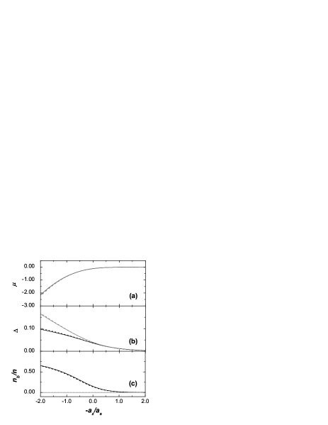
Figure 1: The BCS-BEC crossover behavior of a uniform quasi-2D Fermi gas at zero temperature, showing (a) the chemical potential $\mu$, (b) the gap $\Delta$, both in unit of $\hbar\omega_{z}$, and (c) the dressed-molecule fraction $n_{b}/n$. Notice that the results for ⁶Li (solid) and those for ⁴⁰K (dashed) almost coincide as plotted as functions of $a_{z}/a_{s}$, indicating a universal behavior around the resonance point. Furthermore, significant difference between model 1 (gray) and model 2 (black) can be observed in (b) and (c), which shows that model 1 is oversimplified at unitarity and on the BEC side of the resonance. The parameters used in these plots are $\omega_{z}=2\pi\times 62$ kHz, and $na_{z}^{2}=0.001$.

Using this model 2 Hamiltonian, we first consider a uniform quasi-2D Fermi gas with a fixed number density $n$, where the inhomogeneity in the radial plane is neglected. In this case, the gap and number equations (10) and (11) need to be solved self-consistently for a given magnetic field. A typical set of results for both ⁶Li and ⁴⁰K are shown in Fig. 1, indicates a smooth crossover from the BCS (right) to the BEC (left) regimes. Here, results obtained from model 2 (black) are compared with those from model 1 (gray). In this figure and the following calculation, we use the parameters $a_{bg}=-1405a_{0}$, $W=300$ G, $\mu_{co}=2\mu_{B}$ for ⁶Li, and $a_{bg}=174a_{0}$, $W=7.8$ G, $\mu_{co}=1.68\mu_{B}$ for ⁴⁰K, where $a_{0}$ and $\mu_{B}$ are Bohr radius and Bohr magneton, respectively.

Figure 2: The Thomas-Fermi cloud size of a quasi-2D Fermi gas of ⁶Li over a wide BCS-BEC crossover region. Here, results from model 2 (solid) are compared with those from model 1 (dashed). All curves are normalized to the cloud size of a noninteracting Fermi gas $R_{\mathrm{BCS}}$. Notice that the results of model 2 recover the correct pictures in the BCS and BEC limits, in clear contrast to the model 1 prediction of a flat line. Parameters used for these two plots are $\omega_{z}=2\pi\times 62$ kHz, $\omega_{\perp}=2\pi\times 20$ Hz, and the total particle number $N=10^{4}$. For reference, the results for an isotropic 3D Fermi gas with the same total particle number is also plotted (dotted), where a single-channel model and a two-channel model are both incorporated to give indistinguishable predictions.

There are two major points that need to be emphasized in Fig. 1. First, when plotted as functions of the inverse of 3D scattering length $a_{z}/a_{s}$, the results for ⁶Li (solid) and ⁴⁰K (dashed) are very close, manifesting the near resonance universal behavior. Second, the results from model 1 and model 2 are significantly different, especially on the BEC side of the resonance. In particular, the dressed-molecule fraction in model 2 is already sizable ($\sim 0.16$) at unitarity, and becomes dominant on the BEC side of the resonance (see Fig. 1c). This result provides another signature of inadequacy of model 1, where the dressed-molecule population is always assumed to be negligible.

Next, we impose a radial harmonic trap $U(\mathbf{r})$ and calculate the Thomas-Fermi cloud size for a fixed number of particles in the trap $N=\int 2\pi n(r)rdr$, as shown in Fig. 2. The most important feature of Fig. 2 is that the cloud size given by model 2 (solid) is no longer a constant as predicted by model 1 (dashed). On the contrary, by crossing the Feshbach resonance, the cloud size decreases from the limiting value $R_{\mathrm{BCS}}$ of a noninteracting Fermi gas in the BCS limit, and approaches to the 3D results (dotted) in the BEC limit. This trend successfully recovers the corresponding physics in both the BCS and the BEC limits. In addition, we also find that for a given number of particles in the trap, the curve trend is insensitive to the radial trapping frequency $\omega_{\perp}$ within the experimentally accessible region. (The $\omega_{\perp}=2\pi\times 10$ Hz and $2\pi\times 50$ Hz results, not shown, coincide with the $2\pi\times 20$ Hz line and are hardly distinguishable within the figure resolution.) Considering the fact that there is a scaling relation between $\omega_{\perp}$ and $N$ such that the physics is only determined by $N(\omega_{\perp}/\omega_{z})^{2}$, this insensitivity with respect to the radial trapping frequency suggests that the experimental measurement has a rather wide range of tolerance on the number of atoms.

Figure 3: (Color online) The in-trap number density (the solid lines) and dressed-molecule fraction (the dashed lines) distribution along the radial direction of a quasi-2D Fermi gas of ⁶Li, obtained from model 2 (a-c) and model 1 (d-f). The top panels correspond to the case of $a_{z}/a_{s}=-1$ (BCS side), the middle panels to the case of $a_{z}/a_{s}=0$ (unitarity), and the bottom panels to the case of $a_{z}/a_{s}=1$ (BEC side). The parameters are $\omega_{z}=2\pi\times 62$ kHz, $\omega_{\perp}=2\pi\times 20$ Hz, and $N=10^{4}$.

In Fig. 3 we show the number density and the dressed-molecule fraction distribution along the radial direction for various values of $a_{z}/a_{s}$. A typical case in the BCS regime is shown in the top panel of Fig. 3, where the dressed-molecule fraction is vanishingly small, and model 1 and model 2 predict similar cloud sizes and number density distributions. The middle panel shows the case at unitarity. As compared with model 1, notice that the cloud is squeezed in model 2 and the dressed-molecule fraction increases to a sizable value. The bottom panel shows a typical case in the BEC regime, where the cloud is squeezed further in model 2 as the dressed-molecule fraction becomes significant. Notice that the results of model 2 successfully describes the BCS-BEC crossover, in clear contrast to the outcome of model 1.

IV conclusion

In summary, we have considered in this paper the BCS-BEC crossover of a quasi-2D Fermi gas across a wide Feshbach resonance. We analyze two effective Hamiltonians and compare predictions of zero temperature cloud size and number density distribution in the radial plane within a mean-field approach and local density approximation. Using model 1 with renormalizd atom-atom interaction, we show that the cloud size remains a constant value through the entire BCS-BEC crossover region, which is inconsistent with the picture of a weakly interacting Bose gas of fermion pairs in the BEC limit. On the other hand, model 2 with renormalized interaction between atoms and dressed molecules predicts the correct trend of cloud size variation. Based on this qualitative comparison, it is likely that the inclusion of dressed molecules kestner-07 ; duan-05 is essential to describe the BCS-BEC crossover in quasi low dimensions.

- (1) H. Moritz, T. Stöferle, K. Günter, M. Köhl, and T. Esslinger, Phys. Rev. Lett. 94, 210401 (2005); T. Stöferle, H. Moritz, K. Günter, M. Köhl, and T. Esslinger, Phys. Rev. Lett. 96, 030401 (2006).
- (2) J. K. Chin et al., Nature 443, 961 (2006); B. Paredes, et al., Nature 429, 277 (2004); T. Kinoshita, T. Wenger, and D. S. Weiss, Science 305, 1125 (2004);
- (3) S. Stock, Z. Hadzibabic, B. Battelier, M. Cheneau, and J. Dalibard, Phys. Rev. Lett. 95, 190403 (2005); Z. Hadzibabic, P. Krüger, M. Cheneau, B. Battelier, and J. Dalibard, Nature 441, 1118 (2006);
- (4) J. Fortágh and C. Zimmermann, Rev. Mod. Phys. 79, 235 (2007), and references therein.
- (5) A. J. Leggett, in Modern Trends in the Theory of Condensed Matter, edited by by A. Pekalski and R. Przystawa, (Springer-Verlag, Berlin, 1980); P. Nozieres and S. Schmitt-Rink, J. Low Temp. Phys. 59, 195 (1985); C. A. R. Sá de Melo, M. Randeria, and J. R. Engelbrecht, Phys. Rev. Lett. 71, 3202 (1993).
- (6) M. Holland, S. J. J. M. F. Kokkelmans, M. L. Chiofalo, and R. Walser, Phys. Rev. Lett. 87, 120406 (2001); Y. Ohashi and A. Griffin, Phys. Rev. Lett. 89, 130402 (2002).
- (7) M. Randeria, J.-M. Duan, and L.-Y. Shieh, Phys. Rev. B 41, 327 (1990); M. Marini, F. Pistolesi, and G. C. Strinati, Eur. Phys. J. B 1, 151 (1998).
- (8) D. S. Petrov, M. Holzmann, and G. V. Shlyapnikov, Phys. Rev. Lett. 84, 2551 (2000);
- (9) T. Bergeman, M. G. Moore, and M. Olshanii, ibid. 91, 163201 (2003); S. S. Botelho, C. A. R. Sá de Melo, ibid. 96, 040404 (2006).
- (10) J. P. Kestner and L.-M. Duan, Phys. Rev. A 76, 063610 (2007).
- (11) L.-M. Duan, Phys. Rev. Lett. 95, 243202 (2005); Europhys. Lett. 81, 20001 (2008).
- (12) J. P. Kestner and L.-M. Duan, Phys. Rev. A 74, 053606 (2006).
- (13) A. Posazhennikova, Rev. Mod. Phys. 78, 1111 (2006), and references therein.
- (14) I. V. Tokatly, Phys. Rev. A 70, 043601 (2004).