Single-file dynamics with different diffusion constants

Abstract

We investigate the single-file dynamics of a tagged particle in a system consisting of $N$ hardcore interacting particles (the particles cannot pass each other) which are diffusing in a one-dimensional system where the particles have different diffusion constants. For the two particle case an exact result for the conditional probability density function (PDF) is obtained for arbitrary initial particle positions and all times. The two-particle PDF is used to obtain the tagged particle PDF. For the general $N$-particle case ($N$ large) we perform stochastic simulations using our new computationally efficient stochastic simulation technique based on the Gillespie algorithm. We find that the mean square displacement for a tagged particle scales as the square root of time (as for identical particles) for long times, with a prefactor which depends on the diffusion constants for the particles; these results are in excellent agreement with very recent analytic predictions in the mathematics literature.

I Introduction

Crowding effects are ubiquitous in cells Luby-Phelps - large macromolecules in cells reduce the diffusion rates of particles, influence the rates of biochemical reactions and bias the formation of protein aggregates Ellis . Furthermore, devices used in nanofluidics are becoming smaller; crowding and interactions effects between particles are therefore of increasing importance also in this field.

An example of a system where crowding is dominant is the diffusion of hardcore interacting particles (the particles cannot pass each other) in one dimension, so called single-file diffusion. For single-filing systems the particle order is conserved over time $(t)$ resulting in interesting dynamical behavior for a tagged particle, quite different from that of classical diffusion. Examples found in nature are ion or water transport through pores in biological membranes HOKE , one-dimensional hopping conductivity MR and channeling in zeolites KKDGPRSUK . Furthermore, in biology there are examples where the fact that particles cannot overtake one another are of importance: for instance, DNA binding proteins diffusing along a DNA chain Berg ; Halford ; Lomholt . Single-file diffusion has also been observed in a number of experiments such as in colloidal systems and ring-like constructions. CJG ; LKB ; WBL One of the most apparent characteristics of single-file diffusion is that the mean square displacement (MSD) $\langle(x_{\cal T}-x_{{\cal T},0})^{2}\rangle$ (the brackets denote an average over thermal noise and initial positions of non-tagged particles, $x_{\cal T}$ is the tagged particle position and $x_{{\cal T},0}$ is the initial position of the tagged particle) of a tagged particle is proportional to $t^{1/2}$ for long times in an infinite system with a fixed particle concentration; the corresponding probability density function (PDF) of the tagged particle position is Gaussian. The first study showing the $t^{1/2}$ behavior of the MSD and the fact that the PDF is Gaussian is found in Ref. HA, . Subsequent studies include Refs. LE, ; Beijeren_83, ; Hahn_95, ; Arratia_83, ; CA, ; Taloni_06, . The $t^{1/2}$-law and Gaussian behavior for long times has proven to be of general validity for identical strongly overdamped particles where mutual passage of the particles is excluded, for arbitrary short-range interactions between particles. Kollmann_03 Recently, a generalized central limit theorem was proved for the tagged particle motion. Jara_Landim_06 It is interesting to note that a mean square fluctuation that scales as $t^{1/2}$ also occurs for monomer dynamics in a polymer within the Rouse model. Khokhlov ; Shusterman_04 We point out that anomalous scaling of the MSD with time, i.e., that $\langle(x_{\cal T}-x_{{\cal T},0})^{2}\rangle$ is not proportional to $t$, can occur also due to long waiting times between particle jump events (when the waiting time distribution has a divergent first moment). MEKL1 ; MEKL2 However, for such processes the PDF is not Gaussian; the anomalous behavior in single-file systems is not due to long waiting time densities but rather due to strong correlations between particles.

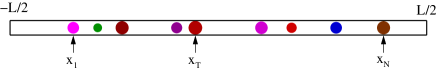
Figure 1: Cartoon of the problem considered in this study: $N$ particles are diffusing in a one-dimensional system. Particle $j$ ($j=1,...,N$) has coordinate $x_{j}$, initial coordinate $x_{j,0}$ and diffusion constant $D_{j}$. The particles cannot overtake, hence at all times we have $x_{j}<x_{j+1}$. In our analytic calculation for the two-particle case the system size is assumed to be infinite. In the stochastic simulations we assume a system of finite length $L$, with reflecting boundary conditions at $x=\pm L/2$.

Although much work has been dedicated to single-file diffusion of identical particles, fewer studies has addressed the problem of diffusion of hardcore particles with different diffusion constants. This type of system could be of interest, for instance, for protein diffusion along a DNA chain (there is a plethora of DNA binding proteins). The single-file system with different diffusion constants is illustrated in Fig. 1: The particles each have coordinates $\vec{x}=(x_{1},x_{2},...,x_{N})$ and initial coordinates $\vec{x}_{0}=(x_{1,0},x_{2,0},...,x_{N,0})$. Due to the hardcore interaction the particles cannot pass each other, and therefore retain their order at all times, i.e.,

$$-\frac{L}{2}<x_{1}<x_{2}<...<x_{N}<\frac{L}{2}.$$ (1)

where $L$ is the length of the system (and we assumed the ends of the system, at $\pm L/2$, to be reflecting). Particle $j$ has diffusion constant $D_{j}$ ($j=1,..,N$). The spatial distribution of the particles as a function of time is contained in the $N$-particle conditional PDF ${\cal P}(\vec{x},t|\vec{x}_{0})$; the equations for this quantity were given in Ref. Lizana_Ambjornsson, (with obvious modifications to account for the different diffusion constants). We are particularly interested in the dynamics of a tagged particle with coordinate $x_{\cal T}$ with initial position $x_{{\cal T},0}$, which mathematically is obtained by integrating ${\cal P}(\vec{x},t|\vec{x}_{0})$ over all coordinates and initial positions except for $x_{\cal T}$ and $x_{{\cal T},0}$. RKH ; Lizana_Ambjornsson

To our knowledge, the only studies investigating the type of single-file system described above are Refs. Aslangul_00, , Brzank2, and Jara_Gonzalves, . In Ref. Aslangul_00, the particles were assumed to be initially placed at the same position. Also, the ’annealed’ case, where the diffusion constants were randomized between the particles for each new ensemble, was considered. In Ref. Brzank2, the hydrodynamic behavior of a two-component (two different kinds of particles) single-file system with boundary injection and extraction were considered. Very recently in the mathematics literature, the asymptotic behavior for long times of a tagged particle in a single-file system with different diffusion constants was obtained for the ’quenched’ case (i.e., the diffusion constants are the same for each ensemble) for hopping dynamics on a lattice. Jara_Gonzalves

In this study we extend the results from previous studies by (i) analytically solving the problem of diffusion of two hardcore interacting particle with different diffusion constants in which the initial positions for the two particles are arbitrary, and valid for all times. The study of diffusion with arbitrary initial conditions is important in the field of single-file diffusion since in the derivation of the $t^{1/2}$-law it is assumed that the particles are initially randomly distributed. (ii) We introduce a new fast stochastic scheme tailored for interacting particle systems with different diffusion constants. (iii) For the general $N$-particle case we verify the asymptotic results obtained in Ref. Jara_Gonzalves, for long times and large $N$ using our new stochastic algorithm, and illustrate the behavior for shorter times.

II Two different hardcore interacting particles

We consider a system with two hardcore interacting particles diffusing in an infinite one-dimensional system, see Fig. 2 (top).

II.1 Equations of motion

The particles each have coordinates $\vec{x}=(x_{1},x_{2})$ and initial coordinates $\vec{x}_{0}=(x_{1,0},x_{2,0})$. The hardcore interaction prevents the particles from passing each other:

$$-\infty<x_{1}<x_{2}<\infty.$$ (2)

We denote the phase-space region spanned by coordinates $\vec{x}$ satisfying Eqs. (2) by ${\cal R}$, see Fig. 2 (bottom).

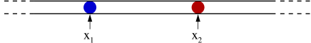
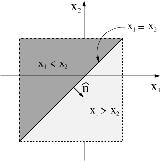
Figure 2: (top) Cartoon of the problem considered in Sec. II: two particles are diffusing in a one-dimensional system. Particle $j$ ($j=1,2$) has coordinate $x_{j}$, initial coordinate $x_{j,0}$ and diffusion constant $D_{j}$; in general $D_{1}\neq D_{2}$. The particles cannot overtake, hence at all times we have $x_{1}<x_{2}$. In our analytic calculation the system size is assumed to be infinite. In the stochastic simulations we assume a system of finite length $L$, with reflecting boundary conditions at $\pm L/2$. (bottom) Phase space region ${\cal R}$ (the darker upper area, $x_{1}<x_{2}$) for two hardcore interacting particles. For the analytic solutions ${\cal R}$ extends to $\pm\infty$.

The temporal behavior of the spatial distribution of the particles is contained in the PDF ${\cal P}(\vec{x},t|\vec{x}_{0})$ which is governed by

$$\frac{\partial{\cal P}(\vec{x},t|\vec{x}_{0})}{\partial t}=\left(D_{1}\frac{\partial^{2}}{\partial x_{1}^{2}}+D_{2}\frac{\partial^{2}}{\partial x_{2}^{2}}\right){\cal P}(\vec{x},t|\vec{x}_{0}),$$ (3)

for $\vec{x}\in{\cal R}$ [${\cal P}(\vec{x},t|\vec{x}_{0})\equiv 0$ outside ${\cal R}$] and $D_{1}$ ($D_{2}$) is the diffusion constant for particle 1 (particle 2). The initial condition is

$${\cal P}(\vec{x},0|\vec{x}_{0})=\delta(x_{1}-x_{1,0})\delta(x_{2}-x_{2,0})$$ (4)

where $\delta(z)$ is the Dirac delta-function. The fact that the particles cannot pass each other is described by

$$(D_{1}\frac{\partial}{\partial x_{1}}-D_{2}\frac{\partial}{\partial x_{2}}){\cal P}(\vec{x},t|\vec{x}_{0})|_{x_{1}=x_{2}}=0.$$ (5)

The above relation is a no flux condition for the normal component of the flux vector across the line $x_{1}=x_{2}$, see Fig. 2 (bottom): Eq. (3) can be written as a continuity equation $\partial{\cal P}/\partial t=-\vec{\nabla}\cdot\vec{{\cal J}}$, where the flux vector is $\vec{{\cal J}}=-(\hat{x}_{1}D_{1}\partial{\cal P}/\partial x_{1}+\hat{x}_{2}D_{2}\partial{\cal P}/\partial x_{2})$, and $\hat{x}_{1}$ ($\hat{x}_{2}$) is a unit vector in the $x_{1}$ ($x_{2}$) direction. The outward normal to the $x_{1}=x_{2}$ interface is (see Fig. 2) $\hat{n}=(\hat{x}_{1}-\hat{x}_{2})/\sqrt{2}$ which allows us to write Eq. (5) as $\hat{n}\cdot\vec{{\cal J}}|_{x_{1}=x_{2}}=0$. This reflecting condition guarantees that the probability in the allowed phase-space region ${\cal R}$ is conserved at all times as it should.

II.2 Solution for two-particle PDF

In order to solve the equations specified in the previous subsection we make the variable transformation:

$$X = \frac{1}{2}\left(\sqrt{\frac{D_{2}}{D_{1}}}x_{1}+\sqrt{\frac{D_{1}}{D_{2}}}x_{2}\right)$$

$$q = x_{2}-x_{1}.$$ (6)

Eqs. (3), (4) and (5) then become

$$\frac{\partial{\cal P}(X,q,t)}{\partial t} = \left(D^{X}\frac{\partial^{2}}{\partial X^{2}}+D^{q}\frac{\partial^{2}}{\partial q^{2}}\right){\cal P}(X,q,t)$$

$$\left.\frac{\partial{\cal P}(X,q,t)}{\partial q}\right|_{q=0} = 0$$

$${\cal P}(X,q,t\rightarrow 0) = \gamma\delta(X-X_{0})\delta(q-q_{0})$$ (7)

where $\gamma=(D_{1}+D_{2})/(2\sqrt{D_{1}D_{2}})$, $X_{0}=\sqrt{D_{2}/D_{1}}x_{1,0}+\sqrt{D_{1}/D_{2}}x_{2,0}$ and $q_{0}=x_{2,0}-x_{1,0}$ and we introduced the effective diffusion constants

$$D^{X} = \frac{D_{1}+D_{2}}{4}$$

$$D^{q} = D_{1}+D_{2}$$ (8)

For the case of identical diffusion constants, $D_{1}=D_{2}=D$ the equations above express the fact that the relative coordinate $q$ diffuses with a diffusion constant $2D$, whereas the center-of-mass coordinate $X$ diffuses with a diffusion constant $D/2$. Aslangul_99

Eq. (II.2) allows a product solution of the form

$${\cal P}(X,q,t)={\cal P}^{X}(X,t){\cal P}^{q}(q,t)$$ (9)

where

$${\cal P}^{X}(X,t)=\frac{\gamma}{(4\pi D^{X}t)^{1/2}}\exp(-\frac{(X-X_{0})^{2}}{4D^{X}t})$$ (10)

and the solution for ${\cal P}^{q}(q,t)$ is obtained via the method of images RKH according to

$${\cal P}^{q}(q,t) = \theta(q)\frac{1}{(4\pi D^{q}t)^{1/2}}$$ (11)

$$\times\left(\exp(-\frac{(q-q_{0})^{2}}{4D^{q}t})+\exp(-\frac{(q+q_{0})^{2}}{4D^{q}t})\right)$$

where $\theta(q)$ is the Heaviside step function, $\theta(q>0)=1$ and $\theta(q<0)=0$. Returning to our original coordinates, Eq. (9), (10) and (11) become, after some algebraic manipulations:

$${\cal P}(\vec{x},t|\vec{x}_{0}) = \theta(x_{2}-x_{1})\frac{1}{(4\pi D_{1}t)^{1/2}}\frac{1}{(4\pi D_{2}t)^{1/2}}$$ (12)

$$\times[\exp(-\frac{(x_{1}-x_{1,0})^{2}}{4D_{1}t})\exp(-\frac{(x_{2}-x_{2,0})^{2}}{4D_{2}t})$$

$$+\exp(-\frac{(x_{1}-x^{i}_{1,0})^{2}}{4D_{1}t})\exp(-\frac{(x_{2}-x^{i}_{2,0})^{2}}{4D_{2}t})]$$

where the effective image initial positions are

$$x^{i}_{1,0} = \frac{D_{2}-D_{1}}{D_{1}+D_{2}}x_{1,0}+\frac{2D_{1}}{D_{1}+D_{2}}x_{2,0}$$

$$x^{i}_{2,0} = \frac{2D_{2}}{D_{1}+D_{2}}x_{1,0}+\frac{D_{1}-D_{2}}{D_{1}+D_{2}}x_{2,0}$$ (13)

Notice that we have $x^{i}_{2,0}-x^{i}_{1,0}=-(x_{2,0}-x_{1,0})$, i.e. the distance between the image initial positions is the same as the distance between the initial positions. Eq. (II.2) is a non-trivial extension of the image positions for identical particles or for a system where the particles initially start out at the same point in space: For $D_{1}=D_{2}$ we have $x^{i}_{1,0}=x_{2,0}$ and $x^{i}_{2,0}=x_{1,0}$ as it should. Fisher_84 For the case $x_{1,0}=x_{2,0}=0$ the results above reduce to the results obtained in Ref. Aslangul_00, . Note that, in contrast, when $D_{1}\neq D_{2}$ and $x_{1,0}\neq x_{2,0}$ the image initial positions, Eq. (II.2), depend on $D_{1}$ and $D_{2}$.

It is interesting to compare the above result for ${\cal P}(\vec{x},t|\vec{x}_{0})$ to that of a Bethe-ansatz SC ; Batchelor_07 . It is straightforward to show that Eq. (12) can be written:

$${\cal P}(\vec{x},t|\vec{x}_{0}) = \theta(x_{2}-x_{1})\int_{-\infty}^{\infty}\frac{dk_{1}}{2\pi}\int_{-\infty}^{\infty}\frac{dk_{2}}{2\pi}$$ (14)

$$e^{-D_{1}k_{1}^{2}t}e^{-D_{2}k_{2}^{2}t}e^{-ik_{1}x_{1,0}}e^{-ik_{2}x_{2,0}}$$

$$\times[e^{ik_{1}x_{1}}e^{ik_{2}x_{2}}+g(k_{1},k_{2},x_{1},x_{2})e^{ik_{2}x_{1}}e^{ik_{1}x_{2}}]$$

where

$$g(k_{1},k_{2},x_{1},x_{2})=\exp[\frac{D_{1}-D_{2}}{D_{1}+D_{2}}(k_{1}+k_{2})(x_{2}-x_{1})]$$ (15)

We note that Eq. (14) has the form of a Bethe ansatz SC , where the “scattering coefficient” $g$ depends on $x_{1}$ and $x_{2}$ (in the standard Bethe ansatz the scattering coefficient only depends on $k_{1}$ and $k_{2}$); the standard Bethe-ansatz satisfies the equations of motion and the boundary conditions for fixed $k_{1}$ and $k_{2}$; in contrast, the solution above does not - it is only after the integrations over $k_{1}$ and $k_{2}$ are performed [with the appropriate $x_{1}$ and $x_{2}$ dependent “mixing” of $k_{1}$ and $k_{2}$ from the 2nd term in Eq. (14)] that the correct solution for ${\cal P}(\vec{x},t|\vec{x}_{0})$ is obtained. For the case of identical diffusion constants $D_{1}=D_{2}=D$ the mixing of $k_{1}$ and $k_{2}$ in $g$ is absent and we have $g=1$ in agreement with previous studies. Lizana_Ambjornsson

II.3 Tagged particle PDF

By integrating the two-particle PDF we obtain the tagged particle PDF. The tagged PDF (for fixed initial positions) for particle 1 is $\rho_{1}(x_{1},t|\vec{x}_{0})=\int_{x_{1}}^{\infty}dx_{2}{\cal P}(\vec{x},t|\vec{x}_{0})$. Explicitly, using Eq. (12), we have:

$$\rho_{1}(x_{1},t|\vec{x}_{0}) = \frac{1}{(4\pi D_{1}t)^{1/2}}\exp(-\frac{(x_{1}-x_{1,0})^{2}}{4D_{1}t})$$ (16)

$$\times\frac{1}{2}{\rm erfc}(\frac{x_{1}-x_{2,0}}{\sqrt{4D_{2}t}})$$

$$+\frac{1}{(4\pi D_{1}t)^{1/2}}\exp(-\frac{(x_{1}-x^{i}_{1,0})^{2}}{4D_{1}t})$$

$$\times\frac{1}{2}{\rm erfc}(\frac{x_{1}-x^{i}_{2,0}}{\sqrt{4D_{2}t}})$$

where ${\rm erfc}(z)=1-{\rm erf}(z)$ is the complementary error function, with ${\rm erf}(z)=(2/\sqrt{\pi})\int_{0}^{z}dy\exp(-y^{2})$ being the error function ABST and $x_{1,0}^{i}$ and $x_{2,0}^{i}$ are given in Eq. (II.2). The tagged particle PDF for particle 2 $\rho_{2}(x_{2},t|\vec{x}_{0})=\int_{-\infty}^{x_{2}}dx_{1}{\cal P}(\vec{x},t|\vec{x}_{0})$ is obtained by the replacements $x_{1}\leftrightarrow-x_{2}$, $x_{1,0}\leftrightarrow-x_{2,0}$, $x^{i}_{1,0}\leftrightarrow-x^{i}_{2,0}$, and $D_{1}\leftrightarrow D_{2}$ in Eq. (16). We point out that Eq. (16) does not give an MSD which scales with time as $t^{1/2}$ (see Introduction); it is only in the limit of a large number of hardcore interacting particles that $\rho_{j}(x_{j},t|\vec{x}_{0})$ (with an additional average over the initial position of non-tagged particles), for a center particle, becomes a Gaussian with a width that scales as the square root of time, see next section.

A limit not accessible through previous approaches Fisher_84 ; Aslangul_00 is that where one of the particles is immobile $D_{2}=0$: setting $x_{20}=0$ for convenience and taking the limit $D_{2}\rightarrow 0$ Eq. (16) becomes

$$\rho_{1}(x_{1},t|\vec{x}_{0})|_{D_{2}=0} = \theta(-x_{1})\frac{1}{(4\pi D_{1}t)^{1/2}}$$ (17)

$$\times[\exp(-\frac{(x_{1}-x_{1,0})^{2}}{4D_{1}t})+\exp(-\frac{(x_{1}+x_{1,0})^{2}}{4D_{1}t})],$$

in agreement with the diffusion of a particle near a reflecting wall as it should. We have above used the fact that ${\rm erf}(\pm\infty)=\pm 1$.

In Fig. 3 we illustrate the results for the tagged particle PDFs as given in Eq. (16). We compare to stochastic simulations using a new stochastic algorithm described in Appendix A. In the simulation we assume a finite box; the main effect of the finite box (with reflecting conditions) is to modify the long-time limit (i.e. for $t\gg L^{2}/D_{j}$), to the following equilibrium PDFs: Lizana_Ambjornsson

$$\rho^{\rm eq}(x_{1}) = \frac{2}{L^{2}}\left(\frac{L}{2}-x_{1}\right),$$

$$\rho^{\rm eq}(x_{2}) = \frac{2}{L^{2}}\left(\frac{L}{2}+x_{2}\right)$$ (18)

The results given in Eq. (II.3) is obtained by direct integration of the two-particle equilibrium PDF $P^{\rm eq}(x_{1},x_{2})=2\theta(x_{2}-x_{1})/L^{2}$. The equilibrium results are independent on $D_{1}$ and $D_{2}$ as it should. In Fig. 3 we illustrate the result of a Gillespie simulation using $n_{\rm ens}=50000$ ensembles on a lattice with $M=500$ lattice points, and compare to the PDF Eq. (16) as well as the equilibrium PDF, Eq. (II.3). We notice excellent agreement within the limit of applicability.

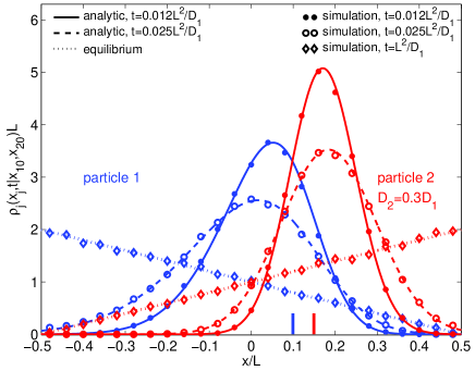
Figure 3: Tagged particle PDF $\rho_{j}(x_{j},t|\vec{x}_{0})$ for two hardcore interacting particles ($j=1,2$). The solid and dashed leftmost (blue) [rightmost (red)] curves corresponds to the tagged particle PDF for particle 1 [particle 2] at different times as given in Eq. (16). The ratio of the diffusion constants is $D_{2}/D_{1}=0.3$. The symbols correspond to the results of the Gillespie simulation, ensemble-averaged over $n_{\rm ens}=50000$ ensembles for $M=500$ lattice sites; the data was binned into 25 bins. The vertical bars at the bottom of the figure corresponds to the initial positions for the two particles ($x_{1,0}=0.10L$ and $x_{2,0}=0.15L$). For long time $t>L^{2}/D$ the equilibrium is reached - the dashed lines correspond to the analytic result as given in Eq. (II.3).

It remains a challenge to generalize the results in this section to the $N$-particle case and arbitrary times. In the next section we perform stochastic simulations for $N$ particles and verify the asymptotic results in Ref. Jara_Gonzalves, for long times and $N$ large.

III $N$ different hardcore interacting particles

For $N$ identical point particles we have the standard result $\langle(x_{\cal T}-x_{{\cal T},0})^{2}\rangle=(1/\varrho)(4Dt/\pi)^{1/2}$ for the MSD of a tagged particle, where $\varrho=N/L$ is the concentration of particles ($N,L\rightarrow\infty$ with $\varrho$ kept fixed). HA ; LE ; Lizana_Ambjornsson For single-file particles with different diffusion constants very recent results show that the motion for a tagged particle stochastically jumping on a lattice (exponential waiting time between jumps) is a fractional Brownian motion (so that the PDF is Gaussian). Jara_Gonzalves The MSD was in Ref. Jara_Gonzalves, shown to take the same form as for identical diffusion constant but where $D$ above is replaced by an effective diffusion constant, i.e., we have:

$$\langle(x_{\cal T}-x_{{\cal T},0})^{2}\rangle=\kappa\left(\frac{4D_{\rm eff}t}{\pi}\right)^{1/2}$$ (19)

with the prefactor

$$\kappa=a\frac{1-f}{f}$$ (20)

where $f=N/M$, $M$ is the number of lattice points and $a$ the lattice spacing ($N,M\rightarrow\infty$ with $f$ fixed). In the continuum limit (lattice spacing $a\rightarrow 0$) we get the point-particle result $\kappa=1/\varrho$. In the continuum limit but with finite-sized particles we have, as in Ref. Lizana_Ambjornsson, , that $\kappa=(1-\varrho\Delta)/\varrho$, where $\Delta$ is the size of the particles. The effective diffusion constant appearing in Eq. (19) is obtained by averaging the friction coefficients (inverse of diffusion constants) according to:

$$\frac{1}{D_{\rm eff}}={\rm lim}_{N\rightarrow\infty}\frac{1}{N}\sum_{i=1}^{N}\frac{1}{D_{i}}$$ (21)

provided the limit on the right-hand side exists. Footnote1 The result above is obtained for the (realistic) ’quenched’ case, i.e., $D_{i}$ are kept the same for all the ensembles. The results above are thus stronger than the results in Ref. Aslangul_00, where the ’annealed’ case, i.e. for each ensemble the diffusion constants are reshuffled between the particles, was studied. We also point out that the results above are valid for an initial equilibrium density of particles, whereas the results in Ref. Aslangul_00, are limited to the case that all particles are initially placed at the same point in space.

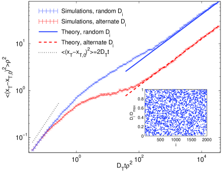
Figure 4: Mean square displacement for a tagged particle in the center of a single-file system with different diffusion constants. The upper (blue online) marks show the simulation results for a system where the diffusion constants are ’quenched’ and random with $0.01D_{\rm max}\leq D_{i}\leq D_{\rm max}$ (the inset shows the diffusion constants used). The lower (red online) marks are the results for an alternating sequence of diffusion constants: $D_{1}=D_{\rm max}$,$D_{2}=0.01D_{\rm max}$,$D_{3}=D_{\rm max}$, $D_{4}=0.01D_{\rm max}$ etc. For both cases the tagged particle’s diffusion constant $D_{\cal T}$ was set equal to $D_{\rm max}$. The solid blue and dashed red line are the analytic result as given in Eqs. (19)-(21). In all simulations the tagged particle was initially placed at the center lattice point and the non-tagged particles then randomly positioned to the left and right of the tagged particle. The errorbars are the standard errors. The following parameters were used: $M=10001$, $N=2001$ and the number of ensembles $n_{\rm ens}=3200$. Without loss of generality, we set $a=1$ and $D_{\cal T}=1$ (i.e., $a$ and $D_{\cal T}$ determine the units of length and time in the problem) in all simulations. Particle $1001$ was taken to be tagged.

In Fig. 4 we show results of stochastic simulations for $N=2001$ particles, with the middle particle (particle number $1001$) being tagged. The tagged particle is initially placed at the center lattice point and the remaining particles are randomly positioned (avoiding multiply occupied lattice sites Bebbington ) to the left and right of the tagged particle for each ensemble. The details of our stochastic scheme is presented in Appendix A. Two cases are presented: the upper (blue) marks shows simulations for the case of random ’quenched’ distribution of diffusion constants drawn between $0.01D_{\max}$ and $D_{\rm max}$. The tagged particle diffusion constant $D_{\cal T}$ was set to $D_{\rm max}$, and the diffusion constants used are shown in the inset in the figure. The lower (red) marks represent results for an alternating set of diffusion constants: the first particle has diffusion constant $D_{\rm max}$, the second particles has $0.01D_{\rm max}$ the third $D_{\rm max}$ etc. The tagged particle has diffusion constant $D_{\rm max}$. For short times, $t\ll 1/(\varrho^{2}D_{\cal T})$, we see that the case of ’quenched’ random and alternating diffusion constants give the same MSD (the tagged particle has a diffusion constant equal to $D_{\rm max}$ in both cases). There has been few collisions between particles and the MSD is proportional to $t$, see Fig. 4. The MSD in the short-time regime is slightly smaller than that of a free particle $\langle(x_{\cal T}-x_{{\cal T},0})^{2}\rangle=2D_{\cal T}t$ [dotted line], simply due to the fact that in some ensembles the tagged particle will initially have a non-tagged particle at a neighbouring lattice site (every fifth lattice site will on average contain a particle in the simulations in the figure). For long times, $t\gg 1/(\varrho^{2}D_{\rm eff})$, there is a cross-over to a single-file regime with the MSD proportional to $t^{1/2}$. We notice an excellent agreement with the stochastic simulations and the prediction in Eq. (19)-(21) [solid blue and dashed red line] for long times. We point out that the average diffusion constants [$(1/N)\sum_{i=1}^{N}D_{i}$ ] for the two cases above are very close (more precisely, the two cases converge to the same average diffusion constant for $N\rightarrow\infty$); Fig. 4 thus clearly illustrates that it is the average friction coefficient which determine the long-time behavior for the system rather than the average diffusion constant. For very long times (beyond the time window in Fig. 4) and finite $L$, the equilibrium PDF for the tagged particle should be reached, see Ref. Lizana_Ambjornsson, for an explicit expression.

IV Summary and outlook

In this study we have investigated the (single-file) dynamics of hardcore interacting particles with different diffusion constants diffusing in a one-dimensional system. For the two particle case we obtained an analytic result for the conditional PDF (for arbitrary initial particle positions and all times), from which we calculated the tagged particle PDF, see Eq. (16). For the general $N$-particle case an asymptotic expression for the mean square displacement of a tagged particle for long times was given, Eq. (19), and excellent agreement was found with our new computationally efficient stochastic simulation technique based on the Gillespie algorithm.

It will be interesting to see whether it is possible to generalize our two-particle PDF to $N$ particles with different diffusion constants, in order to access the full time behavior, and thus going beyond the asymptotic results in Ref. Jara_Gonzalves, . We point out that the $N$ particle results given in this study assumed the mean friction constant to be finite; we are currently considering the case of a distribution of friction constants with diverging first moment.

The problem studied here, the dynamics of interacting species of different kinds, shares many features with the dynamical behaviour of cellular (and other biological) systems where heterogeneity and interactions are important factors. We hope that our study will inspire to further studies of many-body biology effects in living systems.

V Acknowledgments

We thank Milton Jara for sending an early version of Ref. Jara_Gonzalves, and for helpful correspondence. We are grateful for discussions with Ophir Flomenbom. T.A. acknowledges the support from the Knut and Alice Wallenberg Foundation. Part of this research was supported by the NSF under grant CHE0556268, and the Danish National Research Foundation via a grant to MEMPHYS. Computing time was provided by the Danish Center for Scientific Computing at the University of Southern Denmark.

Appendix A New efficient stochastic algorithm based on the Gillespie algorithm

Stochastic simulations using the Gillespie algorithm DG1 ; DG2 ; DG3 is a convenient technique for generating stochastic trajectories for interacting particles. Briefly, we consider hopping of $N$ particles on a lattice with $M$ lattice sites. The dynamics is governed by the ‘reaction’ probability density (rPDF)

$$P(\tau,\mu)=k_{\mu}\exp(-\sum_{\nu=0}^{2N-1}k_{\nu}\tau)$$ (22)

where $\tau$ is the waiting time between jump events and $k_{\mu}$ are the jump rates. There are $2N$ jump rates for the process considered here ($\mu=0,...,2N-1$): the rate for particle $1$ to $N$ jumping to the left and right respectively. We enumerate these rates such that $k_{2i-2}$ is the rate for particle $i$ jumping to the left, and $k_{2i-1}$ is the rate for particle $i$ jumping to the right, see Fig. 5. For the case that a particle have no neighbors nor are at the end lattice points we set $k_{\mu}=k_{\mu}^{f}$ where $k_{\mu}^{f}$ are the “free” hop rates.

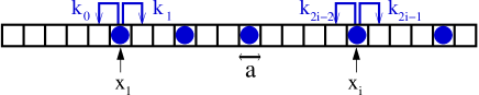
Figure 5: Schematic illustration of the lattice on which $N$ particles jump in the Gillespie simulation. The number of lattice sites are denoted by $M$ and the lattice spacing is $a$. Particle $i$ jumps to the left (right) with rate $k_{2i-2}$ ($k_{2i-1}$). Note that these rates change during the simulation: if particle 1 is at the leftmost site then we impose the reflecting condition $k_{1}=0$. Similarly if particle $N$ is at the rightmost site we have $k_{2N-1}=0$. If particle $i$ and $i+1$ are at neighboring sites we set $k_{2i-1}=k_{2i}=0$ due to the hardcore repulsion. For the remaining configurations we have that the hop rates take the “free” values: $k_{\mu}=k_{\mu}^{f}$.

For the case that particle 1 (particle $N$) is at the leftmost (rightmost) lattice point we have the reflecting condition $k_{1}=0$ ($k_{2N-1}=0$). If two particles are at neighboring sites the hardcore repulsion requires the right (left) rate for the leftmost (rightmost) particle equals zero, i.e. if particle $i$ and $i+1$ are at neighboring site we set $k_{2i-1}=k_{2i}=0$. Jump rates that are not set to zero are equal to their “free” hop rates. Thus, a stochastic time series is generated through the steps: (1) place the particles at their initial positions; (2) From the rPDF given in Eq. (22) we draw the random numbers $\tau$ (waiting time) and $\mu$ (which particle to move and in what direction); (3) Update the position of the chosen particle, the time $t$ and the rates $k_{j}$ for the new configuration and return to (2); (4) The loop (1)-(3) is repeated until $t\geq t_{\rm stop}$, where $t_{\rm stop}$ is the stop time for the simulation. This procedure produces a stochastic time series for $0\leq t\leq t_{\rm stop}$. If steps (1)-(4) are repeated $n_{\rm ens}$ times one obtains a histogram of particle positions (at specified times). The ensemble averaged results of a Gillespie time series is equivalent to the solution of a master equation incorporating the rates given above; DG1 ; DG2 see for instance Refs. Golinelli_06, or SC, for the explicit expression for this master equation. In the limit $a\rightarrow 0$ with fixed diffusion constants $D_{i}=(k^{f}_{2i-2}+k^{f}_{2i-1})a^{2}/2$ the master equation approaches the diffusion equation (assuming no drift, i.e. that $k^{f}_{2i-2}=k^{f}_{2i-1}$) as specified in section II for an infinite system.

In the two subsequent subsections we consider two different methods for generating a stochastic time series for the type of dynamics described above: (A) the direct method and, and our new approach (B) the trial-and-error method. We find that the latter method is superior in computational speed whenever the fraction of occupied lattice sites is not close to one.

A.1 (A) The direct method

Let us now review the “direct method” used for obtaining a stochastic time series using the rPDF as given in Eq. (22). Briefly, the direct method as applied to the present type of system involves the following steps DG1 ; DG2 ; DG3

1. Place the $N$ particles at their initial positions and assign free hop rates $k_{\mu}^{f}$.

2. Draw two random numbers $r_{1}$ and $r_{2}$ ($0<r_{1},r_{2}<1$)

3. The waiting time is obtained from the first random number as:

   $$\tau=\frac{1}{\sum_{\mu=0}^{2N-1}k_{\mu}}\log\left(\frac{1}{r_{1}}\right)$$ (23)

4. The ‘reaction’ $\mu$ is determined by using $r_{2}$ to determine the $\mu$ which satisfies

   $$\sum_{\nu=0}^{\mu-1}k_{\nu}<r_{2}\sum_{\nu=0}^{2N-1}k_{\nu}\leq\sum_{\nu=0}^{\mu}k_{\nu}$$ (24)

5. Use the obtained $\mu$ and $\tau$ to update the particle positions $X_{i}(t)$ and the time. After the chosen particle has been moved, check the local environment for the particle and if necessary update the rate constants $k_{\mu}$ accordingly ($k_{\mu}$ is either equal to $k_{\mu}^{f}$ or 0).

6. Return to step (2).

This procedure produces a stochastic time series $X_{i}(t)$ for the particle positions. If steps (1)-(6) are repeated $n_{\rm ens}$ times ($n_{\rm ens}$ ensembles) one obtains a histogram of particle positions (at specified times).

The direct method as applied to the present type of system is computationally slow, since at each step the sum of all rate constants has to be recalculated.

A.2 (B) The trial-and-error method

In this subsection we present a new method for generating a time series according to the rPDF as given in Eq. (22); we call this method the trial-and-error method.

1. Generate the partial sums of the free rate constants

   $$p_{0} = 0$$

   $$p_{\mu} = \sum_{\nu=0}^{\mu-1}k_{\nu}^{f},\ \mu=1,...,2N$$ (25)

2. Generate an initial configuration of particle positions.

3. Set the waiting time equal to zero, $\tau=0$.

4. Draw a random number $r_{1}$ ($0<r_{1}<1$). The waiting time is updated according to:

   $$\tau\rightarrow\tau+\frac{1}{p_{2N}}\log\left(\frac{1}{r_{1}}\right)$$ (26)

5. Draw a random number $r_{2}$ ($0<r_{2}<1$). A trial ‘reaction’ is determined by the $\mu$ which satisfies

   $$p_{\mu}<r_{2}p_{2N}\leq p_{\mu+1}$$ (27)

6. Check if there is a reflecting wall or neighboring particle preventing the ‘reaction’ $\mu$ from occurring, if so return to step (4). If $\mu$ is allowed then update the particle positions and the time.

7. Return to step (3).

The scheme above produces a stochastic time series $X_{i}(t)$, and if steps (2)-(7) are repeated $n_{\rm ens}$ times ($n_{\rm ens}$ ensembles) one obtains a histogram of particle positions; note that step (1) does not have to repeated for each ensemble. An efficient method for performing the search for the $\mu$ satisfying the inequality in Eq. (27) is presented in Appendix B. Notice that in the scheme above one does not have to update the $k_{\mu}$ at each time step, since we are only using the free rate constants $k_{\mu}^{f}$ (which are fixed at all times) in the present scheme, nor do we need to perform a sum over all rate constant at each time step. The only price we have to pay compared to the direct method is the rejection step (6), which may cause us to repeat steps (4) and (5) several times. However, whenever the fraction of occupied lattice points is not close to one (or more precisely, essentially whenever the occupation fraction is such that we can find an allowed reaction in less than $N$ steps) we expect that the trial-and-error method is faster than the direct method. A proof that the direct and the trial-and-error methods are mathematically equivalent is presented in Appendix C.

Appendix B Fast method for determining $\mu$ from Eq. (27)

In this appendix we give a simple, yet fast, algorithm for determining the $\mu$ satisfying Eq. (27). We start by noticing that if all $k_{\mu}^{f}$ are identical then we can directly satisfy Eq. (27) by choosing $\mu=[2Nr_{2}]$, where $[z]$ gives the largest integer smaller than $z$. The algorithm below uses this fact to directly find the correct $\mu$ for identical rate constants; for non-identical rate constants we expect the number of attempts before the correct $\mu$ is found to scale not worse than $\log N$ (see below). The algorithm is:

1. Initialize the two “boundary” parameters $\mu^{\rm left}$ and $\mu^{\rm right}$ to $\mu^{\rm left}=0$ and $\mu^{\rm right}=2N$. Also, introduce $p^{\rm left}$ and $p^{\rm right}$ which are initialized to the largest and smallest of the partial sums, i.e. we set initially $p^{\rm left}=p_{0}=0$ and $p^{\rm right}=p_{2N}$, see Eq. (1).

2. Make a guess for $\mu$ using the formula

   $$\mu_{\rm guess}=[\frac{r_{2}p_{2N}-p^{\rm left}}{p^{\rm right}-p^{\rm left}}(\mu^{\rm right}-\mu^{\rm left})+\mu_{\rm left}].$$ (28)

3. Check if the guess value for $\mu$ satisfies Eq. (27), if so terminate the loop.

4. If the guess value for $\mu$ does not satisfy Eq. (27) we separate between the cases: (a) if $r_{2}p_{2N}\leq p_{\mu_{\rm guess}}$ then move the right boundary parameters by changing $\mu^{\rm right}\rightarrow\mu_{\rm guess}$ and $p^{\rm right}\rightarrow p_{\mu_{\rm guess}}$; (b) if $r_{2}p_{2N}>p_{\mu_{\rm guess}+1}$ then move the left boundary parameters by changing $\mu^{\rm left}\rightarrow\mu_{\rm guess}+1$ and $p^{\rm left}\rightarrow p_{\mu_{\rm guess}+1}$. Then return to step (2).

The algorithm above will narrow down the search to a smaller and smaller segment along the $\mu$-axis, until we manage to obtain the correct $\mu$. The initial guess will always be $\mu_{\rm guess}=[2Nr_{2}]$, see Eq. (28), and hence for identical free rate constants $k_{0}^{f}=k_{1}^{f}=...=k_{2N-1}^{f}$ the algorithm above directly finds the correct $\mu$. To argue for the maximally $\log N$-scaling for the number of iterations note that if we had chosen $\mu_{\rm guess}=[(\mu^{\rm right}-\mu^{\rm left})/2]$ in the algorithm then the number of steps to find the correct $\mu$ would be maximally $[1+\log_{2}N]$. The algorithm above should perform better than this because the values of $\mu_{\rm guess}$ should approach the correct $\mu$ faster.

Appendix C Proof of equivalence of the direct method and the trial-and-error method

Let us finally prove that indeed the trial-and-error method is equivalent to the Gillespie rPDF, Eq. (22). More precisely we prove that the successful ‘reaction’ probability density function $P(\tau,\mu)$ agrees with Eq. (22). Let us first define a trial-and-error relaxation time as

$$\tau_{\rm TE}=\frac{1}{\sum_{\mu=0}^{2N-1}k_{\mu}^{f}}$$ (29)

and we note that for each (successful or unsuccessful) attempt we draw a waiting time from the PDF:

$$\rho_{\rm TE}(\tau)=\frac{1}{\tau_{\rm TE}}e^{-\tau/\tau_{\rm TE}}$$ (30)

see step (4) in the trial-and-error Gillespie scheme. To construct $P(\tau,\mu)$ within the trial-and-error method we have to wait for a successful attempt. We therefore separate between the following (mutually exclusive) events:

• success on the first attempt: the probability for this is

  $$\sigma_{0}=q=\frac{\sum_{\mu=0}^{2N-1}k_{\mu}}{\sum_{\mu=0}^{2N-1}k_{\mu}^{f}}=\frac{\tau_{\rm TE}}{\tau_{G}}$$ (31)

  where $\tau_{G}=1/[\sum_{\mu=0}^{2N-1}k_{\mu}]$ is the relaxation time for a successful event.

• one failed attempt, then success: the probability for this is $\sigma_{1}=q(1-q)$.

• …..

• $m$ failed attempts and then success: the probability is $\sigma_{m}=q(1-q)^{m}$.

• …..

Given one of the above events the probability that reaction $\mu$ occurs is

$$\rho_{\mu}=\frac{k_{\mu}}{\sum_{\nu=0}^{2N-1}k_{\nu}}=k_{\mu}\tau_{G}$$ (32)

The successful rPDF thus becomes

$$P(\tau,\mu) = \rho_{\mu}\sigma_{0}\rho_{\rm TE}(\tau)$$ (33)

$$+\rho_{\mu}\sigma_{1}\int_{0}^{\tau}d\tau_{1}\rho_{\rm TE}(\tau_{1})\rho_{\rm TE}(\tau-\tau_{1})$$

$$+\rho_{\mu}\sigma_{2}\int d\tau_{1}d\tau_{2}\rho_{\rm TE}(\tau_{1})$$

$$\times\rho_{\rm TE}(\tau_{2}-\tau_{1})\rho_{\rm TE}(\tau-\tau_{2})+..$$

The first term is the PDF for a successful move of type $\mu$ on the first attempt. The second term is the PDF for a successful move of type $\mu$ on the second attempt, and is obtained by considering the waiting time density to first make an unsuccessful attempt at time $\tau_{1}$ followed by a successful attempt at time $\tau$; since $\tau_{1}$ can take any value between $0$ and $\tau$ we must integrate over this interval. Similar arguments give expressions for higher order terms. In order to express the result given in Eq.(33) in closed form we make a Laplace-transform which gives:

$$P(u,\mu) = \int_{0}^{\infty}du\ e^{-u\tau}P(\tau,\mu)=\rho_{\mu}\sigma_{0}\rho_{\rm TE}(u)$$ (34)

$$+\rho_{\mu}\sigma_{1}[\rho_{\rm TE}(u)]^{2}+\rho_{\mu}\sigma_{2}[\rho_{\rm TE}(u)]^{3}+..$$

$$= \rho_{\mu}\sum_{n=1}^{\infty}\sigma_{n-1}[\rho_{\rm TE}(u)]^{n}$$

$$= \rho_{\mu}q\rho_{\rm TE}(u)\sum_{n=0}^{\infty}[(1-q)\rho_{\rm TE}(u)]^{n}$$

where $\rho_{\rm TE}(u)=1/(1+u\tau_{\rm TE})$ is the Laplace-transform of Eq. (30). Using the fact that the series in Eq. (34) is a geometric series $\sum_{n=0}^{\infty}a^{n}=1/(1-a)$, the explicit expression for $\rho_{\rm TE}(u)$ and Eq. (31), we finally find:

$$P(u,\mu)=\frac{\rho_{\mu}}{1+u\tau_{\rm TE}/q}=\frac{k_{\mu}}{\tau_{\rm G}^{-1}+u}$$ (35)

In the time domain this is the same as Eq. (22), which thereby completes the proof.

References

- (1) L. Luby-Phelps, Int. Rev. Cytol. 192, 189 (2000).
- (2) R.J. Ellis and A.P. Milton, Nature 425, 27 (2003).
- (3) A. L. Hodgkin and R. D. Keynes, J. Physiol. (London) 128, 61 (1955).
- (4) P. M. Richards, Phys. Rev. B 16, 1393 (1977).
- (5) V. Kukla, J. Kornatowski, D. Demuth, I. Girnus, H. Pfeifer, L. Rees, S. Schunk, K. Unger, and J. Kärger, Science 272, 702 (1996).
- (6) O.G. Berg, R.B. Winter and P.H. von Hippel, Biochemistry 20, 6929 (1981).
- (7) S.E. Halford, J.F. Marko, Nucleic Acids Research 32, 3040 (2004).
- (8) M.A. Lomholt, T. Ambjörnsson and R. Metzler, Phys. Rev. Lett. 95, 260603 (2005).
- (9) G. Coupier, M. S. Jean and C. Guthmann, Phys. Rev. E 73, 031112 (2006).
- (10) C. Lutz, M. Kollmann and C. Bechinger, Phys. Rev. Lett. 92, 026001 (2004).
- (11) Q. H. Wei, C. Bechinger, P. Leiderer, Science 287, 625 (2000).
- (12) T. E. Harris, J. Appl. Prob. 2(2), 323 (1965).
- (13) D. G. Levitt, Phys. Rev. A 6, 3050 (1973).
- (14) H. van Beijeren, K.W. Kehr and R. Kutner, Phys. Rev. B 28, 5711 (1983).
- (15) K. Hahn and J. Kärger, J. Phys. A 28, 3061 (1995).
- (16) R. Arratia, Ann. Prob. 11, 362 (1983).
- (17) C. Aslangul, Europhys. Lett. 44, 284 (1998).
- (18) F. Marchesoni and A. Taloni, Phys. Rev. Lett. 97, 106101 (2006).
- (19) M. Kollmann, Phys. Rev. Lett. 90, 180602 (2003).
- (20) M.D. Jara and C. Landim, Ann. I.H. Poincaré - PR 42, 567 (2006).
- (21) A.Y. Grosberg and A.R. Khokhlov, Statistical Physics of Macromolecules, AIP Press, New York (1994).
- (22) R. Shusterman, S. Alon, T. Gavrinyov and O. Krichevsky, Phys. Rev. Lett 92, 048303 (2004).
- (23) R. Metzler and J. Klafter, Phys. Rep. 339, 1 (2000).
- (24) R. Metzler and J. Klafter, J. Phys. A 37, R161 (2004).
- (25) L. Lizana and T.Ambjörnsson, Phys. Rev. Lett. 100, 200601 (2008).
- (26) C. Rödenbeck, J. Kärger and K. Hahn, Phys. Rev. E 57, 4382 (1998).
- (27) C. Aslangul, J. Phys. A 33, 851 (2000).
- (28) A. Brzank and G.M. Schütz, J. Stat. Mech: Theory and Experiment P08028 (2007); E-print arXiv:cond-mat/0611702.
- (29) M. Jara and P. Gonçalves, J. Stat. Phys. (in press); E-print arXiv:0804.3018.
- (30) C. Aslangul, J. Phys. A 32, 3993 (1999).
- (31) M.E. Fisher, J. Stat. Phys. 34, 667 (1984).
- (32) G. M. Schutz, J. Stat. Phys. 88, 427 (1997).
- (33) M.T. Batchelor, Phys. Today 60, 36 (2007).
- (34) Milton Abramowitz and Irene A. Stegun, Handbook of Mathematical Functions with Formulas, Graphs, and Mathematical Tables, (Dover, New York, 1964).
- (35) The mathematical proof of Eqs. (19)-(21) also requires the average friction for the particles to the left of the tagged particle should equal the average friction to the right, i.e. that , where () is the number of particles to the left (right) of the tagged particle.
- (36) A.C. Bebbington, Appl. Stat. 24, 136 (1975).
- (37) D. Gillespie, J. Comput. Phys. 22, 403 (1976).
- (38) D. Gillespie, J. Chem. Phys. 115, 1716 (2001).
- (39) D.T. Gillespie, Ann. Rev. Phys. Chem. 58, 35 (2007).
- (40) O. Golinelli and K. Mallick, J. Phys. A: Math. Gen. 39, 12679 (2006).