Uniqueness Results for Nonlocal Hamilton-Jacobi Equations

Abstract.

We are interested in nonlocal Eikonal Equations describing the evolution of interfaces moving with a nonlocal, non monotone velocity. For these equations, only the existence of global-in-time weak solutions is available in some particular cases. In this paper, we propose a new approach for proving uniqueness of the solution when the front is expanding. This approach simplifies and extends existing results for dislocation dynamics. It also provides the first uniqueness result for a Fitzhugh-Nagumo system. The key ingredients are some new perimeter estimates for the evolving fronts as well as some uniform interior cone property for these fronts.

1. Introduction

In this article, we are interested in uniqueness results for different types of problems which can be written as nonlocal Hamilton-Jacobi Equations of the following form:

$$u_{t}=c[{11}_{\{u\geq 0\}}](x,t)|Du|\quad\hbox{in }{\mathbb{R}}^{N}\times(0,T)\;,$$ (1.1)

$$u(x,0)=u_{0}(x)\quad\hbox{in }{\mathbb{R}}^{N}\;,$$ (1.2)

where $T>0$, the solution $u$ is a real-valued function, $u_{t}$ and$Du$ stand respectively for its time and space derivatives and ${11}_{A}$ is the indicator function of a set $A$. Finally $u_{0}$ is a bounded, Lipschitz continuous function.

For any indicator function $\chi$ or more generally for any $\chi\in L^{\infty}$ with $0\leq\chi\leq 1$ a.e., the function $c[\chi]$ depends on $\chi$ in a nonlocal way and, in the main examples we have in mind, it is obtained from $\chi$ through a convolution type procedure (either only in space or in space and time). In particular, in our framework, despite the fact that $\chi$ has no regularity neither in $x$ nor in $t$, $c[\chi]$ will be always Lipschitz continuous in $x$; on the contrary we impose no regularity with respect to $t$. More precisely we always assume in the sequel that, for any $\chi$, the velocity $c=c[\chi]$ satisfies

(H1) For all $x\in{\mathbb{R}}^{N}$, $t\mapsto c(x,t)$ is measurable and there exist ${C},{\underline{c}},{\overline{c}}>0$ such that, for all $x,y\in{\mathbb{R}}^{N}$ and $t\in[0,T],$

$$|c(x,t)-c(y,t)|\leq{C}|x-y|,$$

$$0<{\underline{c}}\leq c(x,t)\leq{\overline{c}}.$$ (1.3)

We will come back to this assumption later on.

To give a first flavor of our main uniqueness results, we can point out the following key facts: Equation (1.1) can be seen as the “level-set approach”-equation associated to the motion of the front $\Gamma_{t}:=\{x:u(x,t)=0\}$ with the nonlocal velocity $c[{11}_{\{u(\cdot,t)\geq 0\}}].$ However, in the non-standard examples we consider, it is not only a nonlocal but also non-monotone “geometrical” equation; by non-monotone we mean that the inclusion principle, which plays a central role in the “level-set approach”, does not hold and, therefore, the uniqueness of solutions cannot be proved via standard viscosity solutions methods.

In fact, the few uniqueness results which exist in the literature (see below) rely on $L^{1}$ type estimates on the solution; this is natural since one has to connect the continuous function $u$ and the indicator function ${11}_{\{u\geq 0\}}$. The main estimates concern measures of sets of the type $\{x:a\leq u(x,t)\leq b\}$ for $a,b$ close to $0$. Whether or not the aforementioned estimate has to be uniform on time, or of integral type, strongly depends on the properties of the convolution kernel. In order to emphasize this fact, we are going to concentrate on two model cases: the first one is a dislocation type equation (see Section 3) in which the kernel belongs to $L^{\infty}$ while the second one is related to the Fitzhugh-Nagumo system arising in neural wave propagation or in chemical kinetics in which the kernel is essentially the kernel of the Heat Equation (see Section 4). In that case, it is not in $L^{\infty}$. The fact that the convolution kernel is, or is not, bounded is indeed the key difference here.

Before going further, let us give some references: for the first model case (dislocation type equations), we refer the reader to Barles, Cardaliaguet, Ley and Monneau [4] where general results are provided for these equations. We point out—and we will come back to this fact later—that uniqueness in the non-monotone case was first obtained by Alvarez, Cardaliaguet and Monneau [1] and then by Barles and Ley [6] using different arguments; we also refer to Rodney, Le Bouar and Finel [20] for the physical background on these equations. The Fitzhugh-Nagumo system has been investigated in particular by Giga, Goto and Ishii [13], and by Soravia and Souganidis [21]. They provided a notion of weak solution for this system (see (4.1) below) and proved existence of such weak solutions. They also study the connections with the phase field model (a reaction-diffusion system which leads to such a front propagation model). However the uniqueness question has been left open until now.

Let us return to the key steps to prove uniqueness for (1.1)-(1.2). A major issue is the properties of the solutions of the Eikonal equations of the form

$$u_{t}=c(x,t)|Du|\quad\hbox{ in}\ {\mathbb{R}}^{N}\times(0,T),$$ (1.4)

where $c$ is a continuous function, satisfying suitable assumptions. Of course, such partial differential equations appear naturally when considering ${11}_{\{u\geq 0\}}$ as an a priori given function. We recall that this equation is related via the level-set approach to the motion of fronts with a $(x,t)$-dependent normal velocity $c(x,t)$ and to deal with compact fronts and to simplify matter, we assume that the initial datum satisfies the following conditions: the subset $\{u_{0}>0\}$ is non empty and there exists $R_{0}>0$ such that

$$u_{0}=-1\quad\text{in}\;{\mathbb{R}}^{N}\setminus\bar{B}(0,R_{0}).$$ (1.5)

This implies, in particular, that the initial front $\Gamma_{0}=\{u_{0}=0\}$ is a non empty compact subset of $B(0,R_{0})$.

Assumption (H1) ensures existence and uniqueness of a solutions to (1.4) but we also assume that the function $c=c[\chi]$ is positive (and even strictly positive), together with

(H2) There exists $\eta_{0}>0$ such that

$$-|u_{0}(x)|-|Du_{0}(x)|+\eta_{0}\leq 0\ {\rm in}\ {\mathbb{R}}^{N}\ {\rm in\ the\ viscosity\ sense.}$$

The above assumption implies that the set $\{u=0\}$ has a zero Lebesgue measure (cf. Ley [15]) which is an important property for our arguments. Indeed [4] provides a counter-example (even in a (quasi) monotone case) where fattening phenomena leads to a non-uniqueness feature for a nonlocal equation. In addition to this non-fattening property, a key consequence of (H1)-(H2) is a lower bound on the gradient $Du$ on a set $\{x:\,|u(x,t)|\leq\eta\}$ for a small enough $\eta$ (cf. [15]).

We now concentrate on the estimates of the measures of the volume of sets like $\{a\leq u(\cdot,t)\leq b\}$ where $-\eta\leq a<b\leq\eta$. We first note that such estimates are related with perimeter estimates of the $\alpha$ level-sets of $u$ for $\alpha$ close to $0$ (typically $|\alpha|<\eta$): indeed, combining the co-area formula with the lower bound on the gradient of the solution, we obtain

$$\int_{{\mathbb{R}}^{N}}\,{11}_{\{a\leq u(\cdot,t)\leq b\}}dx = \int_{a}^{b}\int_{\{u(\cdot,t)=s\}}|Du|^{-1}d{\mathcal{H}}^{n-1}ds$$ (1.6)

$$\leq \frac{b-a}{{\overline{\eta}}}\sup_{a\leq s\leq b}\,{\rm Per}(\{u(\cdot,t)=s\})\;,$$

where ${\overline{\eta}}$ is the lower bound on $|Du|$ on the set $\{x:\,|u(x,t)|\leq\eta\}$.

In [1] and [6], perimeter estimates for the $\alpha$ level-sets of $u$ were obtained by using bounds on the curvatures of these sets. Although this approach was powerful, it has the drawback to require strong assumptions on the dependence in $x$ of $c[\chi]$ (typically a ${\mathcal{C}}^{1,1}$ regularity). Unfortunately such strong regularity does not always hold: for instance it is not the case for the Fitzhugh-Nagumo system.

The key contribution of this paper is to provide $L^{1}([0,T])$ or $L^{\infty}([0,T])$ estimates of the volume of the set $\{a\leq u(\cdot,t)\leq b\}$ (or, almost equivalently, of the perimeter of the $\alpha$ level-sets of $u$) in situations where the velocity $c[\chi]$ is less regular in $x$. As a consequence we are able to prove new uniqueness results.

For the dislocation dynamics model, our approach allows to relax the assumptions of [1] and [6] on the data. The proofs are also simpler, requiring only $L^{1}([0,T])$ estimates and a mild regularity ($c[\chi]$ is merely measurable in time and Lipschitz continuous in space). So the main conclusion here is that “soft” estimates are sufficient provided the convolution kernel is in $L^{\infty}$.

On the contrary, for the Fitzhugh-Nagumo system, where the convolution kernel is unbounded, these $L^{1}$-estimates are no more sufficient and the uniqueness proof rather requires heavy $L^{\infty}$-estimates on the perimeter. These estimates are obtained by establishing, through optimal control type arguments, that the set $\{x:u(x,t)>0\}$ satisfies a uniform “interior cone property”, from which we deduce (explicit) estimates on the perimeter.

The paper is organized as follows: in Section 2, we recall the notion of weak solution for (1.1) introduced in [4]. In Section 3 we prove uniqueness of the solution for the dislocation type equation, while we deal with the Fitzhugh-Nagumo case in Section 4. The main technical results of this paper are gathered in Section 5: we recall here some useful results for the Eikonal Equation (1.4), we show the interior cone property and deduce the uniform perimeter estimates.

Aknowledgment. This work was supported by the contract ANR MICA “Mouvements d’Interfaces, Calcul et Applications”.

Notation. In the sequel, $|\cdot|$ denotes the standard euclidean norm in ${\mathbb{R}}^{N}$, $B(x,R)$ (resp. $\bar{B}(x,R)$) is the open (resp. closed) ball of radius $R$ centered at $x\in{\mathbb{R}}^{N}$. We denote the essential supremum of $f\in L^{\infty}({\mathbb{R}}^{N})$ or $f\in L^{\infty}({\mathbb{R}}^{n}\times(0,T))$ by $|f|_{\infty}.$ Finally, ${\mathcal{L}}^{n}$ and ${\mathcal{H}}^{n}$ denote, respectively, the $n$-dimensional Lebesgue and Hausdorff measures.

2. Definition of weak solutions to (1.1)

We will use the following definition of weak solutions introduced in [4].

Definition 2.1.

Let $u:{\mathbb{R}}^{N}\times[0,T]:\to{\mathbb{R}}$ be a continuous function. We say that $u$ is a weak solution of (1.1)-(1.2) if there exists $\chi\in L^{\infty}({\mathbb{R}}^{N}\times[0,T];[0,1])$ such that

1. $u$ is a $L^{1}$-viscosity solution of

   $$\left\{\begin{array}[]{ll}u_{t}(x,t)=c[\chi](x,t)|Du(x,t)|&{in}\ {\mathbb{R}}^{N}\times(0,T),\\ u(\cdot,0)=u_{0}&{in}\ {\mathbb{R}}^{N}.\end{array}\right.$$ (2.3)

2. For almost all $t\in[0,T]$,

   $${11}_{\{u(\cdot,t)>0\}}\leq\chi(\cdot,t)\leq{11}_{\{u(\cdot,t)\geq 0\}}\ \ \ {in}\ {\mathbb{R}}^{N}.$$

Moreover, we say that $u$ is a classical solution of (1.1) if in addition, for almost all $t\in[0,T]$ and almost everywhere in ${\mathbb{R}}^{N}$,

$${11}_{\{u(\cdot,t)>0\}}={11}_{\{u(\cdot,t)\geq 0\}}\ .$$

We refer to [4, Appendix] for basic definition and properties of $L^{1}$-viscosity solutions and to [14, 18, 19, 8, 9] for a complete presentation of the theory.

3. Model problem 1: dislocation type equations

In this section, we consider equations arising in dislocations theory (cf. [20]) where, for all $\chi\in L^{\infty}({\mathbb{R}}^{N})$ or $L^{1}({\mathbb{R}}^{N})$, $c[\chi]$ is defined by

$$c[\chi](x,t)=(c_{0}*\chi)(x,t)+c_{1}(x,t)\ \hbox{in }{\mathbb{R}}^{N}\times(0,T),$$ (3.1)

where $c_{0},c_{1}$ are given functions, satisfying suitable assumptions which are described later on and “$*$” stands for the usual convolution in ${\mathbb{R}}^{N}$ with respect to the space variable $x.$ Our main result below applies to slightly more general cases but the main interesting points appear on this model case.

We refer to [4] for a complete description of the characteristics and difficulties connected to (1.1) in this case; as recalled in the introduction, not this equation is not only nonlocal but it is also, in general, non-monotone, which means that the maximum principle (or, here, inclusion principle) does not hold and one cannot apply directly viscosity solutions’ theory. Roughly speaking, a (more or less) direct use of viscosity solutions’ theory requires that $c_{0}\geq 0$ in ${\mathbb{R}}^{N}\times(0,T)$, an assumption which is not natural in the dislocations’ framework.

We use the following assumptions on $c_{0}$ and $c_{1}$.

(H3) $c_{0},c_{1}\in{\mathcal{C}}^{0}({\mathbb{R}}^{N}\times[0,T])$ and there exists a constant ${C}$ such that, for any $x,y\in{\mathbb{R}}^{N}$ and $t\in[0,T]$,

$$|c_{0}(x,t)-c_{0}(y,t)|+|c_{1}(x,t)-c_{1}(y,t)|\leq{C}|x-y|\;.$$

Moreover, $c_{0}\in{\mathcal{C}}^{0}([0,T];L^{1}({\mathbb{R}}^{N}))$ and there exist ${\underline{c}},{\overline{c}}>0$ such that, for any $x\in{\mathbb{R}}^{N}$ and $t\in[0,T]$,

$$|c_{0}(x,t)|\leq{\overline{c}}\;,$$

$$0<{\underline{c}}\leq-|c_{0}(\cdot,t)|_{L^{1}}+c_{1}(x,t)\leq|c_{0}(\cdot,t)|_{L^{1}}+c_{1}(x,t)\leq{\overline{c}}\;.$$

This assumption ensures that the velocity $c[\chi]$ in (3.1) satisfies (H1) with constants independent of $0\leq\chi\leq 1$ with compact support in some fixed ball (see Step 1 in the proof of Theorem 3.1). Assumption (H3) can be slightly relaxed (and in particular localized) using that the front remains in a bounded region of ${\mathbb{R}}^{N}$. Note that, in contrast to [4], we do not assume that $c_{0},c_{1}$ are ${\mathcal{C}}^{1,1}$ (or semiconvex).

We provide a direct proof of uniqueness for the solution of the dislocation equation (1.1); we recall that the existence of weak solutions is obtained in [4, 5] and that, in our case, the weak solutions are classical solutions since the set $\{u=0\}$ has a zero Lebesgue measure by the result of [15] since $c[\chi]\geq 0$ for all $0\leq\chi\leq 1.$

Theorem 3.1.

Suppose that $c_{0},c_{1}$ satisfy (H3) and that $u_{0}$ is a Lipschitz continuous function satisfying (H2) and such that (1.5) holds. Then (1.1)-(1.2) has a unique (Lipschitz) continuous viscosity solution in ${\mathbb{R}}^{N}\times[0,T].$

Proof of Theorem 3.1.

1. Uniform bounds for the velocity. By (H3) and Lemma 5.3, the set $\{u(\cdot,t)\geq 0\}$ remains in a fixed ball $\bar{B}(0,R_{0}+\overline{c}T)$ of ${\mathbb{R}}^{N}.$ Then, for any subset $A$ of $B(0,R_{0}+\overline{c}T)$, $c[{11}_{A}]$ satisfies (H1) with constants which are uniform in $A$.
2. $L^{\infty}$-estimate. If $u_{1},u_{2}$ are two solutions of (1.1)-(1.2), for $0<\tau\leq T,$ we set

$$\delta_{\tau}:=\sup_{{\mathbb{R}}^{N}\times[0,\tau]}\,|u_{1}(x,t)-u_{2}(x,t)|.$$

Since $u_{0}$ is Lipschitz continuous and $0\leq c[{11}_{\{u_{i}\geq 0\}}]\leq{\overline{c}}$ ($i=1,2$), for $\tau$ small enough, we have $\delta_{\tau}\leq\eta/2$ where $\eta$ is obtained by applying Theorem 5.1 to the $u_{i}$’s. By Lemma 5.2, we have

$$\delta_{\tau} \leq |Du_{0}|_{\infty}{\rm e}^{{C}\tau}\int_{0}^{\tau}|(c[{11}_{\{u_{1}\geq 0\}}]-c[{11}_{\{u_{2}\geq 0\}}])(\cdot,t)|_{\infty}dt$$ (3.2)

$$\leq |Du_{0}|_{\infty}{\rm e}^{{C}\tau}\int_{0}^{\tau}|c_{0}(\cdot,t)*({11}_{\{u_{1}(\cdot,t)\geq 0\}}-{11}_{\{u_{2}(\cdot,t)\geq 0\}})|_{\infty}dt$$

$$\leq {\overline{c}}\,|Du_{0}|_{\infty}{\rm e}^{{C}T}\int_{0}^{\tau}\int_{{\mathbb{R}}^{N}}|{11}_{\{u_{1}\geq 0\}}-{11}_{\{u_{2}\geq 0\}}|dxdt$$

by using the $L^{\infty}$-bound $|c_{0}|_{\infty}\leq{\overline{c}}.$
3. $L^{1}$-estimate. We have

$$|{11}_{\{u_{1}\geq 0\}}-{11}_{\{u_{2}\geq 0\}}|\leq{11}_{\{-\delta_{\tau}\leq u_{1}\leq 0\}}+{11}_{\{-\delta_{\tau}\leq u_{2}\leq 0\}}\quad{\rm in}\ {\mathbb{R}}^{N}\times[0,\tau].$$

Using Proposition 5.5 we get

$$\int_{0}^{\tau}\int_{{\mathbb{R}}^{N}}|{11}_{\{u_{1}\geq 0\}}-{11}_{\{u_{2}\geq 0\}}|dxdt\leq\frac{2\delta_{\tau}}{{\overline{\eta}}{\underline{c}}}\psi_{\tau}\;,$$

where we have set

$$\psi_{\tau}={\mathcal{L}}^{N}(\{x\,:\,u_{0}(x)\geq-\delta_{\tau}-{\overline{c}}|Du_{0}|_{\infty}\tau\})-{\mathcal{L}}^{N}(\{x\,:\,u_{0}(x)\geq 0\})\;.$$

4. Uniqueness on $[0,\tau]$ for small $\tau.$ Using this information in (3.2) yields

$$\delta_{\tau}\leq\frac{2{\overline{c}}}{{\overline{\eta}}{\underline{c}}}|Du_{0}|_{\infty}{\rm e}^{{C}T}\psi_{\tau}\delta_{\tau},$$

namely

$$\delta_{\tau}\leq L\psi_{\tau}\delta_{\tau},$$

where ${L}={L}(T,{\underline{c}},{\overline{c}},{C},{\overline{\eta}},|Du_{0}|_{\infty})$ is a constant. Since the $0$-level set of $u_{0}$ has a zero Lebesgue-measure from assumption (H2), we have $\psi_{\tau}\to 0$ as $\tau\leavevmode\nobreak\ \to\leavevmode\nobreak\ 0$. Therefore, for $\tau$ small enough, ${L}\psi_{\tau}<1$ and necessarily $\delta_{\tau}=0.$ It follows $u_{1}=u_{2}$ on ${\mathbb{R}}^{N}\times[0,\tau].$

5. Uniqueness on the whole time interval. Step 4 gives the uniqueness for small times but then we can consider

$$\bar{\tau}=\sup\{\tau>0;\ u_{1}=u_{2}\ \hbox{on}\ {\mathbb{R}}^{N}\times[0,\tau]\}.$$

In fact, by continuity of $u_{1}$ and $u_{2}$, $\bar{\tau}$ is a maximum. If $\bar{\tau}<T$, then we can repeat the above proof from time $\bar{\tau}$ instead of time $0$. This is, in fact, rather straightforward since $u(\cdot,\bar{\tau})$ satisfies the same properties as $u_{0}.$ Finally, $\bar{\tau}=T$ and the proof is complete. ∎

4. Model problem 2: a Fitzhugh-Nagumo type system

We are now interested in the following system:

$$\begin{cases}u_{t}=\alpha(v)|Du|&{\rm in}\ {\mathbb{R}}^{N}\times(0,T),\\ v_{t}-\Delta v=g^{+}(v){11}_{\{u\geq 0\}}+g^{-}(v)(1-{11}_{\{u\geq 0\}})&{\rm in}\ {\mathbb{R}}^{N}\times(0,T),\\ u(\cdot,0)=u_{0},\ v(\cdot,0)=v_{0}&{\rm in}\ {\mathbb{R}}^{N},\end{cases}$$ (4.1)

which is obtained as the asymptotics as $\varepsilon\to 0$ of the following Fitzhugh-Nagumo system arising in neural wave propagation or chemical kinetics (cf. [21]):

$$\left\{\begin{aligned} u^{\varepsilon}_{t}-\varepsilon\Delta u^{\varepsilon}&=\frac{1}{\varepsilon}f(u^{\varepsilon},v^{\varepsilon})&{\rm in}\ {\mathbb{R}}^{N}\times(0,T),\\ v^{\varepsilon}_{t}-\Delta v^{\varepsilon}&=g(u^{\varepsilon},v^{\varepsilon})&{\rm in}\ {\mathbb{R}}^{N}\times(0,T),\end{aligned}\right.$$ (4.2)

where

$$\left\{\begin{aligned} f(u,v)&=u(1-u)(u-a)-v&(0<a<1),\\ g(u,v)&=u-\gamma v&(\gamma>0).\end{aligned}\right.$$

The functions $\alpha$, $g^{+}$ and $g^{-}$ appearing in (4.1) are Lipschitz continuous functions on ${\mathbb{R}}$ associated with $f$ and $g$. The functions $g^{-}$ and $g^{+}$ are bounded and satisfy $g^{-}\leq g^{+}$ in ${\mathbb{R}}.$ The initial datum $v_{0}$ is bounded and of class ${\mathcal{C}}^{1}$ in ${\mathbb{R}}^{N}$ with $|Dv_{0}|_{\infty}<+\infty$.

System (4.1) corresponds to a front $\Gamma(t)=\{u(\cdot,t)=0\}$ moving with normal velocity $\alpha(v)$, the function $v$ being itself the solution of an interface reaction-diffusion equation depending on the regions separated by $\Gamma(t)$. The $u$-equation in (4.1) can be written as (1.1)-(1.2) although the dependence of $c$ in ${11}_{\{u(\cdot,t)\geq 0\}}$ is less explicit than in the first model case. More precisely, for $\chi\in L^{\infty}({\mathbb{R}}^{N}\times[0,T],[0,1])$, let $v$ be the solution of

$$\left\{\begin{array}[]{ll}v_{t}-\Delta v=g^{+}(v)\chi+g^{-}(v)(1-\chi)&{\rm in}\,{\mathbb{R}}^{N}\times[0,T],\\ v(\cdot,0)=v_{0}&{\rm in}\,{\mathbb{R}}^{N}\;.\end{array}\right.$$ (4.3)

Then Problem (4.1) reduces to (1.1)-(1.2) with $c[\chi](x,t)=\alpha(v(x,t))$.

Under the additional assumption that $\alpha>0$ in ${\mathbb{R}},$ we prove uniqueness of solutions to the system (4.1) (or equivalently (1.1)). We suppose

(H4) $v_{0}$ is bounded and ${\mathcal{C}}^{1}$, $g^{-},g^{+}$ are Lipschitz continuous with

$$|Dv_{0}|_{\infty}<+\infty\ \ \ {\rm and}\ \ \ \underline{g}\leq g^{-}(r)\leq g^{+}(r)\leq\overline{g}\quad{\rm for\ all}\ r\in{\mathbb{R}}.$$

(H5) $\alpha$ is Lipschitz continuous and there exists $\underline{c},\overline{c},C>0$ such that, for all $r,r^{\prime}\in{\mathbb{R}},$

$$\underline{c}\leq\alpha(r)\leq\overline{c},$$

$$|\alpha(r)-\alpha(r^{\prime})|\leq C|r-r^{\prime}|.$$

(H6) $u_{0}$ is Lipschitz continuous and satisfies (1.5) with $K_{0}:=\{u_{0}\geq 0\}$ which is the closure of a non empty bounded open subset of ${\mathbb{R}}^{N}$ with ${\mathcal{C}}^{2}$ boundary.

Theorem 4.1.

Under assumptions (H2), (H4), (H5), (H6), system (4.1) has a unique solution.

We recall that the existence of weak solutions is obtained in [13, 21]. Moreover, since $\alpha>0$ in ${\mathbb{R}},$ weak solutions are classical thanks to the results of [15]. Before giving the uniqueness proof, we start by a preliminary on the inhomogeneous heat equation.

4.1. Classical estimates for the inhomogeneous heat equation.

We first gather some regularity results for the solutions of the heat equation (4.3). The explicit resolution of the heat equation (4.3) shows that for any $(x,t)\in{\mathbb{R}}^{N}\times[0,T]$,

$$v(x,t)=\int_{{\mathbb{R}}^{N}} G(x-y,t)\,v_{0}(y)\,dy$$

$$+\int_{0}^{t}\int_{{\mathbb{R}}^{N}}G(x-y,t-s)\,[g^{+}(v)\chi+g^{-}(v)(1-\chi)](y,s)\,dyds,$$

where $G$ is the Green function defined by

$$G(y,s)=\frac{1}{(4\pi s)^{N/2}}e^{-\frac{|y|^{2}}{4s}}.$$ (4.4)

It is then easy to obtain the following lemma.

Lemma 4.2.

Assume that (H4) holds. For $\chi\in L^{\infty}({\mathbb{R}}^{N}\times[0,T];[0,1])$, let $v$ be the unique solution of (4.3). Set $\gamma=\max\{|\underline{g}|,|\overline{g}|\}.$ Then there exists a constant $k_{N}$ depending only on $N$ such that

• $v$ is uniformly bounded: for all $(x,t)\in{\mathbb{R}}^{N}\times[0,T],$

  $$|v(x,t)|\leq|v_{0}|_{\infty}+\gamma t.$$

• $v$ is continuous on ${\mathbb{R}}^{N}\times[0,T]$.

• For any $t\in[0,T]$, $v(\cdot,t)$ is of class ${\mathcal{C}}^{1}$ in ${\mathbb{R}}^{N}$.

• For all $t\in[0,T]$, $x,y\in{\mathbb{R}}^{N}$,

  $$|v(x,t)-v(y,t)|\leq(\,|Dv_{0}|_{\infty}+\gamma k_{N}\,\sqrt{t})\,|x-y|.$$

• For all $0\leq s\leq t\leq T,$ $x\in{\mathbb{R}}^{N}$,

  $$|v(x,t)-v(x,s)|\leq k_{N}(|Dv_{0}|_{\infty}+\gamma k_{N}\,\sqrt{s})\,\sqrt{t-s}+\gamma(t-s).$$

In particular the velocity $c[\chi]$ (given here by $\alpha(v)$) is bounded, continuous on ${\mathbb{R}}^{N}\times[0,T]$ and Lipschitz continuous in space, uniformly with respect to $\chi$. It follows that (2.3) has a unique continuous (classical) viscosity solution for all $\chi\in L^{\infty}({\mathbb{R}}^{N}\times[0,T];[0,1]).$

4.2. Proof of Theorem 4.1

1. Properties of the velocity. As explained above, for any measurable subset $A$ of ${\mathbb{R}}^{N},$ the velocity $c[{11}_{A}]$ in (1.1) satisfies (H1) with constants which are uniform in $A$: for all $x,x^{\prime}\in{\mathbb{R}}^{N},$ $t\in[0,T],$

$${\underline{c}}\leq c[{11}_{A}]\leq{\overline{c}}$$

$$|c[{11}_{A}](x,t)-c[{11}_{A}](x^{\prime},t)|\leq\tilde{C}|x-x^{\prime}|,$$

with $\tilde{C}:=C(|Dv_{0}|_{\infty}+\gamma k_{N}\sqrt{T}).$ By Lemma 5.3, it follows that the set $\{u(\cdot,t)\geq\leavevmode\nobreak\ 0\}$ remains in a fixed ball $\bar{B}(0,R_{0}+\overline{c}T)$ of ${\mathbb{R}}^{N}.$

2. First estimate (eikonal equation). We start as in the proof of Theorem 3.1. Let $u_{1},u_{2}$ be two solutions of (1.1) and $v_{1},v_{2}$ be the solutions of (4.3) associated with $u_{1},u_{2}$ respectively. For $0\leq\tau\leq T,$ we set

$$\delta_{\tau}:=\sup_{{\mathbb{R}}^{N}\times[0,\tau]}\,|u_{1}(x,t)-u_{2}(x,t)|$$

and we choose $\tau$ small enough in order that $\delta_{\tau}<\eta/2$ where $\eta$ is given by applying Theorem 5.1 to the $u_{i}$’s. By Lemma 5.2, we have

$$\delta_{\tau} \leq |Du_{0}|_{\infty}{\rm e}^{\tilde{C}\tau}\int_{0}^{\tau}|(c[{11}_{\{u_{1}\geq 0\}}]-c[{11}_{\{u_{2}\geq 0\}}])(\cdot,t)|_{\infty}dt$$ (4.5)

$$\leq |Du_{0}|_{\infty}{\rm e}^{\tilde{C}\tau}\int_{0}^{\tau}|(\alpha(v_{1})-\alpha(v_{2}))(\cdot,t)|_{\infty}dt$$

$$\leq C|Du_{0}|_{\infty}{\rm e}^{\tilde{C}T}\int_{0}^{\tau}|(v_{1}-v_{2})(\cdot,t)|_{\infty}dt.$$

It remains to estimate $|(v_{1}-v_{2})(\cdot,t)|_{\infty}.$

3. Second Estimate (heat equation). The function $v=v_{1}-v_{2}$ solves

$$v_{t}-\Delta v = ({11}_{\{u_{1}\geq 0\}}-{11}_{\{u_{2}\geq 0\}})(g^{+}(v_{1})-g^{-}(v_{1}))$$

$$+{11}_{\{u_{2}\geq 0\}}(g^{+}(v_{1})-g^{+}(v_{2}))-{11}_{\{u_{2}\geq 0\}}(g^{-}(v_{1})-g^{-}(v_{2}))$$

$$+(g^{-}(v_{1})-g^{-}(v_{2}))$$

in ${\mathbb{R}}^{N}\times[0,T].$ Since $g^{+}$ and $g^{-}$ are Lipschitz continuous, say with Lipschitz constant $M$, we have

$$|{11}_{\{u_{2}\geq 0\}}(g^{+}(v_{1})-g^{+}(v_{2}))-{11}_{\{u_{2}\geq 0\}}(g^{-}(v_{1})-g^{-}(v_{2}))+(g^{-}(v_{1})-g^{-}(v_{2}))|\leq 3M|v|.$$

Moreover

$$|{11}_{\{u_{1}\geq 0\}}-{11}_{\{u_{2}\geq 0\}}|\,|g^{+}(v_{1})-g^{-}(v_{1})|\leq(\overline{g}-\underline{g})|{11}_{\{u_{1}\geq 0\}}-{11}_{\{u_{2}\geq 0\}}|,$$

by (H4). This implies that both $v$ and $-v$ are viscosity subsolutions of

$$w_{t}-\Delta w-3M|w|=(\overline{g}-\underline{g})|{11}_{\{u_{1}\geq 0\}}-{11}_{\{u_{2}\geq 0\}}|\ \ \ {\rm in}\ {\mathbb{R}}^{N}\times[0,T],$$

whence $|v|=\max\{v,-v\}$ is also a subsolution as the maximum of two subsolutions. Therefore we have

$$|v|_{t}-\Delta|v|-3M|v|\leq(\overline{g}-\underline{g})|{11}_{\{u_{1}\geq 0\}}-{11}_{\{u_{2}\geq 0\}}|\ \ \ {\rm in}\ {\mathbb{R}}^{N}\times[0,T].$$

In particular the function $w:(x,t)\mapsto e^{-3Mt}|v(x,t)|$ satisfies

$$w_{t}-\Delta w\leq(\overline{g}-\underline{g})\,{\rm e}^{-3Mt}|{11}_{\{u_{1}\geq 0\}}-{11}_{\{u_{2}\geq 0\}}|\ \ \ {\rm in}\ {\mathbb{R}}^{N}\times[0,T].$$

By the comparison principle, since $w(\cdot,0)=0,$ we have for any $(x,t)\in{\mathbb{R}}^{N}\times[0,\tau],$

$$w(x,t)\leq\int_{0}^{t}\int_{{\mathbb{R}}^{N}}G(x-y,t-s)\,(\overline{g}-\underline{g})\,{\rm e}^{-3Ms}\,|{11}_{\{u_{1}\geq 0\}}-{11}_{\{u_{2}\geq 0\}}|(y,s)\,dyds.$$

Using the definition of $\delta_{\tau}$, we have

$$|{11}_{\{u_{1}\geq 0\}}-{11}_{\{u_{2}\geq 0\}}|(y,s)\leq{11}_{\{-\delta_{\tau}\leq u_{1}<0\}}+{11}_{\{-\delta_{\tau}\leq u_{2}<0\}}\;.$$

This implies that for any $(x,t)\in{\mathbb{R}}^{N}\times[0,\tau]$,

$$|v_{1}(x,t)-v_{2}(x,t)|$$

$$\leq (\overline{g}-\underline{g})\,{\rm e}^{3MT}\int_{0}^{t}\int_{{\mathbb{R}}^{N}}G(x-y,t-s)\,\left({11}_{\{-\delta_{\tau}\leq u_{1}<0\}}+{11}_{\{-\delta_{\tau}\leq u_{2}<0\}}\right)dyds.$$

For simplicity, we set $B=\bar{B}(0,1)$ and

$$K_{i}(t)=\{u_{i}(\cdot,t)\geq 0\}\ \ \ {\rm for}\ i=1,2.$$

4. We claim that $\{-\delta_{\tau}\leq u_{i}(\cdot,t)<0\}\subset(K_{i}(t)+2\delta_{\tau}B/\bar{\eta})\setminus K_{i}(t)$ where $\bar{\eta}$ is given by (5.2). Indeed let $x\in{\mathbb{R}}^{N}$ be such that $-\delta_{\tau}\leq u_{i}(x,t)<0.$ Since we chose $\delta_{\tau}$ small enough in Step 2, (5.2) holds and Lemma 5.4 implies that there exists $y\in\bar{B}(x,2\delta_{\tau}/\bar{\eta})$ such that $u_{i}(y,t)\geq u_{i}(x,t)+\delta_{\tau}\geq 0.$ This proves the claim.

5. Use of an interior cone property for the $K_{i}(t)$’s. Note that $\{-\delta_{\tau}\leq u_{i}(\cdot,t)\leq 0\}\setminus\{-\delta_{\tau}\leq u_{i}(\cdot,t)<0\}$ has a 0 Lebesgue measure since the velocity is nonnegative (cf. [15]). Then, from (4.2) and Step 4, we obtain

$$|v_{1}(x,t)-v_{2}(x,t)|$$

$$\leq (\overline{g}-\underline{g})\,{\rm e}^{3MT}\int_{0}^{t}\int_{{\mathbb{R}}^{N}}G(x-y,t-s)\,({11}_{E_{1}(t)}(y)+{11}_{E_{2}(t)}(y))\,dyds$$

where $E_{i}(t)=(K_{i}(t)+2\delta_{\tau}B/\bar{\eta})\setminus K_{i}(t)$ for $i=1,2$.

We are now going to use the fact that the sets $K_{1}(t)=\{u_{1}(\cdot,t)\geq 0\}$ and $K_{2}(t)=\{u_{2}(\cdot,t)\geq 0\}$ have the interior cone property (see Definition 5.7) for all $t\in[0,T]$, for some parameters $\rho$ and $\theta$ independent of $t$:

Lemma 4.3.

There exist $\rho$ and $\theta$ depending only on the data ($\alpha$, $u_{0}$, $v_{0}$, $g^{+}$ and $g^{-}$) such that $0<\rho<\theta<1$ and $K_{i}(t)$ has the interior cone property of parameters $\rho$ and $\theta$ for all $t\in[0,T]$.

This lemma is an application of Theorem 5.9 below (see Section 5.4), the assumptions of which are satisfied for $u_{1},u_{2}$ because of Step 1. It follows that we can use the following lemma which is proved Section 4.3:

Lemma 4.4.

Let $\{K(t)\}_{t\in[0,T]}\subset\bar{B}(0,R)\times[0,T]$ be a bounded family of compact subsets of ${\mathbb{R}}^{N}$ having the interior cone property of parameters $\rho$ and $\theta$ with $0<\rho<\theta<1$ and $R>0,$ and let us set, for any $x\in{\mathbb{R}}^{N}$, $t\in[0,T]$ and $r\geq 0$,

$$\phi(x,t,r)=\int_{0}^{t}\int_{{\mathbb{R}}^{N}}G(x-y,t-s)\,{11}_{K(s)+rB}(y)\,dyds.$$

Then for any $r_{0}>0$ and $0\leq\tau<1,$ there exists a constant $\Lambda_{0}=\Lambda_{0}(\tau,N,R,r_{0},\rho,\theta/\rho)$ such that for any $x\in{\mathbb{R}}^{N}$, $t\in[0,\tau]$ and $r\in[0,r_{0}]$,

$$|\phi(x,t,r)-\phi(x,t,0)|\leq\Lambda_{0}\,r.$$

We apply this lemma to the $K_{i}(t)$’s which verify the assumptions with $R=R_{0}+{\overline{c}}T$ by Step 1 and since we can assume that $\tau<1$. From (4.5) and (4.2), we finally obtain that

$$\delta_{\tau}\leq L\tau\delta_{\tau}$$

where $L=L(T,C,\tilde{C},|Du_{0}|_{\infty},\underline{g},\overline{g},M,\bar{\eta},\Lambda_{0}).$ Choosing $\tau$ such that $L\tau<1,$ we obtain $\delta_{\tau}=0.$ We conclude as in the proof of Theorem 3.1. $\Box$

4.3. Proof of Lemma 4.4

For any $x\in{\mathbb{R}}^{N}$, $t\in[0,\tau]$ and $r\geq 0$,

$$\phi(x,t,r)-\phi(x,t,0)=\int_{0}^{t}\int_{{\mathbb{R}}^{N}}G(x-y,t-s)\,\left({11}_{K(s)+rB}-{11}_{K(s)}\right)(y)\,dyds.$$

Let $\overline{d}_{K(s)}$ denote the signed distance function to $K(s)$, namely

$$\left\{\begin{array}[]{cc}\overline{d}_{K(s)}(x)=d_{K(s)}(x)&\text{if}\ x\notin K(s),\\ \overline{d}_{K(s)}(x)=-d_{\partial K(s)}(x)&\text{if}\ x\in K(s),\end{array}\right.$$

where, for any $A\subset{\mathbb{R}}^{N},$ $d_{A}$ is the usual distance to $A.$ Then ${11}_{K(s)+rB}-{11}_{K(s)}={11}_{\{0<\overline{d}_{K(s)}\leq r\}}$, so that

$$\phi(x,t,r)-\phi(x,t,0)=\int_{0}^{t}\int_{\{0<\overline{d}_{K(s)}\leq r\}}G(x-y,t-s)\,dyds.$$

Since $\overline{d}_{K(s)}$ is Lipschitz continuous with $|D\overline{d}_{K(s)}|=1$ almost everywhere, the coarea formula (see [12]) shows that

$$\phi(x,t,r)-\phi(x,t,0) =\int_{0}^{t}\int_{0}^{r}\int_{\{\overline{d}_{K(s)}=\sigma\}}G(x-y,t-s)\,d{\mathcal{H}}^{N-1}(y)d\sigma ds$$

$$=\int_{0}^{t}\int_{0}^{r}d\sigma\int_{\{\overline{d}_{K(s)}=\sigma\}}\frac{1}{(4\pi(t-s))^{N/2}}e^{-\frac{|x-y|^{2}}{4(t-s)}}\,d{\mathcal{H}}^{N-1}(y)ds.$$

The change of variable $z=\frac{x-y}{\sqrt{t-s}}$ in this last integral yields

$$\phi(x,t,r)-\phi(x,t,0)=\frac{1}{(4\pi)^{N/2}}\int_{0}^{r}d\sigma\int_{0}^{t}\frac{1}{\sqrt{t-s}}\int_{\zeta_{s,\sigma}}e^{-\frac{|z|^{2}}{4}}\,d{\mathcal{H}}^{N-1}(z)ds,$$

where we have set

$$\zeta_{s,\sigma}=\left\{\frac{y-x}{\sqrt{t-s}};\;\overline{d}_{K(s)}(y)=\sigma\right\}.$$

For some $R(s)$ to be precised later, we split $\int_{\zeta_{s,\sigma}}e^{-\frac{|z|^{2}}{4}}\,d{\mathcal{H}}^{N-1}(z)$ in two parts, one in $B_{R(s)}=\bar{B}(0,R(s))$, and one in $B_{R(s)}^{c}$. First, for any $s\in[0,t)$ and $\sigma>0$,

$$\int_{\zeta_{s,\sigma}\cap B_{R(s)}}e^{-\frac{|z|^{2}}{4}}\,d{\mathcal{H}}^{N-1}(z)$$

$$\leq {\mathcal{H}}^{N-1}(\zeta_{s,\sigma}\cap B_{R(s)})$$

$$\leq \Lambda(N,\rho,\theta/\rho){\mathcal{L}}^{N}(B(0,1))(R(s)+\rho/4)^{N}$$

$$\leq \Lambda(N,\rho,\theta/\rho)\,{\mathcal{L}}^{N}(B(0,1))(R(s)+1)^{N}$$

where $\Lambda(N,\rho,\theta/\rho)$ is the constant given by Theorem 5.8. Indeed, for any $s\in[0,t)$ and $\sigma>0$,

$$\zeta_{s,\sigma}=\partial\left\{\frac{y-x}{\sqrt{t-s}};\;\overline{d}_{K(s)}(y)<\sigma\right\},$$

and these sets inherit the interior cone property of parameters greater than $\rho/\max(\sqrt{\tau},1)=\rho$ and $\theta/\max(\sqrt{\tau},1)=\theta$ from $K(s)$ (we recall that we have assumed $\tau<1$). Besides

$$\int_{\zeta_{s,\sigma}\cap B_{R(s)}^{c}}e^{-\frac{|z|^{2}}{4}}\,d{\mathcal{H}}^{N-1}(z)$$

$$\leq e^{-\frac{R(s)^{2}}{4}}{\mathcal{H}}^{N-1}(\zeta_{s,\sigma})$$

$$\leq e^{-\frac{R(s)^{2}}{4}}\frac{1}{(t-s)^{\frac{N-1}{2}}}{\mathcal{H}}^{N-1}(\left\{\overline{d}_{K(s)}=\sigma\right\})$$

$$\leq e^{-\frac{R(s)^{2}}{4}}\frac{1}{(t-s)^{\frac{N-1}{2}}}\,\Lambda(N,\rho,\theta/\rho)\,{\mathcal{L}}^{N}(B(0,1))(R+r_{0}+\rho/4)^{N}$$

$$\leq e^{-\frac{R(s)^{2}}{4}}\frac{1}{(t-s)^{\frac{N-1}{2}}}\,\Lambda(N,\rho,\theta/\rho)\,{\mathcal{L}}^{N}(B(0,1))(R+r_{0}+1)^{N},$$

because $\left\{\overline{d}_{K(s)}\leq\sigma\right\}\subset B_{R+r_{0}}$ for any $s\in[0,\tau]$ and $r\in[0,r_{0}]$. This last estimate also comes from Theorem 5.8 for the same reason as above. Thus we have proved the existence of a constant

$$\Lambda_{1}=\Lambda_{1}(N,R,r_{0},\rho,\theta/\rho)=\frac{1}{(4\pi)^{N/2}}\Lambda(N,\rho,\theta/\rho)\,{\mathcal{L}}^{N}(B(0,1))(R+r_{0}+1)^{N}$$

such that for any $x\in{\mathbb{R}}^{N}$, $t\in[0,\tau]$ and $r\in[0,r_{0}]$,

$$|\phi(x,t,r)-\phi(x,t,0)|\leq\Lambda_{1}\,r\,\int_{0}^{t}\frac{1}{\sqrt{t-s}}\left((R(s)+1)^{N}+\frac{e^{-\frac{R(s)^{2}}{4}}}{(t-s)^{\frac{N-1}{2}}}\right)\,ds.$$ (4.8)

Choosing $R(s)=\sqrt{-2(N-1){\rm log}(t-s)}$, so that $e^{-\frac{R(s)^{2}}{4}}=(t-s)^{\frac{N-1}{2}}$, we can estimate the right-hand side of (4.8) as follows:

$$\int_{0}^{t}\frac{1}{\sqrt{t-s}}\left((R(s)+1)^{N}+\frac{e^{-\frac{R(s)^{2}}{4}}}{(t-s)^{\frac{N-1}{2}}}\right)\,ds$$

$$\leq\int_{0}^{1}\frac{(|2(N-1){\rm log}(u)|^{1/2}+1)^{N}+1}{\sqrt{u}}\,du=:I(N)\;.$$

We deduce the existence of the constant

$$\Lambda_{0}=\Lambda_{0}(\tau,N,R,r_{0},\rho,\theta/\rho)=\Lambda_{1}I(N)$$

such that for any $x\in{\mathbb{R}}^{N}$, $t\in[0,\tau]$ and $r\in[0,r_{0}]$,

$$|\phi(x,t,r)-\phi(x,t,0)|\leq\Lambda_{0}\,r.$$

$\Box$

5. Eikonal equation, interior cone property and perimeter estimates

5.1. Some results on the classical eikonal equation

In this section, we collect several properties of the eikonal equation (1.4).

We first recall the

Theorem 5.1 ([15]).

1. Under assumption (H1), equation (1.4) has a unique continuous viscosity solution $u.$ If $u_{0}$ is Lipschitz continuous, then $u$ is Lipschitz continuous and, for almost all $x\in{\mathbb{R}}^{N},$ $t\in[0,T],$

   $$|Du(x,t)|\leq{\rm e}^{{C}T}|Du_{0}|_{\infty}\,,\ \ \ \quad|u_{t}(x,t)|\leq{\overline{c}}{\rm e}^{{C}T}|Du_{0}|_{\infty}\;.$$

2. Assume that $u_{0}$ is Lipschitz continuous and that (H1) and (H2) hold. Then there exist $\gamma=\gamma({C},{\overline{c}},\eta_{0})>0,\eta=\eta({C},{\overline{c}},\eta_{0})>0$ such that the viscosity solution $u$ of (1.4) satisfies in the viscosity sense

   $$-|u(x,t)|-\frac{e^{\gamma t}}{4}|Du(x,t)|^{2}+\eta\leq 0\ {in}\ {\mathbb{R}}^{N}\times[0,T]\;.$$ (5.1)

We refer the reader to [15] for the proof of this result. Let us mention that (H1) implies that $p\in{\mathbb{R}}^{N}\mapsto c(x,t)|p|$ is convex for every $(x,t)\in{\mathbb{R}}^{N}\times[0,T]$ which is a key assumption to prove (ii). We remark that, in (ii), $u$ is Lipschitz continuous because the assumptions of (i) are satisfied. Therefore $u$ is differentiable a.e. in ${\mathbb{R}}^{N}\times[0,T]$ and (5.1) holds a.e. in ${\mathbb{R}}^{N}\times[0,T].$ Part (ii) gives a lower-bound gradient estimate for $u$ near the front $\{(x,t)\in{\mathbb{R}}^{N}\times[0,T]:u(x,t)=0\}.$ Indeed, if $|u(x,t)|<\eta/2,$ then

$$-|Du(x,t)|\leq-\sqrt{2\eta}e^{-\gamma t/2}:=-{\overline{\eta}}<0\ {\rm in}\ {\mathbb{R}}^{N}\times[0,T]$$ (5.2)

in the viscosity sense (and almost everywhere in ${\mathbb{R}}^{N}\times[0,T]$).

We continue by giving an upper-bound for the difference of two solutions with different velocities $c_{i}.$

Lemma 5.2 ([6]).

For $i=1,2$, let $u_{i}\in{\mathcal{C}}^{0}({\mathbb{R}}^{N}\times[0,T])$ be a solution of

$$\left\{\begin{array}[]{cc}(u_{i})_{t}=c_{i}(x,t)|Du_{i}|&{in}\ {\mathbb{R}}^{N}\times[0,T],\\[5.69054pt] u_{i}(x,0)=u_{0}(x)&{in}\ {\mathbb{R}}^{N},\end{array}\right.$$

where $c_{i}$ satisfies (H1) and $u_{0}$ is Lipschitz continuous. Then, for any $t\in[0,T],$

$$|(u_{1}-u_{2})(\cdot,t)|_{\infty}\leq|Du_{0}|_{\infty}{\rm e}^{{C}t}\int_{0}^{t}|(c_{1}-c_{2})(\cdot,s)|_{\infty}ds.$$

Finite speed of propagation implies a uniform bound for compact fronts governed by eikonal equations:

Lemma 5.3 ([6]).

Suppose that (H1) holds and that $u_{0}$ is Lispchitz continuous and satisfies (1.5). Let $u$ be the viscosity solution of (1.4) with initial condition $u_{0}.$ Then, for all $t\in[0,T],$

$$\{u(\cdot,t)\geq 0\}\subset\bar{B}(0,R_{0}+\overline{c}t).$$

Lemma 5.4 ([6]).

(viscosity increase principle) Let $w\in{\mathcal{C}}^{0}({\mathbb{R}}^{N})$ satisfying (H2) and $\delta<\eta_{0}/2.$ If $x\in\{-\delta\leq w\leq\delta\},$ then

$$\mathop{\rm sup}_{\bar{B}(x,2\delta/\eta_{0})}w\geq w(x)+\delta.$$

We refer the reader to [6] for the proofs of these results.

5.2. Estimates on the measure of level-sets for solutions of (1.4).

Now we turn to the key estimates on the measure of small level-sets of the solution of the Eikonal equation (1.4). For every $-\eta/2\leq a<b\leq\eta/2$, we consider the function $\varphi:{\mathbb{R}}\to{\mathbb{R}}^{+}$ , depending on $a$ and $b$ such that $\varphi=0$ on $(-\infty,a),$ $\varphi^{\prime}(t)=(b-a)^{-1}$ in $(a,b)$ and $\varphi=1$ on $[b,+\infty).$ In fact, $\varphi$ is chosen in such a way that $(b-a)\varphi^{\prime}$ is the indicator function of $[a,b].$ We omit to write the dependence of $\varphi$ with respect to $a,b$ for the sake of simplicity of notations.

Proposition 5.5.

Assume (H1), (H2) and suppose that $\{u_{0}\geq 0\}$ is a compact subset of ${\mathbb{R}}^{N}$. Let $-{\eta}/2\leq a<b\leq{\eta}/2$ where ${\eta}$ is defined in (5.1) and let $u$ be the unique Lipschitz continuous viscosity solution of (1.4). Then, for any $0<\tau\leq T$

$$\int_{0}^{\tau}\int_{{\mathbb{R}}^{N}}\,{11}_{\{a\leq u\leq b\}}dxdt\leq\frac{b-a}{{\overline{\eta}}{\underline{c}}}\int_{{\mathbb{R}}^{N}}\,\left[\varphi(u(x,\tau))-\varphi(u(x,0))\right]dx,$$ (5.4)

where $\bar{\eta}$ is defined in (5.2). It follows

$$\int_{0}^{\tau}\int_{{\mathbb{R}}^{N}}\,\!\!{11}_{\{a\leq u\leq b\}}dxdt\leq\frac{b\!-\!a}{{\overline{\eta}}{\underline{c}}}\left[{\mathcal{L}}^{N}\!\left(\{u(\cdot,\tau)\geq a\}\right)-{\mathcal{L}}^{N}\!\left(\{u(\cdot,0)\geq b\}\right)\right]\!dx,$$ (5.5)

and

$$\int_{0}^{\tau}\int_{{\mathbb{R}}^{N}}\,{11}_{\{a\leq u\leq b\}}dxdt$$ (5.6)

$$\hskip 42.67912pt\leq\frac{b-a}{{\overline{\eta}}{\underline{c}}}\left[{\mathcal{L}}^{N}\left(\{u(\cdot,0)\geq a-{\overline{c}}|Du_{0}|_{\infty}\tau\}\right)-{\mathcal{L}}^{N}\left(\{u(\cdot,0)\geq b\}\right)\right].$$

Remark 5.6.

The above Proposition is related with results obtained by the fourth author in [17] for the eikonal equation with a changing sign velocity.

Proof of Proposition 5.5.

By the definition of $\varphi$

$$\int_{0}^{\tau}\int_{{\mathbb{R}}^{N}}\,{11}_{\{a\leq u\leq b\}}dxdt=\int_{0}^{\tau}\int_{{\mathbb{R}}^{N}}\,(b-a)\varphi^{\prime}(u(x,t))dxdt\;.$$

Using the fact that $-{\eta}/2\leq a<b\leq{\eta}/2$ and the definition of $\bar{\eta}$ in (5.2), we can estimate the right-hand side by

$$\int_{0}^{\tau}\int_{{\mathbb{R}}^{N}}\,(b-a)\varphi^{\prime}(u(x,t))\frac{c(x,t)}{{\underline{c}}}\frac{|Du|}{{\overline{\eta}}}dxdt\;,$$

since ${\underline{c}}\leq c$ on ${\mathbb{R}}^{N}\times(0,T)$ and $|Du|\geq{\overline{\eta}}$ on the set $\{|u|\leq\eta/2\}$. Therefore, by the equation, we have the following equality

$$\frac{b-a}{{\underline{c}}{\overline{\eta}}}\int_{0}^{\tau}\int_{{\mathbb{R}}^{N}}\,\varphi^{\prime}(u(x,t))c(x,t)|Du|dxdt=\frac{(b-a)}{{\underline{c}}{\overline{\eta}}}\int_{0}^{\tau}\int_{{\mathbb{R}}^{N}}\,\left(\varphi(u(x,t))\right)_{t}dxdt\;,$$

and (5.4) follows by applying Fubini’s Theorem and integrating. Inequality (5.5) follows easily by taking into account the form of $\varphi.$ To deduce (5.6), it is sufficient to note that, since $u_{0}+{\overline{c}}|Du_{0}|_{\infty}t$ is a supersolution of (1.4), we have, by comparison, $u(x,t)\leq u_{0}(x)+{\overline{c}}|Du_{0}|_{\infty}t$ in ${\mathbb{R}}^{N}\times(0,T)$. ∎

5.3. Estimate of the perimeter of sets with the interior cone property

Definition 5.7.

Let $K$ be a compact subset of ${\mathbb{R}}^{N}$. We say that $K$ has the interior cone property of parameters $\rho$ and $\theta$ if $0<\rho<\theta$ and if, for any $x\in\partial K$, there exists some $\nu\in{\mathbb{S}}^{N-1}$ such that the set

$$\begin{array}[]{ccl}{\mathcal{C}}_{\nu,x}^{\rho,\theta}&\!\!:=&\!\!x+[0,\theta]\bar{B}(\nu,\rho/\theta)\\ &\!\!=&\!\!\{x+\lambda\nu+\lambda\frac{\rho}{\theta}\xi\,:\,\lambda\in[0,\theta],\,\xi\in\bar{B}(0,1)\}\end{array}$$

is contained in $K$.

Theorem 5.8.

Let $K$ be a compact subset of ${\mathbb{R}}^{N}$ having the interior cone property of parameters $\rho$ and $\theta$. Then there exists a positive constant ${\Lambda}=\Lambda(N,\rho,\theta/\rho)$ such that for all $R>0$,

$${\mathcal{H}}^{N-1}(\partial K\cap\bar{B}(0,R))\leq\Lambda\,{\mathcal{L}}^{N}(K\cap\bar{B}(0,R+\rho/4)).$$ (5.8)

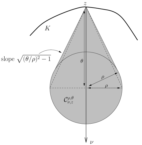
Figure 1. ${\mathcal{C}}_{\nu,z}^{\rho,\theta}$: interior cone at $z$ of parameters $\rho,\theta$ and axis $\nu.$

Figure 2. Illustration of the proof of Theorem 5.8.

Proof.

1. Restriction to a finite number of axes for the interior cones. We first observe that if $z\in\partial K$ and ${\mathcal{C}}_{\nu,z}^{\rho,\theta}\subset K$, then for all $\nu^{\prime}\in{\mathbb{S}}^{N-1}$ verifying $|\nu-\nu^{\prime}|\leq\rho/(2\theta)$, we have ${\mathcal{C}}_{\nu^{\prime},z}^{\rho/2,\theta}\subset K$. By compactness of ${\mathbb{S}}^{N-1}$, we can cover ${\mathbb{S}}^{N-1}$ with the traces on ${\mathbb{S}}^{N-1}$ of at most $p:={\beta(N)}/{(\rho/(2\theta))^{N-1}}$ balls of radius $\rho/(2\theta)$ centered at $\nu_{i}$, for some positive constant $\beta(N)$ and $1\leq i\leq p$. Therefore, for any $z\in\partial K$, there exists $1\leq i\leq p$ such that ${\mathcal{C}}_{\nu_{i},z}^{\rho/2,\theta}\subset K$.

2. Local study of points of the boundary with the same interior cone axis. We fix $1\leq i\leq p$ and set $A_{i}=\{z\in\partial K;\;{\mathcal{C}}_{\nu_{i},z}^{\rho/2,\theta}\subset K\}$. Up to a rotation of $K$, we can assume that $\nu_{i}=(0,\dots,0,-1)=:\nu$. Let us fix $z\in A_{i}$, that we write $z=(x,y)$ with $x\in{\mathbb{R}}^{N-1}$ and $y\in{\mathbb{R}}$. Let us set $V=B_{N-1}(x,\rho/4)\times\left(y-{\theta}/{2},y+{\theta}/{2}\right)$ and

$$D_{i}=\overline{V}\cap\underset{(x^{\prime},y^{\prime})\in A_{i}\cap\overline{V}}{\bigcup}{\mathcal{C}}_{\nu_{i},(x^{\prime},y^{\prime})}^{\rho/2,\theta}.$$

Then $A_{i}\cap V\subset\partial D_{i}\cap V$: indeed if $(x^{\prime},y^{\prime})\in A_{i}\cap V$, then $(x^{\prime},y^{\prime})\in D_{i}\cap V$, and $(x^{\prime},y^{\prime})$ can not lie in the interior of $D_{i}$, otherwise for $\lambda>0$ small enough, we would have $(x^{\prime},y^{\prime})-\lambda\nu\in D_{i}$, which would imply that $(x^{\prime},y^{\prime})$ lies in the interior of one of the cones forming $D_{i}$, and therefore in the interior of $K$, which is absurd since $(x^{\prime},y^{\prime})\in\partial K$.

3. The set $\partial D_{i}\cap V$ is a Lipschitz graph of constant $\sqrt{(2\theta/\rho)^{2}-1}.$ More precisely let us prove that $\partial D_{i}\cap V$ is equal to

$$G_{i} = \big{\{}(x^{\prime},y^{\prime}):x^{\prime}\in B_{N-1}(x,\rho/4)$$

$$\hskip 11.38092pt\text{and}\;y^{\prime}=\max\{y^{\prime\prime}:\;(x^{\prime},y^{\prime\prime})\in\partial{\mathcal{C}}\;\text{for one of the cones}\;{\mathcal{C}}\;\text{forming}\;D_{i}\}\big{\}}.$$

First of all, it is easy to show that $D_{i}$ is closed, and that the maximum in the definition of $G_{i}$ exists and is not equal to $y+\frac{\theta}{2}$; otherwise there would exist a cone ${\mathcal{C}}$ in $D_{i}$ such that $(x,y)\in{\rm int}({\mathcal{C}})\subset{\rm int}(K)$, which is absurd. The inclusion $G_{i}\subset\partial D_{i}\cap V$ follows from the same argument used for the inclusion $A_{i}\cap V\subset\partial D_{i}\cap V$ in Step 2. Conversely, let us fix $(x^{\prime},y^{\prime})\in\partial D_{i}\cap V$. Then $(x^{\prime},y^{\prime})\in D_{i}$ since $D_{i}$ is closed, so that $(x^{\prime},y^{\prime})$ is included in the trace on $V$ of one of the cones forming $D$, let us say $(x^{\prime},y^{\prime})\in{\mathcal{C}}$. But then $(x^{\prime},y^{\prime})$ can not belong to ${\rm int}({\mathcal{C}})$, otherwise we would have $(x^{\prime},y^{\prime})\in{\rm int}(D_{i})$, so we deduce that $(x^{\prime},y^{\prime})\in\partial{\mathcal{C}}\cap V$. Moreover if there exists $y^{\prime\prime}>y^{\prime}$ such that $(x^{\prime},y^{\prime\prime})\in\partial{\mathcal{C}}^{\prime}$ for some other of the cones ${\mathcal{C}}^{\prime}$ forming $D_{i}$, then we must have $(x^{\prime},y^{\prime})\in{\rm int}({\mathcal{C}}^{\prime})\cap V\subset{\rm int}(D_{i})$, which is absurd, and proves that $y^{\prime}$ is equal to the maximum in the definition of $G_{i}$, and that $\partial D_{i}\cap V\subset G_{i}$. Therefore $\partial D_{i}\cap V$ is a Lipschitz graph of constant $\mu=\sqrt{(2\theta/\rho)^{2}-1}$ as a supremum of graphs of cones of same parameters $\rho$ and $\theta$.

4. Estimate of the perimeter of $A_{i}$ in $V.$ It follows from Step 3 that $\partial D\cap V$ is ${\mathcal{H}}^{N-1}$ measurable with

$${\mathcal{H}}^{N-1}(\partial D\cap V)\leq{\mathcal{L}}^{N-1}(B_{N-1}(x,\rho/4))\,\sqrt{1+\mu^{2}},$$

hence

$${\mathcal{H}}^{N-1}(A_{i}\cap V)\leq\omega_{N-1}\left(\frac{\rho}{4}\right)^{N-1}\,\frac{2\theta}{\rho},$$

where $\omega_{j}$ denotes the volume of the unit ball of ${\mathbb{R}}^{j}$.

5. Covering of $A_{i}$ with balls of fixed radius. By Besicovitch’s covering theorem (see [12]), there exists a constant $\xi_{N}$ depending only on $N$ such that for any $\varepsilon>0$ and $R>0$, there exist numbers $\Gamma_{1},\dots,\Gamma_{\xi_{N}}$ and a finite family $(x_{kj})$ (for $1\leq k\leq\xi_{N}$ and $1\leq j\leq\Gamma_{k}$) of points of $A_{i}\cap\bar{B}(0,R)$ such that

$$\left\{\begin{aligned} &A_{i}\cap\bar{B}(0,R)\subset\bigcup_{k=1}^{\xi_{N}}\bigcup_{j=1}^{\Gamma_{k}}\bar{B}(x_{kj},\varepsilon),\\ &\text{for each}\;k,\text{the balls}\;\bar{B}(x_{kj},\varepsilon),\;1\leq j\leq\Gamma_{k},\,\text{are pairwise disjoint}.\end{aligned}\right.$$

The family $(x_{kj})_{j}$ is a priori only countable, but has to be finite by boundedness of $A_{i}$ and because the radius of covering balls is fixed. We now want to estimate $\sum_{k=1}^{\xi_{N}}\Gamma_{k}$. Let us therefore compute

$$\int_{K\cap\bar{B}(0,R+\varepsilon)}\sum_{k=1}^{\xi_{N}}\sum_{j=1}^{\Gamma_{k}}{11}_{\bar{B}(x_{kj},\varepsilon)}.$$

On the one hand, we have

$$\sum_{k=1}^{\xi_{N}}\int_{K\cap\bar{B}(0,R+\varepsilon)}\sum_{j=1}^{\Gamma_{k}}{11}_{\bar{B}(x_{kj},\varepsilon)}\leq\xi_{N}{\mathcal{L}}^{N}(K\cap\bar{B}(0,R+\varepsilon)),$$ (5.9)

because for each $k$, the balls $\bar{B}(x_{kj},\varepsilon)$ are pairwise disjoint. On the other hand, for each $k$ and $j$, the ball $\bar{B}(x_{kj},\varepsilon)$ contains a fixed portion of the cone ${\mathcal{C}}_{\nu_{i},x_{kj}}^{\rho/2,\theta}$, portion which is included in $K\cap\bar{B}(0,R+\varepsilon)$ by the interior cone property, since $x_{kj}\in A_{i}\cap\bar{B}(0,R)$. We call

$$\gamma:={\mathcal{L}}^{N}(\bar{B}(x_{kj},\varepsilon)\cap{\mathcal{C}}_{\nu_{i},x_{kj}}^{\rho/2,\theta})$$

the volume of this portion of cone, the computation of which is done in Step 7. Note that $\gamma$ is independent of $x_{kj}.$ Therefore

$$\int_{K\cap\bar{B}(0,R+\varepsilon)}\sum_{k=1}^{\xi_{N}}\sum_{j=1}^{\Gamma_{k}}{11}_{\bar{B}(x_{kj},\varepsilon)}=\sum_{k=1}^{\xi_{N}}\sum_{j=1}^{\Gamma_{k}}\int_{K\cap\bar{B}(0,R+\varepsilon)}{11}_{\bar{B}(x_{kj},\varepsilon)}\geq\sum_{k=1}^{\xi_{N}}\Gamma_{k}\gamma.$$ (5.10)

From (5.9) and (5.10), we deduce

$$\sum_{k=1}^{\xi_{N}}\Gamma_{k}\leq\frac{\xi_{N}}{\gamma}{\mathcal{L}}^{N}(K\cap\bar{B}(0,R+\varepsilon)).$$

Since $B((x,y),\varepsilon)\subset V=B_{N-1}(x,\rho/4)\times\left(y-{\theta}/{2},y+{\theta}/{2}\right),$ as soon as $\varepsilon<{\rm min}\{\rho/4,{\theta}/{2}\}=\rho/4$, we deduce from this that $A_{i}\cap\bar{B}(0,R)$ can be covered by $\sum_{k=1}^{\xi_{N}}\Gamma_{k}$ cylinders of the form of $V$ centered at points of $A_{i}\cap\bar{B}(0,R)$, so that, from (5.9),

$${\mathcal{H}}^{N-1}(A_{i}\cap\bar{B}(0,R)) \leq\sum_{k=1}^{\xi_{N}}\Gamma_{k}\,\omega_{N-1}\left(\frac{\rho}{4}\right)^{N-1}\,\frac{2\theta}{\rho}$$

$$\leq\frac{\xi_{N}}{\gamma}\,\omega_{N-1}\left(\frac{\rho}{4}\right)^{N-1}\,\frac{2\theta}{\rho}\,{\mathcal{L}}^{N}(K\cap B(0,R+\varepsilon)).$$

6. Sum for all axes. What we have done does not depend on the fixed direction axis $\nu_{i}$, and we know, thanks to Step 1 that $\partial K$ is the union of less than $p=\frac{\beta(N)}{(\rho/2\theta)^{N-1}}$ sets of the form $A_{i}$, so that we finally have

$${\mathcal{H}}^{N-1}(\partial K\cap B(0,R))\leq\frac{\beta(N)}{(\rho/2\theta)^{N-1}}\,\frac{\xi_{N}}{\gamma}\,{\omega_{N-1}\left(\frac{\rho}{4}\right)^{N-1}}\,\frac{2\theta}{\rho}\,{\mathcal{L}}^{N}(K\cap B(0,R+\varepsilon))$$

which gives (5.8).

7. Computation of the value of $\gamma.$ As soon as $\varepsilon\leq\sqrt{\theta^{2}-(\rho/2)^{2}}$ (the length of the longest segment included in $\partial{\mathcal{C}}_{\nu_{i},x_{kj}}^{\rho/2,\theta}$), then $\bar{B}(x_{kj},\varepsilon)$ contains at least the straight portion of ${\mathcal{C}}_{\nu_{i},x_{kj}}^{\rho/2,\theta}$ of length $l=\rho\mu\varepsilon/(2\theta)$, the volume of which equals

$$\frac{\omega_{N-1}}{N}\frac{l^{N}}{\mu^{N-1}}=\frac{\omega_{N-1}}{N}\mu\left(\frac{\rho}{2\theta}\varepsilon\right)^{N}.$$

This gives a lower bound for $\gamma$. Moreover, we obtain a more precise estimate for $\Lambda$ in (5.8): since $\rho<\theta$, we see that $\rho/4\leq\sqrt{\theta^{2}-(\rho/2)^{2}}$, so that sending $\varepsilon$ to $\rho/4$, we get

$${\mathcal{H}}^{N-1}(\partial K\cap\bar{B}(0,R))\leq 4^{N+1}N\beta(N)\xi_{N}\,\frac{1}{\rho}\frac{(\theta/\rho)^{2N}}{\sqrt{(2\theta/\rho)^{2}-1}}\;{\mathcal{L}}^{N}(K\cap B(0,\bar{B}+\rho/4)).$$

∎

5.4. Propagation of the interior cone property

We want to prove that the interior cone property is preserved for sets whose evolution is governed by the Eikonal equation (1.4). We assume:

(H7) The function $c(\cdot,t)$ is Lipschitz continuous with a constant independant of $t\in[0,T]$ and, for all $R>0,$ there exists an increasing modulus of continuity $\omega_{R}$ such that, for all $x\in B(0,R),$ $t,s\in[0,T],$ then

$$|c(x,t)-c(x,s)|\leq\omega_{R}(|t-s|).$$

Theorem 5.9.

Assume that $c$ satisfies (H1) and (H7) and that that $u_{0}$ satisfies (H6). Let $u$ be the unique uniformly continuous viscosity solution of (1.4). Then there exist $\rho>0$ and $\theta>0$ depending only on $K_{0}$, $N$, $\bar{c}$, $\underline{c}$ and $C$, such that $K(t)=\{x\in{\mathbb{R}}^{N};\;u(x,t)\geq 0\}$ has the interior cone property of parameters $\rho$ and $\theta$ for all $t\in[0,T]$. More precisely, let $r>0$ be such that $K_{0}$ has the interior ball property of radius $r>0$, then we can choose

$$\theta=\min\left\{\frac{\underline{c}^{2}}{6C\overline{c}},\underline{c}\,\omega_{R}^{-1}\left(\frac{\underline{c}}{4}\right),r\right\}\quad\text{and}\quad\rho=\frac{\underline{c}}{2\overline{c}}\theta$$

where $R>0$ is such that $K_{0}+\overline{c}T\bar{B}(0,1)\subset\bar{B}(0,R).$

Proof of Theorem 5.9..

1. Minimal time function. We first remark that the assumption that $c(x,t)\leavevmode\nobreak\ \geq\leavevmode\nobreak\ \underline{c}$ implies that $t\mapsto u(x,t)$ is nondecreasing for any $x\in{\mathbb{R}}^{N}$. Moreover, this assumption and the finite speed of propagation property imply that if $u(x,t)=0$, then $u(x,s)>0$ for any $s\in(t,T]$. Therefore, the minimal time function

$$v(x)=\min\{t\in[0,T];\;u(x,t)\geq 0\}$$

is defined at points $x\in K(T)$, and for any $t\in[0,T]$,

$$\{x\in{\mathbb{R}}^{N};\;u(x,t)\geq 0\}=\{x\in{\mathbb{R}}^{N};\;v(x)\leq t\},$$

$$\{x\in{\mathbb{R}}^{N};\;u(x,t)=0\}=\{x\in{\mathbb{R}}^{N};\;v(x)=t\}.$$

Moreover, $v$ is $1/\underline{c}$-Lipschitz in $K(T)$: let us fix $x$ and $y$ in $K(T)$ with $v(x)\leq v(y)$. The function

$$\overline{u}:(z,t)\mapsto\underset{|z^{\prime}-z|\leq\underline{c}|t-v(x)|}{\sup}u(z^{\prime},v(x))$$

is the unique uniformly continuous viscosity solution (see [3]) of

$$\left\{\begin{array}[]{cl}\overline{u}_{t}(z,t)=\underline{c}|D\overline{u}(z,t)|&\text{in}\;{\mathbb{R}}^{N}\times(v(x),T),\\ \overline{u}(\cdot,v(x))=u(\cdot,v(x))&\text{in}\;{\mathbb{R}}^{N}.\end{array}\right.$$

The comparison principle for continuous viscosity solutions implies that $\overline{u}\leq u$ in ${\mathbb{R}}^{N}\times[v(x),T]$. In particular

$$\overline{u}(y,\frac{1}{\underline{c}}|x-y|+v(x))\leq u(y,\frac{1}{\underline{c}}|x-y|+v(x)),$$

which implies by definition of $\overline{u}$ and $v$ that

$$0=u(x,v(x))\leq\overline{u}(y,\frac{1}{\underline{c}}|x-y|+v(x))\leq u(y,\frac{1}{\underline{c}}|x-y|+v(x)),$$

from which the Lipschitz property follows, since we deduce that

$$v(y)\leq\frac{1}{\underline{c}}|x-y|+v(x).$$

2. Interior cone property at time $\bar{t}\in[\mu,T]$ for some $\mu>0.$ To prove the claim of the theorem, we will use arguments from control theory. For this we need the velocity $c$ to be ${\mathcal{C}}^{1}$ in space, additionnal condition that we can assume without loss of generality by replacing $c$ by suitable space convolution $c_{\delta}$ of $c$. Then we get the result for $c_{\delta}$, and, letting $\delta\to 0^{+}$, obtain the desired result since the constants $\theta$ and $\rho$ do not depend on $\delta$.

It is well-known that, for each time $t$, the set $K(t)$ can be seen as the reachable set from $K_{0}$ for the controlled system

$$x^{\prime}(t)=c(x(t),t){a}(t)\;\text{for}\;t\in[0,T],$$ (5.11)

where the control ${a}$ takes its values in the unit closed ball. Let $x$ be an extremal trajectory, i.e. a trajectory verifying $x(T)\in\partial K(T)$. For such a trajectory, it is easy to see that $t\mapsto u(x(t),t)$ is non-decreasing, from which we infer that $x(t)\in\partial K(t)$ for any $t\in[0,T]$, that is to say, $v(x(t))=t$.

The Pontryagine maximum principle [10] implies the existence of an adjoint $p$ such that the following system is satisfied on $[0,T]$:

$$\left\{\begin{aligned} x^{\prime}(t)&=c(x(t),t)\frac{p(t)}{|p(t)|},\\ -p^{\prime}(t)&=Dc(x(t),t)|p(t)|.\end{aligned}\right.$$ (5.12)

From now on, we fix $0\leq\bar{t}\leq T.$ From (5.12) and the regularity of $c$ we infer that, if we set $M=3C\overline{c}$, then for any $s\in[0,\bar{t}]$,

$$|x^{\prime}(s)-x^{\prime}(\bar{t})|\leq M(\bar{t}-s)+\omega_{R}(\bar{t}-s),$$

where $R:=R_{0}+{\overline{c}}T$ is given by Lemma 5.3. By integration on $[t,\bar{t}],$ we deduce that, for any $t\in[0,\bar{t}]$,

$$|x(\bar{t})-x(t)-x^{\prime}(\bar{t})(\bar{t}-t)|\leq\frac{M}{2}(\bar{t}-t)^{2}+\omega_{R}(\bar{t}-t)(\bar{t}-t).$$ (5.13)

Let $x\in\partial K(\bar{t})$, and let $x(\cdot)$ be an extremal trajectory with $x(\bar{t})=x$. We are going to show that for any $t\in[0,\bar{t}]$, the ball $\bar{B}(t)$ of radius $r(t)$ centered at $x(\bar{t})-x^{\prime}(\bar{t})(\bar{t}-t)$ is contained in $K(\bar{t})$ for some $r(t)$ to determine, i.e. that we have for any $\xi\in\bar{B}(0,r(t))$,

$$v\left(x(\bar{t})-x^{\prime}(\bar{t})(\bar{t}-t)+\xi\right)\leq\bar{t}.$$

We therefore estimate, using the Lipschitz continuity of $v$ and (5.13),

$$\bar{t}-v\left(x(\bar{t})-x^{\prime}(\bar{t})(\bar{t}-t)+\xi\right)$$

$$\geq \bar{t}-v\left(x(\bar{t})-x^{\prime}(\bar{t})(\bar{t}-t)\right)-\frac{1}{\underline{c}}|\xi|$$

$$\geq \bar{t}-v(x(t))-\frac{1}{\underline{c}}\left(\frac{M}{2}(\bar{t}-t)^{2}+\omega_{R}(\bar{t}-t)(\bar{t}-t)\right)-\frac{1}{\underline{c}}r(t)$$

$$= \bar{t}-t-\frac{1}{\underline{c}}\left(\frac{M}{2}(\bar{t}-t)^{2}+\omega_{R}(\bar{t}-t)(\bar{t}-t)+r(t)\right).$$

Thus if we set $r(t)=\frac{\underline{c}}{2}(\bar{t}-t)$, the above quantity is nonnegative as soon as

$$\bar{t}-t\leq\frac{\underline{c}}{2M}\quad\text{and}\quad\omega_{R}(\bar{t}-t)\leq\frac{\underline{c}}{4}.$$

For this choice, it follows

$$\bar{B}(t) = \bar{B}\left(x(\bar{t})-x^{\prime}(\bar{t})(\bar{t}-t),r(t)\right)$$

$$= \left\{x(\bar{t})-\frac{x^{\prime}(\bar{t})}{|x^{\prime}(\bar{t})|}|x^{\prime}(\bar{t})|(\bar{t}-t)+\frac{\underline{c}}{2|x^{\prime}(\bar{t})|}|x^{\prime}(\bar{t})|(\bar{t}-t)\xi,\ \xi\in\bar{B}(0,1)\right\}$$

$$\subset K(\bar{t}).$$

Since $x(\bar{t})=x$ and $\underline{c}\leq|x^{\prime}(\bar{t})|\leq\overline{c}$, this proves the interior cone property at $x$ as soon as $\bar{t}\geq\mu=\min\left(\frac{\underline{c}}{2M},\omega_{R}^{-1}\left(\frac{\underline{c}}{4}\right)\right)$, of parameters

$$\rho_{1}=\frac{\underline{c}}{2\overline{c}}\,\theta_{1},\quad\text{with}\quad\theta_{1}=\min\left(\frac{\underline{c}^{2}}{2M},\underline{c}\omega_{R}^{-1}\left(\underline{c}/4\right)\right).$$

3. Interior cone property for small time $\bar{t}\in[0,\mu].$ With the previous notation, let $x\in\partial K(\bar{t})$ and $x(\cdot)$ be an extremal trajectory of (5.11) with $x(\bar{t})=x$. Let us recall that the regularity of $K_{0}$ implies that it has the interior ball property, i.e. there exists $r>0$ independent of $y\in\partial K_{0}$ such that

$$\bar{B}(y-\nu(y)r,r)\subset K_{0},$$

where $\nu(y)$ is the unit outer normal to $K_{0}$ at $y\in\partial K_{0}$. Note that, as a consequence, $K_{0}$ has the interior cone property at $x(0)$ of parameters $\rho=r/2$ and $\theta=r$ and $\nu(x(0))=p(0)/|p(0)|$. We see by the regularity of $K_{0}$ that $\nu(x(0))=p(0)/|p(0)|$, so that

$$\bar{B}(x(0)-\frac{p(0)}{|p(0)|}r,r)\subset K_{0}.$$ (5.14)

We will prove that, for $\bar{t}\leq\mu$, $K(\bar{t})$ has the interior cone property of parameters $\rho=r/2$ and $\theta=r$. Let $y\in{\mathcal{C}}_{\nu,x}^{r/2,r}$ with $\nu=-\frac{p(\bar{t})}{|p(\bar{t})|}$. We write $y$ as

$$y=x-\frac{p(\bar{t})}{|p(\bar{t})|}\lambda+\frac{1}{2}\lambda\xi,$$ (5.15)

where $0\leq\lambda\leq r$ and $|\xi|\leq 1$. Let $y(\cdot)$ be the solution of

$$\left\{\begin{aligned} y^{\prime}(t)&=c(y(t),t)\frac{p(t)}{|p(t)|}\quad\text{for}\;t\in[0,\bar{t}],\\ y(\bar{t})&=y,\end{aligned}\right.$$

where $p(\cdot)$ is the adjoint associated with $x(\cdot)$ by (5.12). It is enough to prove that $y(0)\in K_{0}$, since then $y=y(\bar{t})\in K(\bar{t})$. Because of (5.14), we only have to show that

$$\left|y(0)-\left(x(0)-\frac{p(0)}{|p(0)|}\lambda\right)\right|\leq\lambda.$$

Moreover, we remark that (5.15) implies that

$$\left|y(\bar{t})-\left(x(\bar{t})-\frac{p(\bar{t})}{|p(\bar{t})|}\lambda\right)\right|=|\frac{1}{2}\lambda\xi|\leq\frac{\lambda}{2}.$$

Let us therefore set

$$f(t)=|y(t)-x(t)+\lambda\frac{p(t)}{|p(t)|}|^{2},$$

so that $f(\bar{t})\leq\frac{\lambda^{2}}{4}$. It only remains to prove that $f(0)\leq\lambda^{2}$. But

$$f^{\prime}(t) = 2\left\langle y(t)-x(t),y^{\prime}(t)-x^{\prime}(t)\right\rangle+2\lambda\left\langle y^{\prime}(t)-x^{\prime}(t),\frac{p(t)}{|p(t)|}\right\rangle$$

$$\quad\quad\quad\quad\quad+2\lambda\left\langle y(t)-x(t),\frac{d}{dt}\frac{p(t)}{|p(t)|}\right\rangle$$

$$= 2\left\langle y(t)-x(t),\left(c(y(t),t)-c(x(t),t)\right)\frac{p(t)}{|p(t)|}\right\rangle$$

$$\quad\quad\quad\quad\quad+2\lambda\left\langle\left(c(y(t),t)-c(x(t),t)\right)\frac{p(t)}{|p(t)|},\frac{p(t)}{|p(t)|}\right\rangle$$

$$\quad\quad\quad\quad\quad+2\lambda\left\langle y(t)-x(t),\frac{p^{\prime}(t)}{|p(t)|}-\frac{p(t)\left\langle p(t),p^{\prime}(t)\right\rangle}{|p(t)|^{3}}\right\rangle$$

$$\geq -2C|y(t)-x(t)|^{2}-2\lambda C|y(t)-x(t)|-2\lambda|y(t)-x(t)|\left|\frac{p^{\prime}(t)}{|p(t)|}\right|$$

$$\quad\quad\quad\quad\quad-2\lambda|y(t)-x(t)|\left|\frac{p(t)\left\langle p(t),p^{\prime}(t)\right\rangle}{|p(t)|^{3}}\right|.$$

Thanks to (5.12), we know that

$$\left|\frac{p^{\prime}(t)}{|p(t)|}\right|\leq C\quad\text{and}\quad\left|\frac{p(t)\langle p(t),p^{\prime}(t)\rangle}{|p(t)|^{3}}\right|\leq C,$$

so that

$$f^{\prime}(t)\geq-2C|y(t)-x(t)|^{2}-6\lambda C|y(t)-x(t)|.$$

But if we set $g(t)=|y(t)-x(t)|^{2}$, then

$$g^{\prime}(t)=2\langle y(t)-x(t),y^{\prime}(t)-x^{\prime}(t)\rangle\geq-2C|y(t)-x(t)|^{2}=-2Cg(t),$$

which implies that for all $t\in[0,\bar{t}]$

$$g(t)e^{2Ct}\leq g(\bar{t})e^{2C\bar{t}},$$

that is to say thanks to (5.15)

$$|y(t)-x(t)|\leq|y-x|e^{C(\bar{t}-t)}\leq\frac{3\lambda}{2}e^{C\bar{t}}.$$

We therefore obtain

$$f^{\prime}(t)\geq-2C\left(\frac{3\lambda}{2}e^{C\bar{t}}\right)^{2}-6\lambda C\,\frac{3\lambda}{2}e^{C\bar{t}}=-\left(\frac{9}{2}Ce^{2C\bar{t}}+9Ce^{C\bar{t}}\right)\lambda^{2}.$$

If we set $k=\frac{9}{2}Ce^{2C\bar{t}}+9Ce^{C\bar{t}}$, we finally have

$$f(0)\leq f(\bar{t})+k\lambda^{2}\bar{t}\leq\frac{\lambda^{2}}{4}+k\lambda^{2}\bar{t}\leq\lambda^{2}$$

as soon as $k\bar{t}\leq\frac{3}{4}$. Thus if we set ${b}$ to be the unique solution of $\frac{9}{2}{b}e^{2{b}}+9{b}e^{{b}}=\frac{3}{4}$ (${b}>0$), we get that $f(0)\leq 0$ as soon as $\bar{t}\leq{b}/C$. If we assume that

$$\frac{b}{C}\geq\frac{\underline{c}}{2M}=\frac{\underline{c}}{6C\overline{c}},$$

which is always possible by reducing $\underline{c}$ or increasing $\overline{c}$, we see that $K(\bar{t})$ has the interior cone property of parameters $\rho_{2}=r/2$ and $\theta_{2}=r$ for all $0\leq\bar{t}\leq\mu$ (note that the parameters $\rho_{2},\theta_{2}$ depend only on $c$ and $K_{0}$).

4. End of the proof. We remark that

$$\frac{\rho_{1}}{\theta_{1}}=\frac{\underline{c}}{2\overline{c}}\leq\frac{1}{2}=\frac{\rho_{2}}{\theta_{2}},$$

whence we finally obtain that for any $\bar{t}\geq 0$, $K(\bar{t})$ has the interior cone property of parameters $\rho=\frac{\underline{c}}{2\overline{c}}\theta$ with $\theta=\min\{\theta_{1},\theta_{2}\}$. ∎

References

- [1] O. Alvarez, P. Cardaliaguet, and R. Monneau. Existence and uniqueness for dislocation dynamics with nonnegative velocity. Interfaces Free Bound., 7:415–434, 2005.
- [2] O. Alvarez, P. Hoch, Y. Le Bouar, and R. Monneau. Dislocation dynamics: short-time existence and uniqueness of the solution. Arch. Ration. Mech. Anal., 181(3):449–504, 2006.
- [3] G. Barles. Solutions de viscosité des équations de Hamilton-Jacobi. Springer-Verlag, Paris, 1994.
- [4] G. Barles, P. Cardaliaguet, O. Ley and R. Monneau. Global existence results and uniqueness for dislocation equations. To appear in SIAM J. Math. Anal.
- [5] G. Barles, P. Cardaliaguet, O. Ley and A. Monteillet. Existence of weak solutions for general nonlocal equations. Preprint.
- [6] G. Barles and O. Ley. Nonlocal first-order Hamilton-Jacobi equations modelling dislocations dynamics. Comm. Partial Differential Equations, 31(8):1191–1208, 2006.
- [7] G. Barles, H. M. Soner, and P. E. Souganidis. Front propagation and phase field theory. SIAM J. Control Optim., 31(2):439–469, 1993.
- [8] M. Bourgoing. Vicosity solutions of fully nonlinear second order parabolic equations with -time dependence and neumann boundary conditions. To appear in Discrete and Continuous Dynamical Systems.
- [9] M. Bourgoing. Vicosity solutions of fully nonlinear second order parabolic equations with -time dependence and neumann boundary conditions. existence and applications to the level-set approach. To appear in Discrete and Continuous Dynamical Systems.
- [10] F. H. Clarke. The maximum principle under minimal hypotheses, SIAM J. Control Optimization, 14(6):1078–1091, 1976.
- [11] M. G. Crandall and P.-L. Lions. Viscosity solutions of Hamilton-Jacobi equations. Trans. Amer. Math. Soc., 277(1):1–42, 1983.
- [12] Evans, L.C.; Gariepy, R.F., Measure theory and fine properties of functions, Studies in Advanced Mathematics, CRC Press, Boca Raton, FL, 1992.
- [13] Y. Giga, S. Goto, and H. Ishii. Global existence of weak solutions for interface equations coupled with diffusion equations. SIAM J. Math. Anal., 23(4):821–835, 1992.
- [14] H. Ishii. Hamilton-Jacobi equations with discontinuous Hamiltonians on arbitrary open sets. Bull. Fac. Sci. Eng. Chuo Univ., 28:33–77, 1985.
- [15] O. Ley. Lower-bound gradient estimates for first-order Hamilton-Jacobi equations and applications to the regularity of propagating fronts. Adv. Differential Equations, 6(5):547–576, 2001.
- [16] P.-L. Lions and B. Perthame. Remarks on Hamilton-Jacobi equations with measurable time-dependent Hamiltonians. Nonlinear Anal., 11(5):613–621, 1987.
- [17] A. Monteillet. Integral formulations of the geometric eikonal equation. Interfaces Free Bound., 9(2):253–283, 2007.
- [18] D. Nunziante. Uniqueness of viscosity solutions of fully nonlinear second order parabolic equations with discontinuous time-dependence. Differential Integral Equations, 3(1):77–91, 1990.
- [19] D. Nunziante. Existence and uniqueness of unbounded viscosity solutions of parabolic equations with discontinuous time-dependence. Nonlinear Anal., 18(11):1033–1062, 1992.
- [20] D. Rodney, Y. Le Bouar, and A. Finel. Phase field methods and dislocations. Acta Materialia, 51:17–30, 2003.
- [21] P. Soravia and P. E. Souganidis. Phase-field theory for FitzHugh-Nagumo-type systems. SIAM J. Math. Anal., 27(5):1341–1359, 1996.