S. N. Bose National Centre for Basic Sciences, Kolkata, sanjay1@bose.res.in
Lattice Fermion models Metal-insulator transitions and other electronic transitions Theories and models;localized states
Dimensional and temperature dependence of metal insulator transition in correlated and disordered systems
Abstract
We study the dimensional dependence of the interplay between correlation and disorder in two dimension at half filling using 2D disordered Hubbard model with deterministic disorder both at zero and finite temperatures. Inclusion of without disorder leads to a metallic phase at half filling below a certain critical value of . Above this critical value correlation favours antiferromagnetic phase. Since disorder leads to double occupancy over the lower energy site, the competition between Hubbard and disorder leads to the emergence of a metallic phase, which can be quantified by the calculation of Kubo conductivity, gap at half-filling , density of states, spin order parameter, Inverse participation ratio (IPR) and bandwidth. We have studied the effect of disorder on the system in a very novel way through a deterministic disorder which follows a Fibonacci sequence. Behaviour of different parameters show interesting features on going from a two to quasi one dimensional system.
pacs:
71.10.Fdpacs:
71.30.+hpacs:
71.23.An1 Introduction
Kravchenko [1] in a series of experiments on very weakly disordered 2D semiconductors (Si MOSFETS) at very low filling, in the absence of magnetic field showed that it is possible for a 2D system to undergo Metal Insulator transition. Recently Punnoose and Finkelstein have shown that it is possible to identify a Quantum Critical point separating a metallic phase stabilized by electronic interactions from the insulating phase where disorder prevails over electronic interactions in certain systems [2].
Recently the Mott Insulator has been realised for fermionic atoms in an optical lattice in 3 dimensions[3] whereas most of the previous results were for Bosonic atoms. Further the experimental realisation of Anderson insulators for Bose gas has been realised[4] by disordering the optical lattice site potentials. It is possible to disorder the lattice in a rather controlled manner on optical lattices. This has facilitated the controlled experimental study of the phase diagram arising due to the competition of strong correlations and disorder in these systems, causing us to revisit this topic.
The present work emphasizes on the dimensional dependence of the interplay between electronic correlation and deterministic disorder (and the consequential reflection in metal insulator transition(MIT)) as one goes from a two dimensional system to a quasi one dimensional system. Also the important aspect of the role of temperature in this whole scenario has been duly addressed.
A Hartree Fock mean field treatment of the non-disordered Hubbard Hamiltonian [5] shows Paramagnetic to Antiferromagnetic transition at = 2.1.e The disordered Hubbard hamiltonian was shown to have persistent currents [6], Milovanović et al [7] investigated it numerically and Bhatt et al [8] studied local moment formation. Dobrosavljević and co-workers [9] use generalized DMFT method to report the interesting fact that increasing disorder from a clean Mott insulator results in the closing of the Mott gap and the stabilization of a metallic phase.
The possibility that a metallic phase may exist in 2D due to the interplay of strong correlations and random disorder for the half filled disordered Hubbard Model has been suggested [10].
We solve the problem numerically using Unrestricted Hartree Fock(UHF) technique. The UHF method works remarkably well even in 1D at half-filling and is in excellent agreement with results obtained from real space renormalization method [11]. In 2D at half filling the UHF method gives result in close proximity with that of quantum monte carlo method [5]. However, one should mention here that the correlated Kondo like processes that lead to large effective-mass renormalization in the vicinity of the Mott transition can only be captured by a method like DMFT and not by the present method [12]. The importance of inelastic scattering processes for calculating the conductivity was shown by a DMFT calculation by Aguiar et. al [13]. We choose a deterministic binary disorder(that follows a Fibonacci sequence), motivated largely by optical lattice realisations. Deterministic disorder has been one of the forefront areas of research in condensed matter physics for the past two and a half decades both in experiments [14] and theory [15]. Theoretical studies of the quasi-periodic systems have shown that in the non-interacting limit the wave function shows a power law localization both in one [16] and two [17] dimensions. Very recent experiment in 1D quasi-periodic optical lattice [18] where the system was described by Aubry-Andre Hamiltonian has shown exponentially localized states (Anderson localization) in the large disorder limit. A theoretical explanation has been published recently [19] using a Fibonacci sequence in 1D. We benchmark our results and trends against old results obtained with random disorder. Zero and finite temperature calculations have been carried out for different values of the disorder strength. The impurity concentration remained almost constant as we reduced the dimension, which is an artifact of the Fibonacci sequence. We have taken a lattice which is fairly large to rule out finite size effects.
The system, though insulating in the regime, undergoes a depletion of the charge gap at half filling as the disorder is increased, till it reaches a stage where the lower energy sites would be doubly occupied in spite of the large value of . A narrow metallic regime emerges while going from the Neel state to the state with a distribution of doubly-occupied and unoccupied sites. The low temperature metallic phase gives way to an insulating phase upon heating. It has residual spin order(very low value) and is thus not a perfect paramagnet. One of our objectives in the present work is to investigate the evolution of the interplay between disorder and interactions and relatively whose effect gets more dominant as one reduces the dimension. The effect of next nearest neighbour hopping makes the delocalized phase more robust.
2 Disordered Hubbard Hamiltonian
The disordered 2D t-t’ Hubbard Hamiltonian considered by us is as follows:
| (1) |
| (2) |
| (3) |
Here and are nearest and next nearest neighbour hopping terms, is the on site Hubbard interaction, is the site potential at i-th site, while , , , are creation, annihilation operators for the electron of spin , and the number operators for up and down spins respectively at site .
3 Deterministic Disorder
Deterministic disorder is neither periodic nor fully random and have long range correlations(correlated disorder). The site potential is deterministically disordered. It follows a Fibonacci sequence which is generated as and , where and are the two different sites. In our case site has a higher site potential than site (, , being the disorder strength). A typical Fibonacci chain in a particular generation looks like: . We have used the Fibonacci sequence and generalised the idea of quasi-periodicity in one dimensions to two dimension by essentially wrapping up the one dimensional Fibonacci sequence over the two dimensional square lattice. Moreover the number of lattice sites need not be a Fibonacci number. In our case the lattice sites picks up the first entries of the sequence from the left, thus allocating the site potentials. This sort of disorder can also be referred to as correlated disorder.
| size | A | B | |
|---|---|---|---|
| 989 | 611 | 1.608 | |
| 346 | 214 | 1.616 | |
| 247 | 153 | 1.614 | |
| 148 | 92 | 1.608 |
4 Discussion of Numerical Method
We solve the Hartree Fock decoupled Hamiltonian with an initial guess(seed) of and , and solve it self-consistently till the solutions of and converge to a difference of less than for every site. We settled up with that initial seed which minimises the ground state energy. This strict convergence criterion has been employed to ensure that we stay away from local minimas while exploring the energy landscape. This is extremely important as we approach the disorder induced localized phase using a variational approach like Hartree Fock to treat interactions as our only guiding principle in choosing the ground state configuration is energetics. In the low and medium disorder regime if we start from the Neel order state as the starting seed, we get the desired convergence very quickly, while in the high disorder regime near the MIT, we have found the desired results starting with a near paramagnetic configuration as the initial seed(PM seed).
4.1 Unrestricted Hartree Fock
In UHF theory the Hubbard interaction term is decoupled keeping in the site dependence and thus one obtains modified site potentials for up and down spins which reads as:
| (4) |
This gives us the following Hamiltonian which is decoupled into up and down spin parts:
| (5) |
Where are now defined by eq. (4).
5 Quantities calculated
Once the energy spectrum is obtained the energy gap at half-filling is calculated by the difference between the energy level at half-filling and the one just above it. The expression reads as:
| (6) |
where is the number of sites in the 2D lattice. The ground state energy is calculated by summing up the single particle energy states for both spin species up to the Fermi level corresponding to the desired filling. The Fermi level at half filling is calculated as the mean of the highest filled state and the lowest unoccupied one to ensure that the system remains half filled. All finite temperature calculations are performed with respect to this Fermi energy with the appropriate Fermi distribution factors. If and are converged values of of the occupation numbers of up and down spins respectively at the i-th site, then the spin order is defined as:
| (7) |
For disordered non interacting systems, the Kubo formula, at any temperature is given by:
| (8) |
with , being the lattice spacing, and = Fermi function with energy . The are matrix elements of the current operator , between exact single particle eigenstates , , etc, and , are the corresponding eigenvalues. In this paper, conductivity/conductance is expressed in units of .
We calculate the ‘average’ conductivity over 3-4 small frequency intervals ( = , n = 1,2,3,4), and then differentiate the integrated conductivity to get at , n = 1,2,3. These three values are then extrapolated to to get . For the sake of simplicity, and keeping all other consistency checks in mind [20], we have taken the value of as the actual value of .
The average of over the interval is
| (9) |
is set to be sufficiently larger than the average spacing between energy levels, given by , where is the full bandwidth for the interacting 2D disordered Hubbard Model that we are considering and is simply calculated as , where and refer to the topmost and lowermost eigenvalues. For , .
In the discussion below, all length scales are normalized by the lattice parameter , and we use dimensionless energy parameters , and , scaled by the hopping amplitude .
IPR which gives the measure of how many sites are participating in a
particular eigenfunction is defined as following [21]:
| (10) |
where corresponds to the site index, is the nth eigenvalue. The cited ref calculated IPR for a non interacting system with Fibonacci modulated site potential. It is clearly visible from the above expression that larger value of IPR corresponds to localized electronic states whereas small value of IPR indicates an extended state. In our case the topmost eigenfunction near the Fermi level was considered for this purpose.
6 Numerical Results
We have calculated the gap at half filling, charge and spin order, bandwidth, IPR and the of the 2D disordered Hubbard model at half filling as we vary the , Disorder potential and also reduce the dimensionality along the y direction. We study the problem for intermediate disorder strength () where the underlying Neel magnetic ordering(due to ) is not killed and is predominantly present, for a lattice. We have shown here our calculations for system sizes and . We have tabulated the number of and sites and the ratio for the different sizes which is given in table 1
|
|
|
|
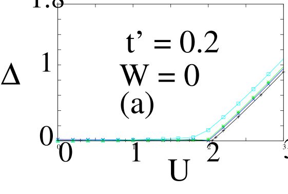
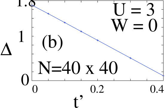
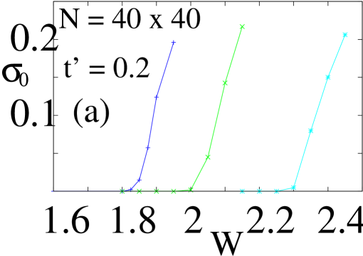
In Fig. 1a we study effect of size reduction along y axis. We show that for , is zero till a critical , above which it becomes non-zero and matches well with Hirsch’s result[5]. is unchanged all the way down to below which starts decreasing slowly at first, and below , it shows a steep fall, as the quasi 1D effect sets in and electronic motion gets constrained. In Fig. 1b decreases almost linearly as we increase , in the regime( ), as kills the Neel ordering due to .
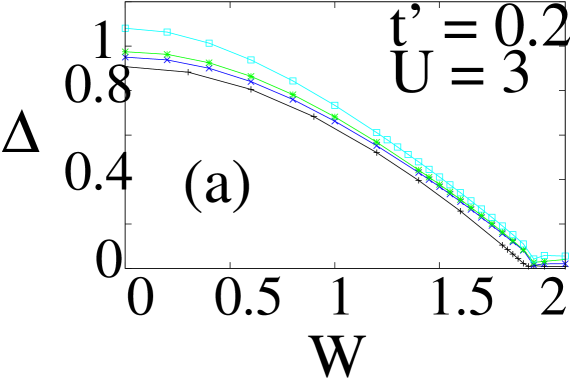
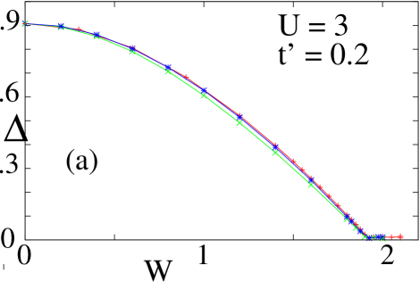
Fig. 2a shows the plot of the gap (as we reduce ) for against disorder strength for , which renders the undisordered phase antiferromagnetic. The disorder reduces the gap as now the electrons of both spin species will try to avoid the site with higher energy, thereby allowing some double occupancies on the lower energy site. The gap decreases rather slowly for low values of and finally falls sharply at a certain , for a fixed system size.
We find that for a fixed disorder, though increases as we reduce , the rate of fall in increases with increase in disorder as we reduce , highlighting that effect of disorder is more pronounced than the effect of Hubbard as one reduces . We will see the effect of this in our Kubo conductivity results.
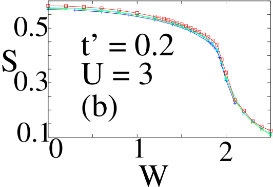
The corresponding spin order plot also follows a similar trend (Fig. 2b). However the reduction in this case is more gradual than the gap at half filling. This is because the system prefers to retain the antiferromagnetic configuration to gain maximum kinetic energy due to hopping, till a critical value of upto which is effective, and beyond which the spin order reduces very rapidly. We find this critical , at which point the Hubbard gap roughly diminishes from first to second place of decimal. The reduction in magnetic ordering is much slower than the gap at half filling, and there is significant residual magnetic ordering() when has already gone to zero.
|
|
|
|
|
|
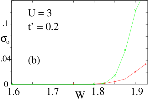
Fig. 3a shows the plot of the dc conductivity() against disorder strength at = 0 for = 3,3.2 and 3.4, which is well in the antiferromagnetic regime even for = 0.2. Due to interplay between correlation and disorder, increases from zero at a critical value of , whose value increases with . Thus it takes higher values of disorder to form doubly occupied sites as one increases at half filling. This plot cannot be extrapolated indefinitely on the lower side as has to be greater than .
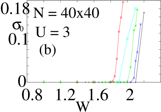
Fig. 3b shows the plot of Kubo conductivity at zero temperature as we change for the disordered problem. It is found that as we increase from zero it takes a lower value of disorder to first generate a non zero value of the Kubo conductivity and then render the system metallic.
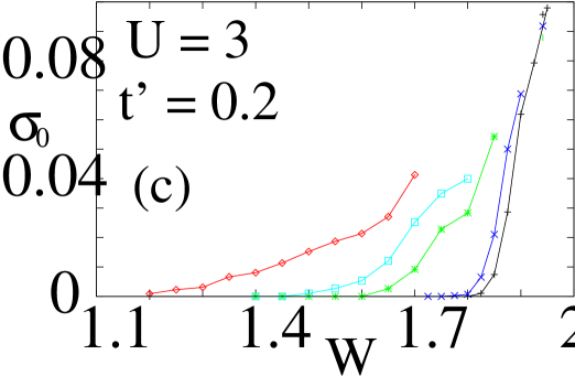
Fig. 3c shows the plot of the against as we reduce the system size along y direction, thus going over to a quasi-1D system. We need lower disorder value to annul the effect of , as we lower the dimensionality again highlighting the fact that the effect of disorder, for a fixed value of becomes more robust as we decrease the dimensionality from 2D to quasi 1D. The faster rate of depletion of the Hubbard gap as we reduce the dimensionality as seen in Fig. 2a, is thus connected to the curves for different in this way.
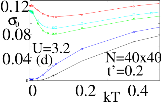
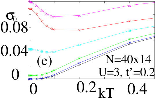
Fig. 3d show the plots of against temperature for and shows an insulator to metal transition with increasing at low temperatures. Our calculation shows a finite conductivity at zero temperature, which is consistent with experimental results. The region corresponds to the diffusive sector while for we are in the ballistic regime. corresponds to the value of for which at = 0 becomes non-zero and slowly starts to increase, while at the system becomes a metal as the Hubbard gap is completely killed by the disorder. In between there is a narrow range of within which starts increasing from zero, but the system is still however not a metal. Further increasing , we enter a metallic regime where the rate of fall in conductivity with temperature decreases. This indicates that it is a highly disordered metallic phase (dirty metal). The ground state of the highly disordered insulator is extremely difficult to obtain within Hartree Fock, which takes a very long time to converge to the required precision. Even when it does, there is a possibility of the system getting stuck in one of the many local minimas and not being able to access the true ground state. We therefore venture upto the point where there are no convergence problems(system is metallic).
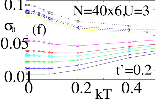
Though the effect of becomes stronger, with the Hubbard gap becoming larger as we decrease the dimensionality of the system, it is clear that disorder effect surpasses the effect of as one lowers the dimension as evident from Fig. 3(d,e,f). Fig. 3d,e,f shows the finite temperature plots of for different parametric values of for = 40, 14 and 6 respectively. We again observe the general behaviour that the dc conductivity of an insulator/metal rises/falls with increasing temperature in the low temperature regime. However the onset of the metallic phase occurs for lower values of as we reduce the dimensionality.
We see that as we heat the system, the system goes from a low temperature metallic phase to a high temperature insulator phase. This effect is further seen to go away as we reduce the dimensionality.
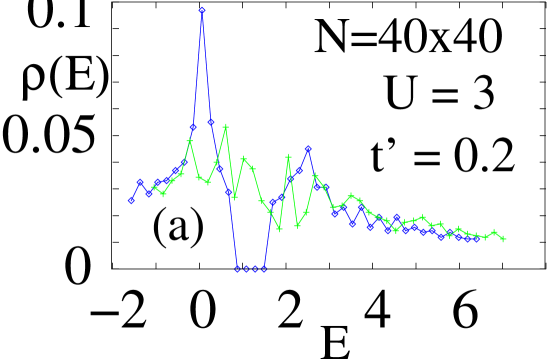
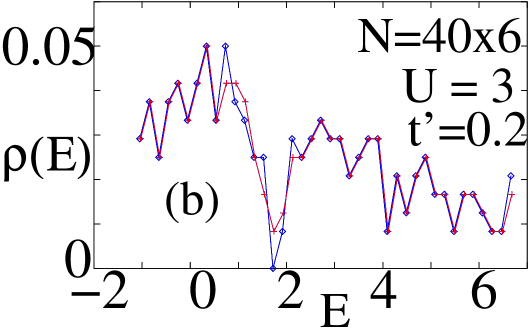
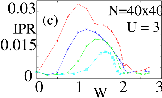
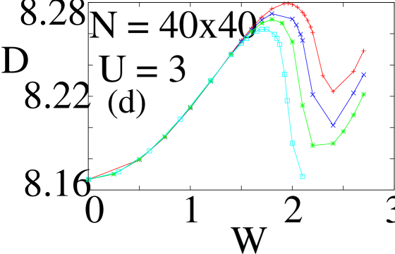
Fig. 4a,b shows the plot of the density of states(DOS) for a fixed value of = 3 for = 40 and 6 respectively, highlighting how disorder closes the gap when we reach . However the gap closes for lower value of as we decrease again emphasising the increased effectiveness of disorder as we reduce the dimensionality. We compare our result with the work done in the first reference of [9]. We observe from their LDOS plot that the MIT for the random disordered 2D Hubbard model occurs roughly at for . In our work for the 2D (for t’=0.2), deterministically disordered Hubbard model the MIT occurs at for (Fig. 4a). Fig. 4c,d shows the IPR and the bandwidth of the system for a fixed value of , as we increase the disorder strength. Fig. 4d clearly shows that for the interacting case the effect of disorder on band-width is quite non-monotonic and non-trivial. The bandwidth increases for very weak(low) disorder, then it stops growing and surprisingly starts decreasing with increasing disorder. This is the regime where the states at the Fermi energy have already become delocalized as can be seen from Fig. 4c(the IPR curve also behaves non-monotonically). In this regime more and more states are introduced in the gap region. Since total number of levels are fixed, the bandwidth decreases.
The localization in the Hartree Fock single particle excitations for , as reflected in the IPR peak below is rapidly eroded as we increase . This is seen in the rapidly falling peak structure in the IPR curve as we increase . Thus with increasing , there is a subtle transition in the nature of the wave-functions itself(localized to delocalized) as the metallic phase sets in.
|
|
|
|
Fig 5(a) represents the plot of gap at half filling against disorder, for three different realizations of the Fibonacci sequence. One can see from these plots that the results remain almost invariant as we change the realization. The results shown here are for = 3 and = 0.2 for a system.
Fig 5(b) shows our results of the dc conductivity at zero temperature as a function of disorder, in the range where the dc conductivity just starts to pick up from zero. We have shown the results for 2 system sizes, namely and . It is clearly observed that the critical value of disorder where the dc conductivity picks up from zero is almost the same. This shows that the finite size effects are already quite small by the time we reach system size.
|
|
We believe that our simulation results provides useful and direct insight into the competition between correlations and disorder, which has been introduced in a simplified(deterministic) manner and is capable of capturing all the subtleties involved. It gives a good estimate of the Kubo conductivity as one goes from 2D to quasi 1D systems in presence of disorder and correlation and indicates the emergence of a metallic phase. As we tune the disorder to a very high value, the system becomes a metallic glass(highly disordered metal).
Acknowledgements.
Sanjay Gupta thanks Shreekantha Sil for some valuable suggestion. Tribikram thanks Saptarshi Mandal for providing additional computational facility while on a visit to IMSc and Sanjeev Kumar for useful discussions.References
- [1] Elihu Abrahams, S. V. Kravechenko and M. P. Sarachik, Rev. Mod. Phys. 73, 251(2001)
- [2] A. Punnoose and A. M. Finkelstein, Science 310, 289 (2005)
- [3] Robert Jordens ,Nature 455, 204-207(2008); U. Schneider , Science 322,1520-1525(2008)
- [4] B. Damski , Physical Review Letter 91,080403(2003)
- [5] H. Q. Lin and J. E. Hirsch, Phys. Rev. B 35, 3359(1987)
- [6] G. Bouzerar, D. Poilblanc and G. Montambaux, Phys. Rev. B 49, 8258 (1994)
- [7] M. Milovanović, S.Sachdev, and R. N. Bhatt, Phys. Rev. Lett. 63, 82
- [8] Bhatt, R. N. and D. S. Fisher, Phys. Rev. Lett. 68, 3072
- [9] M. C. .O. Aguiar, V. Dobrosavljević, E. Abrahams, G. Kotliar, Phys. Rev. Lett. 102, 156402 (2009), E. C. Andrade, E. Miranda, V. Dobrosavljević, Phys. Rev. Lett. 102, 206403 (2009)
- [10] Dariyush Heidarian and Nandini Trivedi, Phys. Rev. Lett., 93, 126401
- [11] Sanjay Gupta, Shreekantha Sil and Bibhas Bhattacharyya, Phys. Rev. B 63, 125113 (2001).
- [12] M. Potthoff, W. Nolting, Physica B 259-261 760-761 (1999), P. Lederer and M. J. Rozenberg, EuroPhys. Lett. 81 67002 (2008)
- [13] M. C. O. Aguiar, E. Miranda, V. Dobrosavljevic, E. Abrahams and G. Kotliar, EuroPhysics Letters, 67(2), 226 (2004)
- [14] R. Merlin, K. Bajema, R. Clarke, F. Y. Juang and P. K. Bhattacharya, Phys. Rev. Lett 55, 1768(1985), J. Delahaye, T. Schaub, C. Berger and Y. Calvayrac, Phys. Rev. B 67, 214201 (2003),
- [15] Sanjay Gupta, Shreekantha Sil, Bibhas Bhattacharyya, Physica B. 355, 299 (2005), P. E. de Brito, E. S. Rodrigues, and H. N. Nazareno, Phys. Rev. B 73, 014301 (2006); P. W. Mauriz, E. L. Albuquerque, and M. S. Vasconcelos, Phys. Rev. B 63, 184203 (2001); M. S. Vasconcelos and E. L. Albuquerque, Phys. Rev. B 59, 11128 (1999)
- [16] Mahito Kohomoto and J. R. Banavar, Phys. Rev. B 34, 563(1986), B. Sutherland, Phys. Rev. B 39, 5834(1989)
- [17] B. Sutherland, Phys. Rev. B 34, 3904(1986)
- [18] G. Roati,C. D’Errico,L. Fllani,M. Fattori, C. Fort, M. Zaccanti, G. Modugno, M. Modugno, M. Inguscio, Nature 453, 895(2008)
- [19] M. Modugno, New Journal of Physics, 11, 033023(2009)
- [20] Sanjeev Kumar and Pinaki Majumdar, Europhys. Lett 65, 75 (2004)
- [21] F.Dominiguez-Adame, Physica B 307, 247-250(2001).