Dynamics of delay-coupled excitable neural systems

Abstract

We study the nonlinear dynamics of two delay-coupled neural systems each modelled by excitable dynamics of FitzHugh-Nagumo type and demonstrate that bistability between the stable fixed point and limit cycle oscillations occurs for sufficiently large delay times $\tau$ and coupling strength $C$. As the mechanism for these delay-induced oscillations we identify a saddle-node bifurcation of limit cycles.

I Introduction

The brain may be conceived as a dynamic network of coupled neurons HAK06 ; WIL99 ; GER02 . These neurons are excitable units which can emit spikes or bursts of electrical signals. In order to describe the complicated interaction between billions of neurons in large neural networks, the neurons are often lumped into highly connected sub-networks or synchronized sub-ensembles. Such neural populations are usually spatially localized and contain both excitatory and inhibitory neurons WIL72 .

The simplest model to display features of neural interaction consists of two coupled neural systems. Starting from this simplest network motif, larger networks can be built, and their effects may be studied. For example, starting from two interconnected reticular thalamic neurons with oscillatory behavior, it was shown in DES94 how more complex dynamics emerges in ring networks with nearest neighbors and fully reciprocal connectivity, or in networks organized in a two-dimensional array with proximal connectivity and “dense proximal” coupling in which every neuron connects to all other neurons within some radius. In another example ZHO06c , a neural population was itself modeled as a small sub-network of excitable elements, to study hierarchically clustered organization of excitable elements in a network of networks.

Most studies represent a population as an effective oscillatory element that is then coupled with other populations to study synchronization and network effects ROS04a ; POP05 ; GAS07b . In these studies, the basis for the emergence of complex network dynamics is the oscillatory behavior of neural elements, in spite of the fact that individual neural systems are usually in a stable steady state exhibiting excitable dynamics when perturbed. A reason is that self-sustained oscillatory behavior in the individual element is required to define synchronization of subsystems ROS01a . One way to resolve this is to add weak Gaussian white noise to each individual element to generate sparse Poisson-like irregular spiking patterns, as seen in real neurons ZHO06c ; HAU06 ; HOE07 .

In this report, we introduce a time-delayed coupling into the model of two excitable populations and demonstrate that the coupling-delay can induce sustained oscillations between the two subsystems. We find a regime of bistability between the stable fixed point and limit cycle oscillations for sufficiently large delay times $\tau$ and coupling strength $C$. As the mechanism for these delay-induced oscillations we identify a saddle-node bifurcation of limit cycles.

This result suggests the use of a compound system of two time-delayed coupled excitable elements as a minimal network motif to investigate oscillatory behavior in more complex networks.

II Model

We examine the delayed linear symmetric coupling of two identical neural populations. Each population is represented by a simplified FitzHugh-Nagumo (FHN) system FIT61 ; NAG62 , which is widely used as a paradigmatic model of excitable systems LIN04 .

The dynamical equations are given by:

$$\epsilon\dot{x_{1}} = x_{1}-\frac{x_{1}^{3}}{3}-y_{1}+C[x_{2}(t-\tau)-x_{1}(t)]$$

$$\dot{y_{1}} = x_{1}+a$$

$$\epsilon\dot{x_{2}} = x_{2}-\frac{x_{2}^{3}}{3}-y_{2}+C[x_{1}(t-\tau)-x_{2}(t)]$$

$$\dot{y_{2}} = x_{2}+a$$ (1)

where the two subsystems ($x_{1},y_{1}$) and ($x_{2},y_{2}$) correspond to two neuron populations. The value of the excitability parameter $a$ determines whether the subsystem is excitable ($a>1$) or exhibits self-sustained periodic firing ($a<1$). This is because at $a\!=\!1$ the uncoupled systems exhibit a Hopf bifurcation, and the fixed point becomes an unstable focus for $a\!<\!1$. $\epsilon$ is the timescale parameter that, if chosen to be much smaller than unity, results in fast activator variables $x_{1},x_{2}$, and slow inhibitor variables $y_{1},y_{2}$. Unless otherwise noted, we shall choose $\epsilon=0.01$ and $a\!=\!1.3$ for numerical simulations and thus restrict our analysis to parameter values where each of the two subsystems exhibits excitability with a stable fixed point.

The interaction between the two neural populations is modelled as diffusive, i. e., the coupling vanishes if the variables $x_{i}$ are identical. The coupling strength $C$ is taken to be symmetric for simplicity. Further, we assume a finite signal propagation speed between distant neural populations. This is incorporated using the delay time $\tau$. Note that the coupling term has the form of a classical diffusion term, but has lost its diffusive character through the introduction of a propagation delay $\tau$. More general delayed couplings are studied in BUR03 .

Before we analyse Eq. (II), let us briefly give a biophysical interpretation of the hitherto abstract nature of the dynamical variables $x_{i}$ and $y_{i}$. This is needed to relate our results to other work on population dynamics in neural networks, in particular to studies dealing with spiking rates and time delays PIN01 ; COO03 ; HUT03 ; HUT04 . These studies consider neural fields WIL73 ; AMA77 , that is, they extend over one or more spatial dimensions. While neural field models adopt the continuum limit of a network, we consider the minimal network motif, i. e., two discrete subsystems, but in both cases the biophysical reason to include delay is the same.

The generic biophysical interpretation of the FHN model is based on a single point-like neuron and was originally not derived from features of a neural population. The variable $x$ models fast changes of the electrical potential across the membrane (spikes), and $y$ is related to the gating mechanism of membrane channels FIT61 ; NAG62 . On the contrary, a neural population is generically described by a time coarse-grained mean-field model, in which the dynamical variables represent averaged spiking rates WIL72 . Notwithstanding, spiking rates in neural populations can exhibit both steady state values and relaxation oscillations. Both states are described by the FHN mechanism with $a\!>\!1$ and $a\!<\!1$, respectively, which justifies the FHN model for “point-like” populations. To avoid confusion about spikes vs. spiking rates, a model of uncoupled subsystems as defined by Eq. (II) with $C=0$ is sometimes referred to as the Bonhoeffer-van der Pol model POL26 ; POL29 ; BON48 , for example in Ref. ROS04 .

III Linear Stability Analysis

The unique fixed point of the system is symmetric and is given by ${\bf x}^{*}\equiv(x_{1}^{*},y_{1}^{*},x_{2}^{*},y_{2}^{*})$, where $x_{i}^{*}\!=\!-\!a$, $y_{i}^{*}\!=\!a^{3}/3\!-\!a$.

Denoting for convenience ${\bf x}(t\!-\!\tau)\equiv\tilde{\bf x}$, we can re-write system Eq. (II) as:

$$\left(\begin{array}[]{c}\dot{x_{1}}\\ \dot{y_{1}}\\ \dot{x_{2}}\\ \dot{y_{2}}\end{array}\right)=\left(\begin{array}[]{c}f_{1}(\bf{x})\\ f_{2}(\bf{x})\\ f_{3}(\bf{x})\\ f_{4}(\bf{x})\end{array}\right)+\left(\begin{array}[]{c}g_{1}(\bf{\tilde{x}})\\ g_{2}(\bf{\tilde{x}})\\ g_{3}(\bf{\tilde{x}})\\ g_{4}(\bf{\tilde{x}})\end{array}\right)$$ (14)

This system can be linearized around the fixed point $\bf{x}^{*}$ by setting ${\bf x}(t)=\bf{x}^{*}+\delta\bf{x}(t)$:

$$\delta\dot{\bf{x}}=\bf{J}_{f}^{*}\delta\bf{x}+\bf{\tilde{J}}_{g}^{*}\delta\tilde{\bf{x}}$$ (15)

with the Jacobian matrices $\bf{J}_{f}^{*}$ and $\bf{\tilde{J}}_{g}^{*}$. The explicit form is

$$\delta\dot{\bf{x}}=\frac{1}{\epsilon}\left(\begin{array}[]{cccc}\xi&-1&0&0\\ \epsilon&0&0&0\\ 0&0&\xi&-1\\ 0&0&\epsilon&0\end{array}\right)\delta\bf{x}+\frac{1}{\epsilon}\left(\begin{array}[]{cccc}0&0&C&0\\ 0&0&0&0\\ C&0&0&0\\ 0&0&0&0\end{array}\right)\delta\tilde{\bf{x}}$$ (24)

where $\xi=1-a^{2}-C$. The ansatz

$$\delta\bf{x}(t)=e^{\lambda t}\bf{u}$$ (25)

where $\bf{u}$ is an eigenvector of $\bf{J}_{f}^{*}$ implies

$$\delta\bf{\tilde{x}}=e^{\lambda t}e^{-\lambda\tau}\bf{u}$$ (26)

This leads to the characteristic equation

$$(1-\xi\lambda+\epsilon\lambda^{2})^{2}-(\lambda Ce^{-\lambda\tau})^{2}=0,$$ (27)

which can be factorized giving

$$1-\xi\lambda+\epsilon\lambda^{2}=\pm\lambda Ce^{-\lambda\tau}$$ (28)

This transcendental equation has infinitely many complex solutions $\lambda$. Fig. 1 shows the real parts of $\lambda$ for various values of $C$.

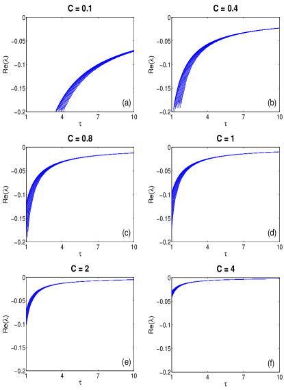
Figure 1: Real parts Re($\lambda$) of the eigenvalues of the fixed point vs. time delay $\tau$ for $\epsilon=0.01$, $a=1.3$, and (a) C=0.1, (b) C=0.4, (c) C=0.8, (d) C=1, (e) C=2, (f) C=4.

As can be seen in Fig. 1 the real parts of all eigenvalues are negative throughout, i. e., the fixed point of the coupled system remains stable for all $C$. This can be shown analytically for $a>1$ by demonstrating that no delay-induced Hopf bifurcation can occur. Substituting the ansatz $\lambda=i\omega$ into Eq. (28) and separating into real and imaginary parts yields for the imaginary part

$$\xi=\pm Ccos(\omega\tau)$$ (29)

This equation has no solution for $a>1$ since $|\xi|=a^{2}-1+C>C$, which proves that a Hopf bifurcation cannot occur.

IV Delay-induced oscillations

The cooperative dynamics of delay-induced oscillations in excitable systems is inherently different from those of noise-induced oscillations. The introduction of noise terms induces sustained oscillations in each individual subsystem by continuously kicking these subsystems out of their respective rest states. Coupling then produces synchronisation effects between these individual oscillators HAU06 ; HOE07 . If time-delayed feedback control SCH07 is applied locally to one of the subsystems, the stochastic synchronisation can be tuned by varying the time-delay. This is in line with other work where it was demonstrated that such time-delayed feedback can be used to control the coherence and the timescales of noise-induced oscillations in a single FitzHugh-Nagumo system JAN04 ; BAL04 ; PRA07 ; JAN07 .

For delayed coupling the case is entirely different. Here the sustained oscillations are an effect of the cooperative dynamics. They are generated by the delayed interaction between two non-oscillating stable units, and are thus an emergent phenomenon of the compound system. The bifurcation parameters for delay-induced bifurcations are the coupling parameters $C$ and $\tau$.

For large coupling delay $\tau$ the oscillation is readily understood as the two units firing alternately, each spike initiated by the delayed signal of the remote system. Since the signal of one system is transmitted to the other and then back, the oscillation in one system must have a period $T$ of approximately $2\tau$, and be phase shifted by $T/2$ with respect to the other system. This is visible in the time series (Fig. 2(a),(b)) and in the phase portraits of the activators (Fig. 2(c)) and inhibitors (Fig. 2 (d)).

Figure 2: Delay-induced oscillations. (a), (b): Time series of both subsystems (red solid lines: activator $x_{i}$, green solid lines: inhibitor $y_{i}$; black dashed lines: fixed point values of activator and inhibitor). (c), (d): Phase portraits of activators (c) and inhibitors (d). Parameters: $\epsilon=0.01$, $a=1.3$, $C=0.5$, $\tau=3$.

Since the two subsystems have identical but $T/2$-shifted profiles $x_{i}(t)$ and $y_{i}(t)$, the coupling terms $C[x_{i}(t\!-\!\tau)\!-\!x_{j}(t)]$ ($i\neq j$) would vanish for all $t$ if the oscillation period $T$ were precisely $2\tau$. Then the periodic orbit (Fig. 3(b)) would also be a solution for the uncoupled subsystems ($C\!=\!0$). This cannot be the case for the excitable regime of the FHN systems ($a\!>\!1$) because periodic orbits do not exist there. Hence it follows that the oscillation period $T$ must be of the form $T\!=\!2(\tau+\delta)$, where $\delta\!\neq\!0$ is the effective time shift responsible for the non-vanishing coupling term. The phase portraits of the activators $x_{i}$ in the planes $(x_{1}(t),x_{2}(t-\tau))$ deviate from the bisector (Fig. 4(a)) due to the fact that $\delta\!\neq\!0$.

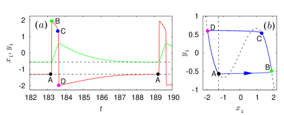
Figure 3: Blow-up of delay-induced oscillation in the first subsystem: (a) time series and (b) phase portrait $(x_{1},y_{1})$. The four different stages of the limit cycle are separated by colored dots A, B, C, D. Parameters: $\epsilon=0.01$, $a=1.3$, $C=0.5$, $\tau=3$.

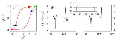
Figure 4: (a) Phase portrait of delay-coupled excitable system in the plane $(x_{1}(t),x_{2}(t-\tau))$ with positions on the orbit marked as colored dots $A,B,C,D$ as in Fig. 3. (b) Time series of $(x_{2}(t-\tau)-x_{1}(t))$. The inset shows a longer time series. Parameters: $\epsilon=0.01$, $a=1.3$, $C=0.5$, $\tau=3$.

To obtain a clear picture of the timescales involved in the dynamics, we have computed the excursion times along the segments of the phase-space trajectory. The start and end points of the different segments of the trajectory (colored dots $A$ to $D$) are defined to correspond to the time steps when the trajectory has left or entered a neighborhood $\Delta x_{1}$ (here $\Delta x_{1}\!=\!0.01$) of the stable branches of the $x_{1}$-nullcline.

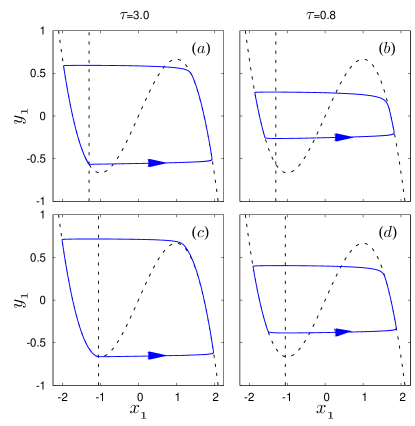
Figure 5: Phase portraits of delay-coupled excitable system $(x_{1},y_{1})$ for different excitability parameters $a$ and delay times $\tau$ (trajectories: solid blue, nullclines: dashed black). (a) $a\!=\!1.3$, $\tau\!=\!3$, (b) $a\!=\!1.3$, $\tau\!=\!0.8$, (c) $a\!=\!1.05$, $\tau\!=\!3$, (d) $a\!=\!1.05$, $\tau\!=\!0.8$. Other parameters: $\epsilon\!=\!0.01$, $C\!=\!0.5$.

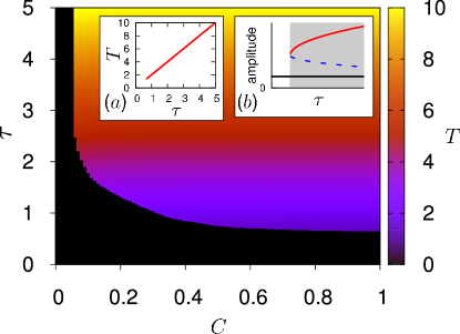
Figure 6: Regime of oscillations in the $(\tau,C)$ parameter plane for initial conditions corresponding to single-pulse-excitation in one system. The oscillation period $T$ is color coded. The transition between black and color marks the bifurcation line. Inset (a) shows the oscillation period vs. time delay $\tau$ in a cut at $C\!=\!0.8$. Parameters: $\epsilon\!=\!0.01$, $a\!=\!1.3$. Inset (b): schematic plot of the saddle-node bifurcation of a stable (red solid line) and unstable (blue dashed) limit cycle. The maximal oscillation amplitude is plotted vs. the delay time $\tau$ and the stable fixed point is plotted as a solid black line. The gray background marks the bistable region.

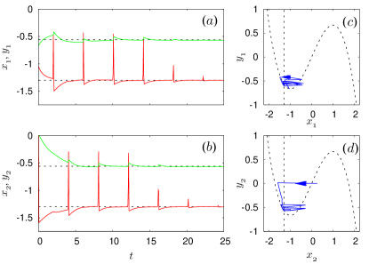
Figure 7: Unstable delay-induced limit cycle. (a), (b): Time series of both subsystems (red solid lines: activator $x_{i}$, green solid lines: inhibitor $y_{i}$; black dashed lines: fixed point value of activator and inhibitor). (c),(d): phase portraits of $(x_{1}\!,\!y_{1})$ (top) and $(x_{2}\!,\!y_{2})$ (bottom). The unstable small-amplitude limit cycle is visualized by the initial part of the transient approaching the stable fixed point. Parameters: $\epsilon\!=\!0.01$, $a\!=\!1.3$, $C\!=\!0.5$, $\tau\!=\!3$.

In the example shown in Fig. 3 ($\epsilon\!=\!0.01$, $a\!=\!1.3$, $C\!=\!0.5$, $\tau\!=\!3$) the value of the effective time shift is $\delta\!=\!0.012$. This value is about one third of the fast transition times between the stable branches of the $x_{1}$-nullcline, $\Delta t_{1}\!=\!0.041$ and $\Delta t_{3}\!=\!0.038$, respectively. $\Delta t_{1}$ is the rise-time of the spike, i.e., the time that elapses between leaving the fixed point (black dot $A$) and crossing the right stable branch of the $x_{1}$-nullcline at $B$ (green dot, Fig. 3(b)). $\Delta t_{3}$ is the drop-time, i.e., the duration of the jump back from the right to the left stable branch of the $x_{1}$-nullcline (between blue and magenta dots, $C\to D$). The slow parts of the trajectory, occurring on the right ($B\to C$) and left ($D\to A$) stable branches of the $x_{1}$-nullcline, have a duration $\Delta t_{2}\!=\!0.357$ and $\Delta t_{4}\!=\!5.588$, respectively. The total oscillation period is thus $T\!=\!6.024$.

In Fig. 5 the phase portraits of the first of the two delay-coupled subsystems are shown for different excitability parameters $a$ and delay times $\tau$. The top panel (a,b) corresponds to excitability parameters far from the Hopf bifurcation of the uncoupled system, which occurs at $a\!=\!1$. The bottom panel (c,d) corresponds to values of $a$ close to the Hopf bifurcation.

In the case of $a\!=\!1.3$ and $\tau=3$ (Fig. 5(a)), the oscillation period $T\!=\!6.024$ is large enough for the two subsystems to nearly approach the fixed point before being perturbed again by the remote signal. Note that Fig. 5(a) corresponds to Fig. 3(b). If the delay time becomes much smaller, e. g., for $\tau\!=\!0.8$ (Fig. 5 (b)), the excitatory spike of the other subsystem arrives while the first system is still in the refractory phase, so that it cannot complete the return $D\to A$ to the fixed point. The times spent in the different stages of the limit cycle for $\tau\!=\!0.8$ are $\Delta t_{1}\!=\!0.087$, $\Delta t_{2}\!=\!0.111$, $\Delta t_{3}\!=\!0.085$, and $\Delta t_{4}\!=\!1.355$, and the oscillation period is $T\!=\!1.637$. The effective time shift $\delta\!=\!0.018$ for $\tau\!=\!0.8$ is larger than for $\tau\!=\!3$.

We now investigate the transition from large to small delay times $\tau$ close to the Hopf bifurcation at $a\!=\!1.05$. Again we choose $\tau\!=\!3$ (Fig. 5(c)) and find $T\!=\!6.018$ and $\delta\!=\!0.009$. The times spent in the different phases of the oscillation period $T$ are $\Delta t_{1}\!=\!0.043$, $\Delta t_{2}\!=\!0.329$, $\Delta t_{3}\!=\!0.186$, and $\Delta t_{4}\!=\!5.461$. For the shorter delay time $\tau\!=\!0.8$ (Fig. 5(d)) we find $T\!=\!1.630$, $\delta\!=\!0.015$, $\Delta t_{1}\!=\!0.072$, $\Delta t_{2}\!=\!0.240$, $\Delta t_{3}\!=\!0.070$, and $\Delta t_{4}\!=\!1.249$. We find the same pattern as far from the Hopf bifurcation. The effective time shift $\delta$ is smaller if $\tau$ becomes larger and the system can approach the fixed point. Furthermore, if the system is close to the Hopf bifurcation and $\tau$ is sufficiently large so that the fixed point is very closely approached, $\delta$ becomes much smaller than far from the Hopf bifurcation, and tends to zero for $a\to 1$. The reason is that when the excitatory spike arrives in the first subsystem, there is a turn-on delay $\delta$ before the first subsystem emits a spike. This is because the trajectory has to cross the middle branch of the $x_{1}$-nullcline due to this upstream impulse. This section of the trajectory becomes the smaller, the closer the fixed point $A$ (at $x_{1}\!=\!-a$) is to the minimum of the $x_{1}$ nullcline (at $x_{1}\!=\!-1$). This also explains the origin of the time-shift $\delta$.

Finally, we shall investigate the question whether the system exhibits bistability between the fixed point and the limit cycle oscillation for all values of $\tau$. In Fig. 6 the regime of oscillations is shown in the parameter plane of the coupling strength $C$ and coupling delay $\tau$. The oscillation period is color coded. The boundary of this colored region is given by the minimum coupling delay $\tau_{min}$ as a function of $C$. For large coupling strength $\tau_{min}$ is almost independent of $C$; with decreasing $C$ it sharply increases, and at some minimum $C$ no oscillations exist at all. At the boundary, the oscillation sets in with finite frequency and amplitude as can be seen in the inset of Fig. 6 which shows a cut of the parameter plane at $C\!=\!0.8$. The oscillation period increases linearly with $\tau$. The mechanism that generates the oscillation is a saddle-node bifurcation of limit cycles (see Fig. 6 inset (b)), creating a pair of a stable and an unstable limit cycle. The unstable limit cycle can be visualized from transients starting at appropriate initial conditions (see Fig. 7). The trajectory initially remains near the unstable limit cycle, which separates the two attractor basins of the stable limit cycle and the stable fixed point, and then asymptotically approaches the stable fixed point.

V Conclusion

We have shown that delayed coupling can induce periodic spiking in a compound system of two coupled neuron populations if the delay and the coupling strength are sufficiently large. Bistability of a fixed point and limit cycle oscillations occur even though the single excitable element displays only a stable fixed point. The two neural populations oscillate with a phase lag of $\pi$.

VI Acknowledgements

This work was supported by DFG in the framework of Sfb 555. The authors would like to thank P. Hövel, V. Flunkert, S. Brandstetter, J. Hofmann and F. Schneider for fruitful discussions.

References

- (1) H. Haken: Brain Dynamics: Synchronization and Activity Patterns in Pulse-Coupled Neural Nets with Delays and Noise (Springer Verlag GmbH, Berlin, 2006).
- (2) H. R. Wilson: Spikes, Decisions, and Actions: The Dynamical Foundations of Neuroscience (Oxford University Press, Oxford, 1999).
- (3) W. Gerstner and W. Kistler: Spiking neuron models (Cambridge University Press, Cambridge, 2002).
- (4) H. R. Wilson and J. D. Cowan: Excitatory and inhibitory interactions in localized populations of model neurons., Biophysical journal 12, 1 (1972).
- (5) A. Destexhe, D. Contreras, T. J. Sejnowski, and M. Steriade: A model of spindle rhythmicity in the isolated thalamic reticular nucleus, J. Neurophysiol. 72, 803 (1994).
- (6) C. Zhou, L. Zemanova, G. Zamora, C. C. Hilgetag, and J. Kurths: Hierarchical organization unveiled by functional connectivity in complex brain networks, Phys. Rev. Lett. 97, 238103 (2006).
- (7) M. G. Rosenblum and A. Pikovsky: Controlling synchronization in an ensemble of globally coupled oscillators, Phys. Rev. Lett. 92, 114102 (2004).
- (8) O. V. Popovych, C. Hauptmann, and P. A. Tass: Effective desynchronization by nonlinear delayed feedback, Phys. Rev. Lett. 94, 164102 (2005).
- (9) M. Gassel, E. Glatt, and F. Kaiser: Time-delayed feedback in a net of neural elements: Transitions from oscillatory to excitable dynamics, Fluct. Noise Lett. 7, L225 (2007).
- (10) M. G. Rosenblum, A. Pikovsky, and J. Kurths: Synchronization – A universal concept in nonlinear sciences (Cambridge University Press, Cambridge, 2001).
- (11) B. Hauschildt, N. B. Janson, A. G. Balanov, and E. Schöll: Noise-induced cooperative dynamics and its control in coupled neuron models, Phys. Rev. E 74, 051906 (2006).
- (12) P. Hövel, M. A. Dahlem, and E. Schöll: Synchronization of noise-induced oscillations by time-delayed feedback, in Proc. 19th Internat. Conf. on Noise and Fluctuations (ICNF-2007) (American Institute of Physics, College Park, Maryland 20740-3843, 2007).
- (13) R. FitzHugh: Impulses and physiological states in theoretical models of nerve membrane, Biophys. J. 1, 445 (1961).
- (14) J. Nagumo, S. Arimoto, and S. Yoshizawa.: An active pulse transmission line simulating nerve axon., Proc. IRE 50, 2061 (1962).
- (15) B. Lindner, J. García-Ojalvo, A. Neiman, and L. Schimansky-Geier: Effects of noise in excitable systems, Phys. Rep. 392, 321 (2004).
- (16) N. Buric and D. Todorovic: Dynamics of fitzhugh-nagumo excitable systems with delayed coupling, Phys. Rev. E 67, 066222 (2003).
- (17) D. J. Pinto and G. B. Ermentrout: Spatially structured activity in synaptically coupled neuronal networks: I. traveling fronts and pulses, SIAM Journal on Applied Mathematics 62, 206 (2001).
- (18) S. Coombes, G. J. Lord, and M. R. Owen: Waves and bumps in neuronal networks with axo-dendritic synaptic interactions, Physica D: Nonlinear Phenomena 178, 219 (2003).
- (19) A. Hutt, M. Bestehorn, and T. Wennekers: Pattern formation in intracortical neuronal fields, Network: Computation in Neural Systems 14, 351 (2003).
- (20) A. Hutt: Effects of nonlocal feedback on traveling fronts in neural fields subject to transmission delay, Phys. Rev. E 70, 052902 (2004).
- (21) H. R. Wilson and J. D. Cowan: A mathematical theory of the functional dynamics of cortical and thalamic nervous tissue., Kybernetik 13, 55 (1973).
- (22) S. Amari: Dynamics of pattern formation in lateral-inhibition type neural fields, Biol. Cybern. 27, 77 (1977).
- (23) B. van der Pol: On relaxation oscillations, Phil. Mag. 2, 978 (1926).
- (24) B. van der Pol and J. van der Mark: The heart beat considered as a relaxation oscillation and an electrical model of the heart, Arch. Neerl. Physiol. 14, 418 (1929).
- (25) K. F. Bonhoeffer: Activation of passive iron as a model for the excitation of nerve, J. Gen. Physiol. 32, 69 (1948).
- (26) M. G. Rosenblum and A. Pikovsky: Delayed feedback control of collective synchrony: An approach to suppression of pathological brain rhythms, Phys. Rev. E 70, 041904 (2004).
- (27) E. Schöll and H. G. Schuster (Editors): Handbook of Chaos Control (Wiley-VCH, Weinheim, 2008).
- (28) N. B. Janson, A. G. Balanov, and E. Schöll: Delayed feedback as a means of control of noise-induced motion, Phys. Rev. Lett. 93, 010601 (2004).
- (29) A. G. Balanov, N. B. Janson, and E. Schöll: Control of noise-induced oscillations by delayed feedback, Physica D 199, 1 (2004).
- (30) T. Prager, H. P. Lerch, L. Schimansky-Geier, and E. Schöll: Increase of coherence in excitable systems by delayed feedback, J. Phys. A 40, 11045 (2007).
- (31) N. B. Janson, A. G. Balanov, and E. Schöll: Control of noise-induced dynamics, in Handbook of Chaos Control, edited by E. Schöll and H. G. Schuster (Wiley-VCH, Weinheim, 2008).