Rapidly Spinning Black Holes in Quasars: An Open Question

Abstract

Wang et al. (2006) estimated an average radiative efficiency of 30%–35% for quasars at moderate redshift. We find that their method is not independent of quasar lifetimes and thus that quasars do not necessarily have such high efficiencies. Nonetheless, it is possible to derive interrelated constraints on quasar lifetimes, Eddington ratios, and radiative efficiencies of supermassive black holes. We derive such constraints using a statistically complete sample of quasars with black hole mass estimates from broad Mg II, made both with and without the radiation pressure correction of Marconi et al. (2008). We conclude that for quasars with $L/L_{Edd}\gtrsim 0.02$, lifetimes can range from 140 to 750 Myr for Schwarzschild black holes. Coupled with observed black hole masses, quasar lifetimes of $\leq$140 Myr would imply that radiatively inefficient accretion or BH mergers must be important in the accretion history of quasars. Given reasonable assumptions about the quasar population, if the average quasar lifetime is $<1$ Gyr, and if radiatively inefficient accretion is unimportant, then not many BHs with Eddington ratio $<0.2$ can be rapidly spinning.

1 Introduction

A quasar is powered by matter accreting onto a supermassive black hole (e.g., Rees 1984). Gas orbiting in the innermost stable circular orbit (ISCO) may be perturbed and fall into the black hole (BH), adding mass and angular momentum to it. To have reached the ISCO through a thin accretion disk, gas must have radiated away a fractional binding energy per unit rest mass $\simeq 1-(1-2GM/3c^{2}R_{ISCO})^{1/2}$ which is the system’s radiative efficiency $\eta$ (Bardeen 1970). Since $R_{ISCO}$ decreases from $6GM/c^{2}$ for Schwarzschild (nonrotating) BHs to $GM/c^{2}$ for co-aligned accretion onto Extreme-Kerr (maximally rotating) BHs, more energy is produced by (co-aligned) thin disk accretion of a given mass onto a rotating BH than onto a non-rotating BH (Carter 1968).

If a quasar accretes gas with a fixed angular momentum vector at a fixed mass accretion rate $\dot{M}$, the BH spin will increase to a theoretical maximum and the luminosity $L$ of the quasar will increase along with it, since $L\propto\eta\dot{M}c^{2}$. In many realistic accretion models, the spin of a supermassive BH increases rapidly and then fluctuates around a maximum value, although spin-down is also possible (Volonteri 2007). Several such models, including numerical ones by Di Matteo et al. (2005), suggest that the accretion process stops when a BH becomes massive enough to support a kinetic and/or radiative luminosity capable of blowing away the gas fuelling it (Silk & Rees 1998; Fabian 1999; King 2003). However, the radiative luminosity for a given mass accretion rate depends upon the radiative efficiency. A rapidly rotating BH can help shut down the accretion process earlier than a nonrotating BH could. Knowledge of supermassive BH spins is therefore useful in constraining models of quasar development.

Observationally, the quasi-periodic variability detected in Sgr A* may be evidence of rapid spin of the Galactic BH (e.g., Genzel et al. 2003). Evidence for rotating supermassive BHs comes from studies of X-ray Fe K$\alpha$ line profiles (Blandford et al. 1990) and by theoretical arguments that powerful radio jets are powered by the extraction of energy from rotating BHs (Miller 2007).

In a recent study, Wang et al. (2006; hereafter WCHM) estimated a high average radiative efficiency of 30%–35% for quasars at $0.4<z<2.1$, implying that most supermassive black holes are rapidly rotating. However, the existence of rotating BHs with $\eta\gtrsim 0.18$ is not confirmed by magnetohydronamic (MHD) simulations: gas loses more angular momentum prior to accretion in an MHD disk than in a standard thin disk (Gammie & Shapiro 2004; Shapiro 2005). Observationally, Shankar et al. (2008) present and review evidence for $\eta\lesssim 0.1$. In this work we show that the WCHM method is not independent of quasar lifetimes. In § 2 we correct and extend the WCHM method for determining radiative efficiencies, in § 3 we apply it to a sample of Sloan Digital Sky Survey (SDSS) quasars and in § 4 we discuss our conclusions.

2 The Method:

We assume that quasar light derives only from accretion of matter onto a black hole, neglecting the effects of BH mergers. Suppose that mass propagates through a thin accretion disk around an accreting BH at a rate of $\dot{M}_{acc}$ during some time interval of $\Delta t$. The BH mass growth rate is given by $\dot{M}=(1-\eta)\dot{M}_{acc}$, where $\eta$ is the radiative efficiency. The quasar radiates at bolometric luminosity $L$ (Marconi et al. 2004) given by:

$$L\Delta t=\eta\dot{M}_{acc}c^{2}\Delta t=\frac{\eta}{1-\eta}\dot{M}c^{2}\Delta t.$$ (1)

We can rewrite the above equation as:

$$\eta={L\Delta t\over L\Delta t+\dot{M}c^{2}\Delta t}\equiv{\delta\epsilon\over\delta\epsilon+\delta\rho c^{2}}$$ (2)

where $\delta\epsilon\equiv L\Delta t/V_{com}$ is the change over the time $\Delta t$ in the comoving radiative energy density and $\delta\rho\equiv\dot{M}\Delta t/V_{com}$ is the accompanying change in the comoving BH mass density, both due solely to this BH’s accretion.

By analogy, an average radiative efficiency can be defined for any sample of quasars at redshift $z$:

$$\bar{\eta}(z)\equiv\frac{\Delta\varepsilon(z)}{\Delta\varepsilon(z)+\Delta\varrho(z)c^{2}}$$ (3)

where $\Delta\varepsilon(z)$ and $\Delta\varrho(z)$ are the estimated changes in the cumulative radiative energy density and the cumulative mass density of the sample in the redshift range $(z,z+\Delta z)$. We now define these cumulative densities.

We require the quasar black hole mass function $n(M,z)$, defined such that $n(M,z)~{}\Delta M~{}\Delta z$ is the comoving number density of black holes with masses in the range ($M,M+\Delta M$) in the redshift range $(z,z+\Delta z)$. We also require the quasar bolometric luminosity function $\psi(L,z)$, where $\psi(L,z)~{}\Delta L~{}\Delta z$ is the comoving number density of black holes with bolometric luminosity in the range ($L,L+\Delta L$) in the redshift range $(z,z+\Delta z)$.

Over its lifetime $t_{q}$, a single quasar accretes a mass $M_{final}$=$\dot{M}_{avg}t_{q}$ and radiates an energy $L_{avg}t_{q}$. We need to express those quantities in terms of the observables $M_{i}$ and $L_{j}$, which are the black hole’s mass and bolometric luminosity at the redshift of observation, $z$. We do so by defining correction factors $\bar{f}$ and $\bar{g}$ such that

$$\bar{f}={1\over N}\sum_{i=1}^{N}{M_{i}\over M_{final,i}}=\left<{M_{i}\over M_{final,i}}\right>~{}~{}{\rm and}~{}~{}\bar{g}={1\over N}\sum_{j=1}^{N}{L_{j}\over L_{avg,j}}=\left<{L_{j}\over L_{avg,j}}\right>$$ (4)

where the averages are over all $N$ quasars in the sample.

First, consider the mass density that contributes to Eq. 3. Over their lifetimes, all black holes observed at redshift $z$ will accrete a comoving matter density of

$$\sum_{M_{i}}n(M_{i},z)M_{final}\Delta M_{i}=\sum_{M_{i}}n(M_{i},z)M_{i}\Delta M_{i}/\bar{f}.$$ (5)

The cumulative, lifetime amount of matter accreted by all black holes observed at $\geq$$z$ and above is the comoving lifetime mass density summed over all redshifts $\geq$$z$:

$$\varrho(z)=\sum_{z_{k}>z}\Delta\varrho(z_{k})=\sum_{z_{k}>z}\Delta z_{k}\sum_{M_{i}}n(M_{i},z_{k})M_{i}\Delta M_{i}/\bar{f}$$ (6)

which agrees with Eqs. 2 and 6 of WCHM if $\bar{f}=1$. Notice that units of $\Delta\varrho/\Delta z$ are mass per comoving volume per redshift.

Now consider the radiative energy component of Eq. 3. Over their lifetimes, all black holes observed at redshift $z$ will radiate a comoving energy density of

$$\sum_{L_{j}}\psi(L_{j},z)L_{avg}\bar{t}_{q}\Delta L_{j}=\sum_{L_{j}}\psi(L_{j},z)L_{j}\bar{t}_{q}\Delta L_{j}/\bar{g},$$ (7)

where $\bar{t}_{q}$ is the average quasar lifetime. The cumulative, lifetime amount of energy radiated by all black holes observed at redshift $z$ and above is the comoving lifetime energy density summed over all redshifts above $z$:

$$\varepsilon(z)=\sum_{z_{k}>z}\Delta\varepsilon(z_{k})=\sum_{z_{k}>z}\Delta z_{k}\sum_{L_{j}}\psi(L_{j},z_{k})L_{j}\bar{t}_{q}\Delta L_{j}/\bar{g}$$ (8)

which differs from Eqs. 3 and 5 of WCHM. Their expression for $\Delta\varepsilon(z)$ is a factor of $\Delta t_{k}/\Delta z_{k}\bar{t}_{q}$ times the true value above (assuming $\bar{g}=1$), where $\Delta t_{k}$ is the cosmological time spanned by the redshift interval $\Delta z_{k}$. The units of $\Delta\varepsilon/\Delta z$ above are energy per comoving volume per redshift, whereas in Eq. 5 of WCHM they are energy per comoving volume per (redshift)², which is incorrect.

The first quantity of interest, the change in the cumulative comoving mass density of actively accreting black holes over the redshift range $(z,z+\Delta z)$ — $\Delta\varrho(z)$ — is $\Delta z$ times the sum of the masses of all individual quasar black holes in the sample in that $z$ range, divided by the comoving volume:

$$\Delta\varrho(z)=\Delta z~{}\sum_{M_{i}}n(M_{i},z)~{}M_{i}~{}\Delta M_{i}/\bar{f}.$$ (9)

In other words, the change in the cumulative comoving mass density in the redshift bin $(z,z+\Delta z)$, which is $\Delta\varrho(z)/\Delta z$, is the same as the comoving mass density in that bin. Similarly, the second quantity of interest, the change over the redshift range $(z,z+\Delta z)$ in the cumulative radiative energy density ever observed from all quasars — $\Delta\varepsilon(z)$ — is

$$\Delta\varepsilon(z)=\Delta z~{}\sum_{L_{j}}\psi(L_{j},z)~{}L_{j}~{}\Delta L_{j}~{}\bar{t}_{q}/\bar{g}.$$ (10)

These expressions for $\Delta\varrho(z)$ and $\Delta\varepsilon(z)$ can be substituted into Eq. 3 to find $\bar{\eta}(z)$ for the sample of quasars under consideration. Doing so, and grouping $\bar{t}_{q}$, $\bar{f}$ and $\bar{g}$ together, we obtain:

$$\bar{\eta}(z)={\displaystyle\sum_{L_{j}}\psi(L_{j},z)~{}L_{j}~{}\Delta L_{j}\over\displaystyle\sum_{L_{j}}\psi(L_{j},z)~{}L_{j}~{}\Delta L_{j}+{\bar{g}c^{2}\over\bar{f}\bar{t}_{q}}\displaystyle\sum_{M_{i}}n(M_{i},z)~{}M_{i}~{}\Delta M_{i}}$$ (11)

where the $\Delta z$ in the numerator and denominator have cancelled out, making the calculation independent of $\Delta z$ even if $\bar{t}_{q}$ is longer than the cosmic time interval corresponding to $\Delta z$.

Thus, the WCHM method for studying radiative efficiencies is not independent of the average quasar lifetime $\bar{t}_{q}$. A factor of $\bar{t}_{q}$ enters because both the mass-energy growth and the radiative energy output of a quasar must be summed over its entire lifetime (or over the same portion of its lifetime). The mass-energy sum yields the final mass-energy of the black hole $M_{tot}c^{2}$, while the radiative energy sum yields $L_{avg}\bar{t}_{q}$. However, this method remains independent of obscured sources and is also powerful because it can be implemented for any sample of quasars regardless of selection effects. It requires only that the changes in the cumulative mass-energy and radiative energy densities be computed using the same objects. Of course, selection effects will determine if the resulting radiative efficiency is relevant for quasars in general.

Also, WCHM in effect assumed $\bar{f}=\bar{g}=1$. We adopt more realistic estimates by examining Fig. 14 of Springel et al. (2005) and Fig. 1 of Hopkins et al. (2005), from which we respectively estimate $\bar{f}\simeq 1$ and $\bar{g}\simeq 10$ for those models. Adopting $\bar{f}$=1 means that a quasar is observed when its black hole has accumulated essentially all of its mass, while $\bar{g}$=10 means that the observed bolometric luminosity of a quasar is around 10 times larger than the average luminosity of a quasar throughout its entire life. Our value of $\bar{g}$ is estimated by averaging $L_{j}/L_{ave}$ over the period of time when quasar shows its final burst of activity (between 1.2 to 1.4 Gyr in Fig. 1 of Hopkins et al. 2005).

If WCHM had assumed $\bar{f}=1$ and $\bar{g}=10$, we estimate that their (incorrect) calculation would have yielded $\eta\lesssim 0.1$ instead of $\eta\simeq 0.32$. However, Eq. 11 shows that even with realistic $\bar{f}$ and $\bar{g}$ values the average quasar radiative efficiency is dependent on the average quasar lifetime. We now explore the implications of this dependency.

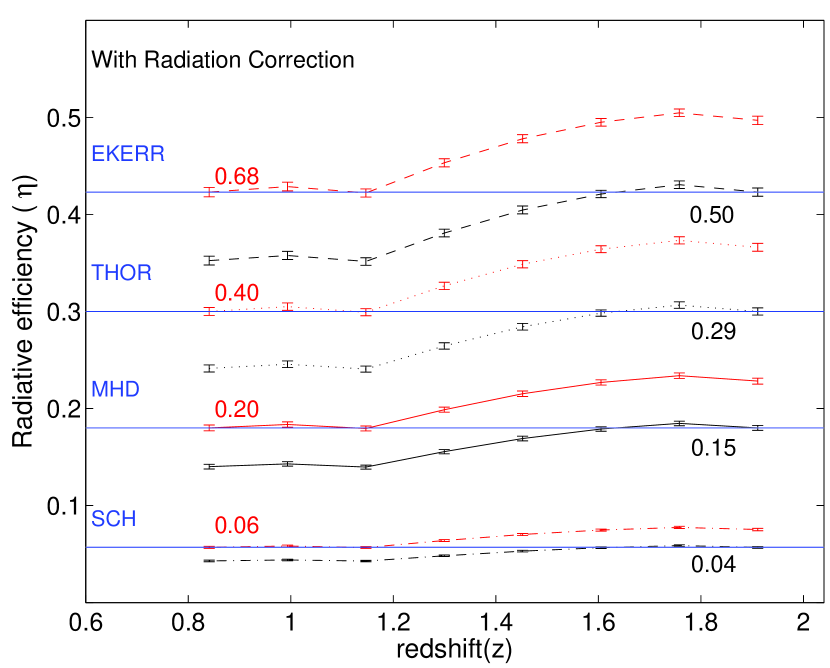
Figure 1: Tracks of putative radiative efficiency $\eta$ vs. redshift z for different assumed values of the quasar lifetime in Gyr, all assuming $\bar{f}=\bar{g}=1$. The blue horizontal lines show $\eta$ for the Extreme-Kerr BH limit (EKERR), the Thorne BH limit (THOR), the magnetohydrodynamic BH limit (MHD) and the Schwarzschild BH limit (SCH) respectively. The assumed quasar lifetimes are given next to each track, on the left for tracks chosen to match a particular radiative efficiency line at low redshift epochs and on the right for high redshift epochs. An Extreme-Kerr BH with $\bar{t}_{q}\simeq 0.68$ Gyr at $z\simeq 0.9$ would violate the maximum possible radiative efficiency at $z\simeq 2$. This inconsistency indicates the existence of a hidden parameter; namely, Eddington ratio which is considered in Figure 2.

3 Application to SDSS Quasars

3.1 Estimation of Black Hole Masses and Bolometric Luminosity

Based on reverberation mapping studies of local active galaxies, an empirical scaling relationship has been developed to estimate black hole masses by (e.g.) Kaspi et al. (2000), Vestergaard (2002) and McLure et al. (2002). The Sloan Digital Sky Survey (York et al. 2000) Data Release 3 quasar catalog (Schneider et al. 2005) provides us with a large sample of quasars at redshifts $0.7<z<2.1$ which have their Mg II $\lambda$2800 emission line redshifted into the SDSS spectral range. We have estimated black hole masses for 27728 such quasars from the dispersion of the Mg II emission line and the continuum luminosity at $\lambda$=3000 Å and for two scenarios. Scenario A: we assume that a black hole mass can be estimated from a conventional virial relationship as: $M_{BH}/M_{\odot}=30.5[\lambda L_{\lambda}]^{0.5}\sigma_{\rm Mg}^{2}$ where $L_{\lambda}$ has units of $10^{44}$ erg s^-1 and $\sigma_{\rm Mg}$ km s^-1. Scenario B: we follow Marconi et al. (2008) in considering the effect of the radiation pressure of the quasar’s radiation on black hole mass estimates, namely that it reduces the effective gravity on the broad emission line region, yielding narrower lines at a given mass. We adopt the BH mass relationship with this radiation correction to be: $M_{BH}/M_{\odot}=5.75\bar{\zeta}_{\sigma}[\lambda L_{\lambda}]^{0.5}\sigma_{\rm Mg}^{2}+\bar{\xi}_{\sigma}~{}[\lambda L_{\lambda}]$ where $\bar{\zeta}_{\sigma}=2.4\pm 1.5$ and log$\bar{\xi}_{\sigma}=6.9\pm 0.5$ (Rafiee et al. 2008, in prep.).

Furthermore a Malmquist-like bias has been estimated following § 4 of Shen et al. (2008). Our black hole mass estimates have been adjusted downward by a mean bias of $0.4$ dex for scenario A and $0.11$ dex for scenario B, arising from the steepness of the BH mass function and the scatter in BH mass estimates.

We have matched our sample with that of Richards et al. (2006a), a homogeneously selected and statistically complete sample of 15343 DR3 quasars with redshifts $z<5$ drawn from an effective area of 1622 $\textmd{deg}^{2}$. This procedure yields a subsample of 6704 quasars. The bolometric luminosities of these quasars have been estimated from $L_{bol}=C_{\lambda}\lambda L_{\lambda}$ with $C_{\lambda}=5.15$ for $\lambda$=3000 Å following Shen et al. 2008.

Comoving volumes and luminosity distances have been calculated using a $\Lambda$CDM cosmology with $h=0.71$, $\Omega_{\Lambda}=0.74$ and $\Omega_{m}=0.26$ (Spergel at al. 2007). Corrections have been made for the limited areal coverage of the Richards et al. (2006a) sample and for the 5% incompleteness of the SDSS at $0.7<z<2.1$. For more details, see Fig. 8 of Richards et al. (2006a).

3.2 Radiative Efficiency and Redshift Binning

For thin accretion disks, the only disks we consider in this paper, $\eta$ varies from $0.057$ for a Schwarzschild BH (with $a^{\ast}\equiv Jc/GM^{2}=0$, where $J$ is the angular momentum) to $0.42$ for an Extreme-Kerr BH ($a^{\ast}=1$). When one takes into account the effect of radiation energy captured by the BH (Thorne 1974), the radiative efficiency reaches a maximum of $\simeq 0.30$ ($a^{\ast}\simeq 0.998$); we refer to that case as a Thorne BH. It is more realistic to assume an MHD disk wherein magnetic turbulence provides a torque to remove angular momentum from the inflowing gas (Shapiro 2005); in that case, the maximum radiative efficiency is $\simeq 0.18$ ($a^{\ast}\simeq 0.938$).

We divide our sample into twelve redshift bins. In each bin we can compute $\eta$ for any given value of $\bar{t}_{q}$. The results are shown in Figure 1 as tracks of $\eta(z)$ for eight different values of $\bar{t}_{q}$ chosen to match the $\eta$ of a Schwarzschild, MHD, Thorne or Extreme-Kerr black hole at either the high or low redshift limit of our sample. Figure 1 is the corrected version of Figure 2 of WCHM. Both figures show the evolution of $\eta$ with $z$ for a flux-limited quasar sample, assuming constant $\bar{t}_{q}$. However, this figure does not give a complete picture since there is another degree of freedom not being considered; namely, the Eddington ratios of the quasars. For example, taken at face value, Figure 1 suggests that a quasar with a lifetime of 0.68 Gyr can be powered by a Extreme-Kerr BH at $z\simeq 0.9$ while the same quasar would violate the maximum possible radiative efficiency at $z\simeq 2$. Since quasars in our sample have larger values of the Eddington ratio at $z\simeq 2$ than at $z\simeq 0.8$, the trend in Figure 1 might be explained by the importance of the Eddington ratio rather than the redshift.

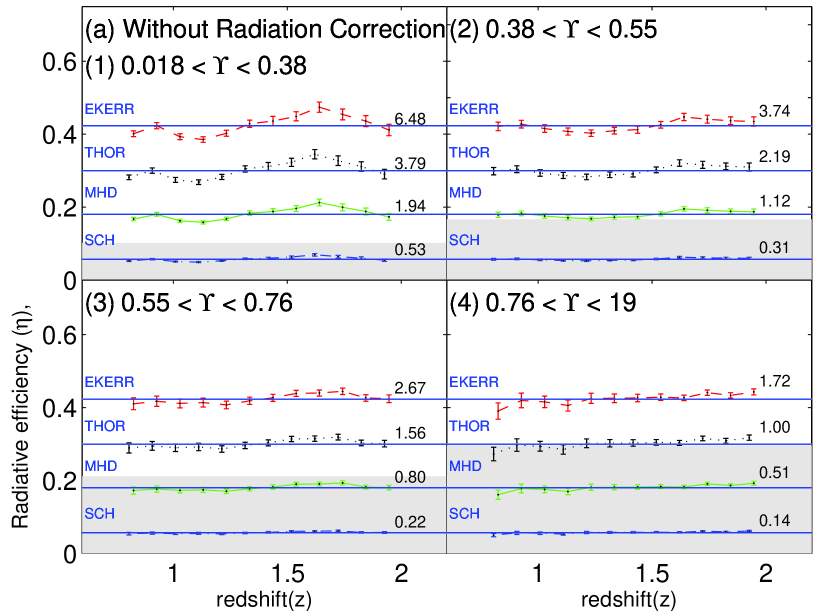
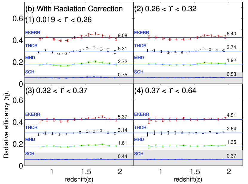
Figure 2: Radiative efficiencies vs. $z$ for different Eddington ratio bins and constant assumed quasar lifetimes in Gyr (printed in each panel for each BH type). (a) Scenario A. (b) Scenario B. Lifetimes were chosen so the resulting $\eta$ would match that of each BH type. We assume $\bar{f}=1$ and $\bar{g}=10$ — quasars are observed at their final mass and ten times their average luminosity. The shaded areas are the regions corresponding to $\bar{t}_{q}\lesssim 1$ Gyr, the possible upper limit for quasar lifetime suggested by Marconi et al. (2004).

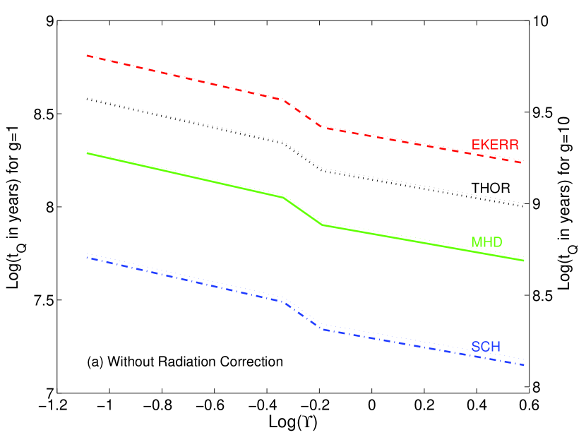
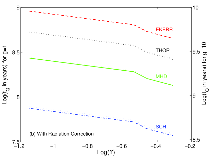
Figure 3: Quasar lifetime versus Eddington ratio. (a) Scenario A. (b) Scenario B. Quasars will lie in the area between the Schwarzschild and Thorne curves if they are described by radiatively efficient accretion disks. Below the Schwarzschild curves requires radiatively inefficient accretion or $\bar{\Upsilon}>\Upsilon_{obs}$, while above the MHD curves requires $\bar{\Upsilon}<\Upsilon_{obs}$. Left axis labels are for $\bar{f}=\bar{g}=1$; right axis labels are for $\bar{g}=10$ and $\bar{f}=1$.

3.3 Eddington Ratio Binning

We assume the radiative efficiency may be a function of the Eddington ratio $\Upsilon\equiv L_{bol}/L_{Edd}$, where $L_{Edd}=1.26\times 10^{38}(M_{BH}/M_{\odot})$ erg s^-1. In that case, the changes in the cumulative comoving mass and energy densities in the Eddington ratio bin ($\Upsilon,\Upsilon+\Delta\Upsilon$) are:

$$\Delta\varrho_{\bullet}(z,\Upsilon)=\Delta\Upsilon~{}\Delta z~{}\sum_{M_{i}}n(\Upsilon,M_{i},z)~{}M_{i}~{}\Delta M_{i}/\bar{f}.$$ (12)

$$\Delta\varepsilon_{\bullet}(z,\Upsilon)=\Delta\Upsilon~{}\Delta z~{}\sum_{L_{j}}\psi(\Upsilon,L_{j},z)~{}L_{j}~{}\Delta L_{j}~{}\bar{t}_{q}/\bar{g}$$ (13)

where $n$ and $\psi$ now depend on $\Upsilon$ as well as $z$. The bullet subscript denotes quantities binned in $\Upsilon$ as well as $z$.

The average radiative efficiency for a given $\Upsilon$ and $z$ is

$$\bar{\eta}(z,\Upsilon)=\frac{\Delta\varepsilon_{\bullet}(z,\Upsilon)}{\Delta\varepsilon_{\bullet}(z,\Upsilon)+\Delta\varrho_{\bullet}(z,\Upsilon)c^{2}}.$$ (14)

For the same sub-sample used in section 3.2 and for twelve redshift bins, ten mass bins, and ten luminosity bins, the radiative efficiency has been estimated for four different Eddington ratio bins (Figure 2), each containing one quartile of the objects. Figure 2 shows that radiative efficiency is not a function of redshift but rather of quasar lifetime and Eddington ratio.

4 Discussion and Summary

Determinations of quasar lifetimes, Eddington ratios and radiative efficiencies are interrelated. Given constraints on (or assumptions about) quasar lifetimes, the WCHM method can be used to constrain quasar radiative efficiencies and BH spins. (Without such constraints, the average quasar $\eta$ cannot be estimated by this method.) Conversely, the range of radiative efficiencies possible for the full range of BH spins can be used to constrain average quasar lifetimes, as long as luminous quasars are not powered by radiatively inefficient accretion flows (RIAFs; see, e.g., Blandford & Begelman 1999). For example, for the $\eta=0.065,\Upsilon\simeq 0.4$ model of Shankar et al. (2008), we predict $\bar{t}_{q}\simeq 140$ million years in our scenario A or $\bar{t}_{q}\simeq 370$ million years in scenario B, which could be used as a further test of those models in comparison to others.

Assuming $\bar{f}=1$ and $\bar{g}=10$ (see the end of § 2), quasar lifetimes can be constrained according to the Eddington ratio of the quasar. Lifetimes estimated this way are within a factor of a few of literature lifetime estimates. For example, for BHs in the mass range of our sample ($10^{8}$$<$$M_{BH}$$<$$10^{10}M_{\odot}$), a lower limit lifetime of 530 million years can be established for black holes with $0.02$$<$$\Upsilon$$<$$0.38$ (Panel 1 of Figure 2a, scenario A) or around 750 million years in scenario B for $0.02$$<$$\Upsilon$$<$$0.26$. This lower limit corresponds to the Schwarzschild case, since a rotating black hole at the same $\Upsilon$ will require a longer lifetime to build up its observed mass. This lower limit lifetime is less than a factor of two lower than the mean lifetime of one billion years estimated by Marconi et al. (2004) for $\Upsilon=0.1$ and $\eta=0.04$ in the same range of $M_{BH}$. As another example, a luminous quasar powered by a relatively low-mass black hole — which may be a typical early stage in a quasar’s evolution — will have $\Upsilon\gtrsim 0.4$ and can have a typical lifetime of 140 to 510 million years (Panel 4 of Figure 2a). This range is only a factor of $\sim 3$ larger than the mean lifetime of $30-130$ million years estimated by Yu & Tremaine (2002) for luminous quasars, and is consistent with the mean lifetime of $100-450$ million years estimated by Marconi et al. (2004) for super-Eddington accretors.

In principle, given constraints on $\Upsilon\propto\eta\dot{M}/(1-\eta)M_{BH}$, $\bar{f}/\bar{g}$ and $\bar{t}_{q}$ for quasar samples, one could estimate the historical frequency of RIAF episodes in those quasars by plotting quasar lifetimes versus Eddington ratios. For example, consider quasars lying below the Schwarzschild curves in Figure 3 (the normalization of which is a function of $\bar{f}/\bar{g}$, as seen by comparing the two axis in either scenario A or B). Above our lower mass limit of $10^{8}M_{\odot}$, such quasars must either have had a RIAF phase in order to explain their observed masses, or they must have observed Eddington ratios lower than their historical average: $\Upsilon_{obs}<\bar{\Upsilon}$. (In the latter case, the quasars historically would have been located horizontally to the right in the diagram, lying between the Schwarzschild and Thorne curves at a value of $\Upsilon=\bar{\Upsilon}$ sufficient to yield the observed $M_{BH}$ in the observed $\bar{t}_{q}$.) Conversely, quasars lying above the Thorne curves in Figure 3 require $\Upsilon_{obs}>\bar{\Upsilon}$. A low $\bar{\Upsilon}$ might result if the BH spin does not increase as fast as the BH mass does, perhaps due to counter-rotating gas accretion phases. If $\bar{f}=1$ and $\bar{g}=10$ and $\bar{t}_{q}<1$ Gyr, and if RIAFs are unimportant, then not many BHs with $\Upsilon<0.2$ can be rapidly spinning. On the other hand, if $\bar{f}=1$ and $\bar{g}=10$ and $\bar{t}_{q}<140$ Myr, then RIAFs or BH mergers must be important for quasars regardless of $\Upsilon$, since only then could the observed masses be reached in the inferred lifetimes.

What can we conclude if we assume that the Marconi et al. (2008) correction for the effect of radiation pressure on quasar BH masses is valid, and that $\bar{t}_{q}\leqslant 1$ Gyr (Martini et al. 2004; Marconi et al. 2004)? First of all, most quasars can not be rapidly spinning in that case. Second, most of the quasars in our sample have a radiative efficiency of $\lesssim 0.14$ consistent with the results of Yu & Tremaine (2002). This $\eta$ being lower than the MHD prediction of Shapiro (2005) might be explained by the effects of BH mergers or by the fraction of maximally spinning BHs being low, at least in our sample.

Alternatively, if one assumes thick disk accretion, where the relation between the BH spin and radiative efficiency differs from thin disk accretion, then radiatively inefficient accretion becomes more important even for MHD accretion and spinning BHs, making a lower $\eta$ more plausible.

In conclusion, the Wang et al. (2006) method, despite its advantages, can only estimate the radiative efficiency of quasars and ultimately the spin of black holes if we know enough about the accretion process and the evolutionary history of black holes. Better estimates of $\bar{f}$, $\bar{g}$ and $\bar{t}_{q}$ from ultimately, however, more detailed evolutionary models, might improve the reliability of the results. Lack of knowledge about the geometry and dynamics of the accretion disk limits the level of reliability of this method.

PBH and AR are supported in part by NSERC.

References

- (1) Bardeen, J. M. 1970, Nature, 226, 64.
- (2) Blandford, R. D., Netzer, H., Woltjer, L. Courvoisier, T. J. L., & Mayor, M. 1990, Active Galactic Nuclei (Berlin: Springer-Verlag)
- (3) Blandford, R. D. & Begelman, M. C. 1999, MNRAS, 303, L1
- (4) Carter, B. 1968, Phys. Rev., 1559
- (5) Di Matteo, T., Springel, V. & Hernquist, L. 2005, Nature, 433, 604
- (6) Fabian, A. C. 1999, MNRAS, 308, L39
- (7) Gammie, C., Shapiro, S. & McKinney, J. 2004, ApJ, 602, 312
- (8) Genzel, R., et al. 2003, Nature, 425, 934
- (9) Hopkins, P. F., et al. 2005, ApJ, 625, L71
- (10) Hopkins, P. F., et al. 2006, ApJ, 643, 641
- (11) Kaspi, S., Smith, P. S., Netzer, H., et al. 2000, ApJ, 533, 631
- (12) King, A. 2003, ApJ, 596, L27
- (13) King, A., Pringle, J., Hofmann, J. 2008, MNRAS, 385, 1621
- (14) Marconi, A., Risaliti, G., et al. 2004, MNRAS, 351, 169
- (15) Marconi, A., Axon, J. D., et al. 2008, ApJ, 678, 693
- (16) Martini, P., et al. 2003, ApJ, 597, L109
- (17) McLure, R. J. & Jarvis, M. J. 2002, MNRAS, 337, 109
- (18) Miller, J. M. 2007, ARA&A, 45:441-79
- (19) Rees, M. J. 1984, ARA&A, 22, 471
- (20) Richards, G. T., et al. 2006a, AJ, 131, 2766
- (21) Richards, G. T., et al. 2006b, ApJS, 166, 470
- (22) Schneider, D. P., et al. 2005 ApJ, 130, 367
- (23) Shankar, F., Weinberg, D. & Miraldi-Escude, J. 2008, submitted
- (24) Shapiro, S. L. 2005 ApJ, 620, 59
- (25) Shen, Yue., et al. 2008, ApJ, 680, 169
- (26) Silk, J. & Rees, M. J. 1998, A&A 331, L1
- (27) Spergel, D. N., et al. 2007, ApJS, 170, 377
- (28) Springel, V., et al. 2005, MNRAS, 361, 776
- (29) Thorne, K. S. 1974, ApJ, 191, 507
- (30) Vestergaard, M. 2002, ApJ, 571, 733
- (31) Volonteri, M. 2008, MNRAS, 383, 1079
- (32) Wang, J., Chen, Y., Ho, L. & McLure, R. 2006, 642, L111 [WCHM]
- (33) York, D. G., et al. 2000, AJ, 120, 1579
- (34) Yu, Q. & Tremaine, S. 2002, MNRAS, 335, 965