Consistent Computation of First- and Second-Order
Differential Quantities for Surface Meshes

Abstract

Differential quantities, including normals, curvatures, principal directions, and associated matrices, play a fundamental role in geometric processing and physics-based modeling. Computing these differential quantities consistently on surface meshes is important and challenging, and some existing methods often produce inconsistent results and require ad hoc fixes. In this paper, we show that the computation of the gradient and Hessian of a height function provides the foundation for consistently computing the differential quantities. We derive simple, explicit formulas for the transformations between the first- and second-order differential quantities (i.e., normal vector and principal curvature tensor) of a smooth surface and the first- and second-order derivatives (i.e., gradient and Hessian) of its corresponding height function. We then investigate a general, flexible numerical framework to estimate the derivatives of the height function based on local polynomial fittings formulated as weighted least squares approximations. We also propose an iterative fitting scheme to improve accuracy. This framework generalizes polynomial fitting and addresses some of its accuracy and stability issues, as demonstrated by our theoretical analysis as well as experimental results.

I.3.5Computer GraphicsComputational Geometry and Object ModelingAlgorithms, Design, Experimentation

1 Introduction

Computing normals and curvatures is a fundamental problem for many geometric and numerical computations, including feature detection, shape retrieval, shape registration or matching, surface fairing, surface mesh adaptation or remeshing, front tracking and moving meshes. In recent years, a number of methods have been introduced for the computation of the differential quantities (see e.g., [Taubin 1995, Meek and Walton 2000, Meyer et al. 2002, Cazals and Pouget 2005]). However, some of the existing methods may produce inconsistent results. For example, when estimating the mean curvature using the cotangent formula and estimating the Gaussian curvature using the angle deficit [Meyer et al. 2002], the principal curvatures obtained from these mean and Gaussian curvatures are not guaranteed to be real numbers. Such inconsistencies often require ad hoc fixes to avoid crashing of the code, and their effects on the accuracy of the applications are difficult to analyze.

The ultimate goal of this work is to investigate a mathematically sound framework that can compute the differential quantities consistently (i.e., satisfying the intrinsic constraints) with provable convergence on general surface meshes, while being flexible and easy to implement. This is undoubtly an ambitious goal. Although we may have not fully achieved the goal, we make some contributions toward it. First, using the singular value decomposition [Golub and Van Loan 1996] of the Jacobian matrix, we derive explicit formulas for the transformations between the first- and second-order differential quantities of a smooth surface (i.e., normal vector and principal curvature tensor) and the first- and second-order derivatives of its corresponding height function (i.e., gradient and Hessian). We also give the explicit formulas for the transformations of the gradient and Hessian under a rotation of the coordinate system. These transformations can be obtained without forming the shape operator and the associated computation of its eigenvalues or eigenvectors. We then reduce the problem, in a consistent manner, to the computation of the gradient and Hessian of a function in two dimensions, which can then be computed more readily by customizing classical numerical techniques.

Our second contribution is to develop a general and flexible method for differentiating a height function, which can be viewed as a generalization of the polynomial fitting of osculating jets [Cazals and Pouget 2005]. Our method is based on the Taylor series expansions of a function and its derivatives, then solved by a weighted least squares formulation. We also propose an iterative-fitting method that improves the accuracy of fittings. Furthermore, we address the numerical stability issues by a systematic point-selection strategy and a numerical solver with safeguard. We present experimental results to demonstrate the accuracy and stability of our approach for fittings up to degree six.

The remainder of this paper is organized as follows. Section 2 reviews some related work on the computation of differential quantities of discrete surfaces. Section 3 analyzes the stability and consistency of classical formulas for computing differential quantities for continuous surfaces and establishes the theoretical foundation for consistent computations using a height function. Section 4 presents a general framework and a unified analysis for computing the gradient and Hessian of a height function based on polynomial fittings, including an iterative-fitting scheme. Section 5 presents some experimental results to demonstrate the accuracy and stability of our approach. Section 6 concludes the paper with a discussion on future research directions.

2 Related Work

Many methods have been proposed for computing or estimating the first- and second-order differential quantities of a surface. In recent years, there have been significant interests in the convergence and consistency of these methods. We do not attempt to give a comprehensive review of these methods but consider only a few of them that are more relevant to our proposed approach; readers are referred to [Petitjean 2002] and [Gatzke and Grimm 2006] for comprehensive surveys. Among the existing methods, many of them estimate the different quantities separately of each other. For the estimation of the normals, a common practice is to estimate vertex normals using a weighted average of face normals, such as area weighting or angle weighting. These methods in general are only first-order accurate, although they are the most efficient.

For curvature estimation, Meyer et al. MDSB02DDG proposed some discrete operators for computing normals and curvatures, among which the more popular one is the cotangent formula for mean curvatures, which is closely related to the formula for Dirichlet energy of Pinkall and Polthier PP93CDM. Xu Xu04CDL studied the convergence of a number of methods for estimating the mean curvatures (and more generally, the Laplace-Beltrami operators). It was concluded that the cotangent formula does not converge except for some special cases, as also noted in [Hildebrandt et al. 2006, Wardetzky 2007]. Langer et al. LBS05ADD,LBS05EAQ proposed a tangent-weighted formula for estimating mean-curvature vectors, whose convergence also relies on special symmetric patterns of a mesh. Agam and Tang AT05SFA proposed a framework to estimate curvatures of discrete surfaces based on local directional curve sampling. Cohen-Steiner and Morvan CM03RDT used normal cycle to analyze convergence of curvature measures for densely sampled surfaces.

Vertex-based quadratic or higher-order polynomial fittings can produce convergent normal and curvature estimations. Meek and Walton MW00SNG studied the convergence properties of a number of estimators for normals and curvatures. It was further generalized to higher-degree polynomial fittings by Cazals and Pouget CP05EDQ. These methods are most closely related to our approach. It is well-known that these methods may encounter numerical difficulties at low-valence vertices or special arrangements of vertices [Lancaster and Salkauskas 1986], which we address in this paper. Razdan and Bae RB05CES proposed a scheme to estimate curvatures using biquadratic Bézier patches. Some methods were also proposed to improve robustness of curvature estimation under noise. For example, Ohtake et al. OBS04RVL estimated curvatures by fitting the surface implicitly with multi-level meshes. Recently, Yang et al. YLHP06RPC proposed to improve robustness by adapting the neighborhood sizes. These methods in general only provide curvature estimations that are meaningful in some average sense but do not necessarily guarantee convergence of pointwise estimates.

Some of the methods estimate the second-order differential quantities from the surface normals. Goldfeather and Interrante GI04NCO proposed a cubic-order formula by fitting the positions and normals of the surface simultaneously to estimate curvatures and principal directions. Theisel et al. TRZS04NBE proposed a face-based approach for computing shape operators using linear interpolation of normals. Rusinkiewicz Rusink04ECT proposed a similar face-based curvature estimator from vertex normals. These methods rely on good normal estimations for reliable results. Zorin and coworkers [Zorin 2005, Grinspun et al. 2006] proposed to compute a shape operator using mid-edge normals, which resembles and “corrects” the formula of [Ońate and Cervera 1993]. Good results were obtained in practice but there was no theoretical guarantee of its order of convergence.

3 Consistent Formulas of Curvatures for Continuous Surfaces

In this section, we first consider the computation of differential quantities of continuous surfaces (as opposed to discrete surfaces). This is a classical subject of differential geometry (see e.g., [do Carmo 1976]), but the differential quantities are traditionally expressed in terms of the first and second fundamental forms, which are geometrically intrinsic but sometimes difficult to understand when a change of coordinate system is involved. Furthermore, as we will show shortly, it is not straightforward to evaluate the classical formulas consistently (i.e., in a backward-stable fashion) in the presence of round-off errors due to the potential loss of symmetry and orthogonality. Starting from these classical formulas, we derive some simple formulas by a novel use of the singular value decomposition of the Jacobian of the height functions. The formulas are easier to understand and to evaluate. To the best of our knowledge, some of our formulas (including those for the symmetric shape operator and principal curvature tensor) have not previously appeared in the literature.

3.1 Classical Formulas for Height Functions

We first review some well-known concepts and formulas in differential geometry and geometric modeling. Given a smooth surface defined in the global $xyz$ coordinate system, it can be transformed into a local $uvw$ coordinate system by translation and rotation. Assume both coordinate frames are orthonormal right-hand systems. Let the origin of the local frame be $\left[x_{0},y_{0},z_{0}\right]^{T}$ (note that for convenience we treat points as column vectors). Let $\hat{\mbox{\boldmath$t$}}_{1}$ and $\hat{\mbox{\boldmath$t$}}_{2}$ be the unit vectors in the global coordinate system along the positive directions of the $u$ and $v$ axes, respectively. Then, $\hat{\mbox{\boldmath$m$}}=\hat{\mbox{\boldmath$t$}}_{1}\times\hat{\mbox{\boldmath$t$}}_{2}$ is the unit vector along the positive $w$ direction. Let $Q$ denote the orthogonal matrix composed of column vectors $\hat{\mbox{\boldmath$t$}}_{1}$, $\hat{\mbox{\boldmath$t$}}_{2}$, and $\hat{\mbox{\boldmath$m$}}$, i.e.,

$$\mbox{\boldmath$Q$}\equiv\left[\left.\begin{array}[]{c}\\ \hat{\mbox{\boldmath$t$}}_{1}\\ \\ \end{array}\right|\begin{array}[]{c}\\ \hat{\mbox{\boldmath$t$}}_{2}\\ \\ \end{array}\left|\begin{array}[]{c}\\ \mbox{\boldmath$m$}\\ \\ \end{array}\right.\right],$$ (1)

where ‘$\mid$’ denotes concatenation. Any point $x$ on the surface is then transformed to a point $\left[u,v,f(\mbox{\boldmath$u$})\right]^{T}\equiv\mbox{\boldmath$Q$}^{T}\left(\mbox{\boldmath$x$}-\mbox{\boldmath$x$}_{0}\right)$, where $\mbox{\boldmath$u$}\equiv(u,v)$. In general, $f$ is not a one-to-one mapping over the whole surface, but if the $uv$ plane is close to the tangent plane at a point $x$, then $f$ would be one-to-one in a neighborhood of $x$. We refer to this function $f(\mbox{\boldmath$u$}):\mathbb{R}^{2}\rightarrow\mathbb{R}$ (more precisely, from a subset of $\mathbb{R}^{2}$ into $\mathbb{R}$) as a height function at $x$ in the $uvw$ coordinate frame. In the following, all the formulas are given in the $uvw$ coordinate frame unless otherwise stated.

If the surface is smooth, the height function $f$ defines a smooth surface composed of points $\mbox{\boldmath$p$}(\mbox{\boldmath$u$})=\left[u,v,f(\mbox{\boldmath$u$})\right]^{T}\in\mathbb{R}^{3}$. Let $\nabla f\equiv\left[\begin{array}[]{c}f_{u}\\ f_{v}\end{array}\right]$ denote the gradient of $f$ with respect to $u$ and $\mbox{\boldmath$H$}\equiv\left[\begin{array}[]{cc}f_{uu}&f_{uv}\\ f_{vu}&f_{vv}\end{array}\right]$ the Hessian of $f$, where $f_{uv}=f_{vu}$. The Jacobian of $\mbox{\boldmath$p$}(\mbox{\boldmath$u$})$ with respect to $u$, denoted by $J$, is then

$$\mbox{\boldmath$J$}\equiv\left[\left.\begin{array}[]{c}\\ \mbox{\boldmath$p$}_{u}\\ \\ \end{array}\right|\begin{array}[]{c}\\ \mbox{\boldmath$p$}_{v}\\ \\ \end{array}\right]=\left[\begin{array}[]{cc}1&0\\ 0&1\\ f_{u}&f_{v}\end{array}\right].$$ (2)

The vectors $\mbox{\boldmath$p$}_{u}$ and $\mbox{\boldmath$p$}_{v}$ form a basis of the tangent space of the surface at $p$, though they may not be unit vectors and may not be orthogonal to each other. Let $d\mbox{\boldmath$u$}$ denote $\left[\begin{array}[]{c}du\\ dv\end{array}\right]$. The first fundamental form of the surface is given by the quadratic form

$$I(d\mbox{\boldmath$u$})=d\mbox{\boldmath$u$}^{T}\mbox{\boldmath$G$}d\mbox{\boldmath$u$},\mbox{ where }\mbox{\boldmath$G$}\equiv\mbox{\boldmath$J$}^{T}\mbox{\boldmath$J$}=\left[\begin{array}[]{cc}1+f_{u}^{2}&f_{u}f_{v}\\ f_{u}f_{v}&1+f_{v}^{2}\end{array}\right].$$

$G$ is called the first fundamental matrix. Its determinant is $g\equiv\mbox{det}(\mbox{\boldmath$G$})=1+f_{u}^{2}+f_{v}^{2}$. We introduce a symbol $\ell\equiv\sqrt{g}$, which will reoccur many times throughout this section. Geometrically, $\ell=\|\mbox{\boldmath$p$}_{u}\times\mbox{\boldmath$p$}_{v}\|$, so it is the “area element” and is equal to the area of the parallelogram spanned by $\mbox{\boldmath$p$}_{u}$ and $\mbox{\boldmath$p$}_{v}$. The unit normal to the surface is then

$$\hat{\mbox{\boldmath$n$}}=\frac{\mbox{\boldmath$p$}_{u}\times\mbox{\boldmath$p$}_{v}}{\ell}=\frac{1}{\ell}\left[\begin{array}[]{c}-f_{u}\\ -f_{v}\\ 1\end{array}\right].$$ (3)

The normal in the global $xyz$ frame is then

$$\hat{\mbox{\boldmath$n$}}_{g}=\frac{1}{\ell}\mbox{\boldmath$Q$}\left[\begin{array}[]{c}-f_{u}\\ -f_{v}\\ 1\end{array}\right]=\frac{1}{\ell}(\hat{\mbox{\boldmath$m$}}-f_{u}\hat{\mbox{\boldmath$t$}}_{1}-f_{v}\hat{\mbox{\boldmath$t$}}_{2}).$$ (4)

The second fundamental form in the basis $\{\mbox{\boldmath$p$}_{u},\mbox{\boldmath$p$}_{v}\}$ is given by the quadratic form

$$II(d\mbox{\boldmath$u$})=d\mbox{\boldmath$u$}^{T}\mbox{\boldmath$B$}d\mbox{\boldmath$u$}$$

where

$$\mbox{\boldmath$B$}=-\left[\begin{array}[]{cc}\hat{\mbox{\boldmath$n$}}_{u}^{T}\mbox{\boldmath$p$}_{u}&\hat{\mbox{\boldmath$n$}}_{u}^{T}\mbox{\boldmath$p$}_{v}\\ \hat{\mbox{\boldmath$n$}}_{v}^{T}\mbox{\boldmath$p$}_{u}&\hat{\mbox{\boldmath$n$}}_{v}^{T}\mbox{\boldmath$p$}_{v}\end{array}\right]=\left[\begin{array}[]{cc}\hat{\mbox{\boldmath$n$}}^{T}\mbox{\boldmath$p$}_{uu}&\hat{\mbox{\boldmath$n$}}^{T}\mbox{\boldmath$p$}_{uv}\\ \hat{\mbox{\boldmath$n$}}^{T}\mbox{\boldmath$p$}_{uv}&\hat{\mbox{\boldmath$n$}}^{T}\mbox{\boldmath$p$}_{vv}\end{array}\right].$$ (5)

$B$ is called the second fundamental matrix, and it measures the change of surface normals. It is easy to verify that

$$\mbox{\boldmath$B$}=\mbox{\boldmath$H$}/\ell$$ (6)

by plugging (2) and (3) into (5).

In differential geometry, the well-known Weingarten equations read $\left[\hat{\mbox{\boldmath$n$}}_{u}\mid\hat{\mbox{\boldmath$n$}}_{v}\right]=-\left[\mbox{\boldmath$p$}_{u}\mid\mbox{\boldmath$p$}_{v}\right]\mbox{\boldmath$W$}$, where $W$ is the Weingarten matrix (a $2\times 2$ matrix a.k.a. the shape operator) at point $p$ with basis $\{\mbox{\boldmath$p$}_{u},\mbox{\boldmath$p$}_{v}\}$. By left-multiplying $\mbox{\boldmath$J$}^{T}$ on both sides, we have $\mbox{\boldmath$B$}=\mbox{\boldmath$G$}\mbox{\boldmath$W$}$, and therefore,

$$\mbox{\boldmath$W$}=\mbox{\boldmath$G$}^{-1}\mbox{\boldmath$B$}=\frac{1}{\ell}(\mbox{\boldmath$J$}^{T}\mbox{\boldmath$J$})^{-1}\mbox{\boldmath$H$}.$$ (7)

The eigenvalues $\kappa_{1}$ and $\kappa_{2}$ of the Weingarten matrix $W$ are the principal curvatures at $p$. The mean curvature is $\kappa_{H}=(\kappa_{1}+\kappa_{2})/2$ and is equal to half of the trace of $W$. The Gaussian curvature at $p$ is $\kappa_{G}=\kappa_{1}\kappa_{2}$ and is equal to the determinant of $W$. Note that $\kappa_{H}^{2}\geq\kappa_{G}$, because $4(\kappa_{H}^{2}-\kappa_{G})=(\kappa_{1}-\kappa_{2})^{2}$. Let $\hat{\mbox{\boldmath$d$}}_{1}$ and $\hat{\mbox{\boldmath$d$}}_{2}$ denote the eigenvectors of $W$. Then $\hat{\mbox{\boldmath$e$}}_{1}=\mbox{\boldmath$J$}\hat{\mbox{\boldmath$d$}}_{1}/\|\mbox{\boldmath$J$}\hat{\mbox{\boldmath$d$}}_{1}\|$ and $\hat{\mbox{\boldmath$e$}}_{2}=\mbox{\boldmath$J$}\hat{\mbox{\boldmath$d$}}_{2}/\|\mbox{\boldmath$J$}\hat{\mbox{\boldmath$d$}}_{2}\|$ are the principal directions.

The principal curvatures and principal directions are often used to construct the $3\times 3$ matrix

$$\mbox{\boldmath$C$}\equiv\kappa_{1}\hat{\mbox{\boldmath$e$}}_{1}\hat{\mbox{\boldmath$e$}}_{1}^{T}+\kappa_{2}\hat{\mbox{\boldmath$e$}}_{2}\hat{\mbox{\boldmath$e$}}_{2}^{T}.$$ (8)

We refer to $C$ as the principal curvature tensor in the local coordinate system. Note that $C$ is sometimes simply called the curvature tensor, which is an overloaded term (see e.g., [do Carmo 1992]), but we nevertheless will use it for conciseness in later discussions of this paper. Note that $\hat{\mbox{\boldmath$n$}}$ must be in the null space of $C$, i.e., $\mbox{\boldmath$C$}\hat{\mbox{\boldmath$n$}}=\mbox{\boldmath$0$}$. The curvature tensor is particularly useful because it can facilitate coordinate transformation. In particular, the curvature tensor in the global coordinate system is $\mbox{\boldmath$C$}_{g}=\mbox{\boldmath$Q$}\mbox{\boldmath$C$}\mbox{\boldmath$Q$}^{T}$.

3.2 Consistency of Classical Formulas

The Weingarten equation is a standard way for defining and computing the principal curvatures and principal directions in differential geometry [do Carmo 1976], so it is important to understand its stability and consistency. We notice that the singular-value decomposition (SVD) of the Jacobian matrix $J$ is given by

$$\mbox{\boldmath$J$}=\underbrace{\left[\begin{array}[]{cc}c/\ell&-s\\ s/\ell&c\\ \|\nabla f\|/\ell&0\end{array}\right]}_{\mbox{\boldmath$U$}}\underbrace{\left[\begin{array}[]{cc}\ell&0\\ 0&1\end{array}\right]}_{\mbox{\boldmath$\Sigma$}}\underbrace{\left[\begin{array}[]{cc}c&-s\\ s&c\end{array}\right]^{T}}_{\mbox{\boldmath$V$}^{T}},$$ (9)

with

$$c=\cos\theta=\frac{f_{u}}{\|\nabla f\|},\mbox{ and }s=\sin\theta=\frac{f_{v}}{\|\nabla f\|},$$ (10)

where $\theta=\arctan(f_{v}/f_{u})$. In the special case of $f_{u}=f_{v}=0$, we have $\ell=1$, and any $\theta$ leads to a valid SVD of $J$. To resolve this singularity, we define $\theta=0$ when $f_{u}=f_{v}=0$.

In (9), the column vectors of $U$ are the left singular vectors of $J$, which form an orthonormal basis of the tangent space, the diagonal entries of $\Sigma$ are the singular values, and $V$ is an orthogonal matrix composed of the right singular vectors of $J$. The condition number of a matrix in 2-norm is defined as the ratio between its largest and the smallest singular values, so we obtain the following.

Lemma 1

The condition number of $J$ in 2-norm is $\ell$ and the condition number of the first fundamental matrix $G$ is $\ell^{2}$.

Note that the condition number of $G$ is equal to its determinant. This is a coincidence because one of the singular values of $J$ and in turn $G$ happens to be equal to $1$. Suppose $H$ has an absolute error $\delta\mbox{\boldmath$H$}$ of $O(\epsilon\|\mbox{\boldmath$H$}\|_{2})$. From the standard perturbation analysis, we know that the relative error in $W$ computed from (7) can be as large as $O(\ell^{2}\epsilon)$. The mean and Gaussian curvatures, if computed from the trace and determinant of $W$, would then have an absolute error of $O(\ell^{2}\epsilon\|\mbox{\boldmath$W$}\|_{2})$. Therefore, the Weingarten equation must be avoided if $\ell^{2}\gg 1$, and it is desirable to keep $\ell$ as close to $1$ as possible. Note that $W$ is nonsymmetric, and more precisely it is nonnormal, i.e., $\mbox{\boldmath$W$}^{T}\mbox{\boldmath$W$}\neq\mbox{\boldmath$W$}\mbox{\boldmath$W$}^{T}$. The eigenvalues of nonsymmetric matrices are not necessarily real, and the eigenvectors of a nonnormal matrix are not orthogonal to each other [Golub and Van Loan 1996]. Therefore, in the presence of round-off or discretization errors, the principal curvatures computed from the Weingarten matrix are not guaranteed to be real, and the principal directions are not guaranteed to be orthogonal, causing potential inconsistencies.

Unlike the Weingarten matrix $W$, a curvature tensor is always symmetric. The curvature tensors are important concepts and are widely used nowadays (see e.g., [Gatzke and Grimm 2006, Theisel et al. 2004]). In principle, the two larger eigenvalues (in terms of magnitude) of a curvature tensors corresponding to the principal curvatures and their corresponding eigenvectors give a set of orthogonal principal directions. As long as the estimated curvatures are real, one can use (8) to construct a curvature tensor $C$, except that $C$ would be polluted by the errors associated with the nonorthogonal eigenvectors of $W$. This pollution can in turn lead to large errors in both the eigenvalues and eigenvalues of $C$. For example, for a spherical patch $z=\sqrt{4-(x-0.5)^{2}-(y-0.5)^{2}}$ over the interval $[0,1]\times[0,1]$, we observed a relative error of up to $8.5\%$ in the eigenvalues of the curvature tensors constructed from a nonsymmetric Weingarten matrix. Another serious problem associated with curvature tensors is that if the minimum curvature is close to zero, then the eigenvectors of a curvature tensor are extremely ill-conditioned. Therefore, one must avoid computing the principal directions as the eigenvectors of the curvature tensor if the minimum curvature is close to 0.

3.3 Simple, Consistent Formulas

To overcome the potential inconsistencies of the classical formulas of principal curvatures and principal directions in the presence of large $\ell$ or round-off errors, we derive a different set of explicit formulas. Our main idea is to enforce orthogonality and symmetry explicitly and to make the error propagation independent of $\ell$ as much as possible, starting from the following simple observation.

Lemma 2

Let $\mbox{\boldmath$U$}=\left[\mbox{\boldmath$u$}_{1}\mid\mbox{\boldmath$u$}_{2}\right]$ be a $3\times 2$ matrix whose column vectors form an orthonormal basis of the Jacobian, and $C$ be the curvature tensor. $\mbox{\boldmath$U$}^{T}\mbox{\boldmath$C$}\mbox{\boldmath$U$}$ is the shape operator in the basis $\{\mbox{\boldmath$u$}_{1},\mbox{\boldmath$u$}_{2}\}$, and it is a symmetric matrix with an orthogonal diagonalization $\mbox{\boldmath$X$}\mbox{\boldmath$\Lambda$}\mbox{\boldmath$X$}^{-1}$, whose eigenvalues (i.e., the diagonal entries of $\Lambda$) are real and whose eigenvectors are orthonormal (i.e., $\mbox{\boldmath$X$}^{T}=\mbox{\boldmath$X$}^{-1}$). The column vectors of $U$$X$ are the principal directions.

Proof 3.1.

Let $\kappa_{i}$ and $\hat{\mbox{\boldmath$d$}}_{i}$ be the eigenvalues and eigenvectors of the Weingarten matrix $W$ in (7). Therefore,

$$\mbox{\boldmath$B$}\hat{\mbox{\boldmath$d$}}_{i}=\mbox{\boldmath$G$}\mbox{\boldmath$W$}\hat{\mbox{\boldmath$d$}}_{i}=\kappa_{i}\mbox{\boldmath$G$}\hat{\mbox{\boldmath$d$}}_{i}.$$ (11)

Let $\mbox{\boldmath$S$}=\mbox{\boldmath$U$}^{T}\mbox{\boldmath$J$}$. By left-multiplying $\mbox{\boldmath$S$}^{-T}$ on both sides of (11), we have

$$\mbox{\boldmath$S$}^{-T}\mbox{\boldmath$B$}\mbox{\boldmath$S$}^{-1}(\mbox{\boldmath$S$}\hat{\mbox{\boldmath$d$}}_{i})=\kappa_{i}(\mbox{\boldmath$S$}^{-T}\mbox{\boldmath$G$}\hat{\mbox{\boldmath$d$}}_{i})=\kappa_{i}(\mbox{\boldmath$S$}\hat{\mbox{\boldmath$d$}}_{i}).$$

Therefore, the eigenvalues of $\mbox{\boldmath$S$}^{-T}\mbox{\boldmath$B$}\mbox{\boldmath$S$}^{-1}$ are the principal curvatures $\kappa_{i}$ and its eigenvectors are the principal directions $\tilde{\mbox{\boldmath$d$}}_{1}\equiv\mbox{\boldmath$S$}\hat{\mbox{\boldmath$d$}}_{1}$ and $\tilde{\mbox{\boldmath$d$}}_{2}\equiv\mbox{\boldmath$S$}\hat{\mbox{\boldmath$d$}}_{2}$ in the basis $\{\mbox{\boldmath$u$}_{1},\mbox{\boldmath$u$}_{2}\}$, so $\mbox{\boldmath$S$}^{-T}\mbox{\boldmath$B$}\mbox{\boldmath$S$}^{-1}$ is the shape operator in this basis. This shape operator is symmetric, so its eigenvalues are real and its eigenvectors are orthonormal. By definition of the curvature tensor,

$$C =\kappa_{1}\mbox{\boldmath$U$}\tilde{\mbox{\boldmath$d$}}_{1}\tilde{\mbox{\boldmath$d$}}_{1}^{T}\mbox{\boldmath$U$}^{T}+\kappa_{2}\mbox{\boldmath$U$}\tilde{\mbox{\boldmath$d$}}_{2}\tilde{\mbox{\boldmath$d$}}_{2}^{T}\mbox{\boldmath$U$}^{T}$$

$$=\mbox{\boldmath$U$}(\kappa_{1}\tilde{\mbox{\boldmath$d$}}_{1}\tilde{\mbox{\boldmath$d$}}_{1}^{T}+\kappa_{2}\tilde{\mbox{\boldmath$d$}}_{2}\tilde{\mbox{\boldmath$d$}}_{2}^{T})\mbox{\boldmath$U$}^{T}$$

$$=\mbox{\boldmath$U$}\mbox{\boldmath$S$}^{-T}\mbox{\boldmath$B$}\mbox{\boldmath$S$}^{-1}\mbox{\boldmath$U$}^{T},$$

so $\mbox{\boldmath$U$}^{T}\mbox{\boldmath$C$}\mbox{\boldmath$U$}$ is equal to the shape operator $\mbox{\boldmath$S$}^{-T}\mbox{\boldmath$B$}\mbox{\boldmath$S$}^{-1}$.

Lemma 2 holds for any orthonormal basis of the Jacobian. There is an infinite number of such bases. Algorithmically, such a basis can be obtained from either the QR factorization or SVD of $J$. We choose the latter for its simplicity and elegance, and it turns out to be particularly revealing.

Theorem 1.

Let $\mbox{\boldmath$J$}=\mbox{\boldmath$U$}\mbox{\boldmath$\Sigma$}\mbox{\boldmath$V$}^{T}$ be the reduced SVD of the Jacobian of a height function $f$ as given by (9). Let $\mbox{\boldmath$u$}_{1}$ and $\mbox{\boldmath$u$}_{2}$ denote the column vectors of $U$ and let $\mbox{\boldmath$S$}=\mbox{\boldmath$\Sigma$}\mbox{\boldmath$V$}^{T}$. The shape operator in the orthonormal basis $\{\mbox{\boldmath$u$}_{1},\mbox{\boldmath$u$}_{2}\}$ is the symmetric matrix

$$\tilde{\mbox{\boldmath$W$}}=\mbox{\boldmath$S$}^{-T}\mbox{\boldmath$B$}\mbox{\boldmath$S$}^{-1}=\frac{1}{\ell}\left[\begin{array}[]{cc}c/\ell&s/\ell\\ -s&c\end{array}\right]\mbox{\boldmath$H$}\left[\begin{array}[]{cc}c/\ell&-s\\ s/\ell&c\end{array}\right],$$ (12)

where $c$ and $s$ are defined in (10).

Proof 3.2.

Note that

$$\mbox{\boldmath$S$}^{-1}=\mbox{\boldmath$V$}\mbox{\boldmath$\Sigma$}^{-1}=\left[\begin{array}[]{cc}c&-s\\ s&c\end{array}\right]\left[\begin{array}[]{cc}1/\ell&0\\ 0&1\end{array}\right]=\left[\begin{array}[]{cc}c/\ell&-s\\ s/\ell&c\end{array}\right].$$

Following the same argument as for Lemma 2, Eq. (12) holds.

To the best of our knowledge, the symmetric shape operator $\tilde{\mbox{\boldmath$W$}}$ defined in (12) has not previously appeared in the literature. Because $\tilde{\mbox{\boldmath$W$}}$ is symmetric, its eigenvalues (i.e., principal curvatures) are guaranteed to be real, and its eigenvectors (i.e., principal directions) are guaranteed to be orthonormal. In addition, because $\tilde{\mbox{\boldmath$W$}}$ is given explicitly by (12), the relative error in $H$ is no longer amplified by a factor of $\ell^{2}$ (or even $\ell$) in the computation of $\tilde{\mbox{\boldmath$W$}}$. Therefore, this symmetric shape operator provides a consistent way for computing the principal curvatures or principal directions. Furthermore, using this result we can now compute the curvature tensor even without forming the shape operator.

Theorem 2.

Let the transformation from the local to global coordinate system be $\mbox{\boldmath$x$}=\mbox{\boldmath$Q$}\mbox{\boldmath$u$}+\mbox{\boldmath$x$}_{0}$. The curvature tensors in the local and global coordinate systems are

$$C =\mbox{\boldmath$J$}^{+T}\mbox{\boldmath$B$}\mbox{\boldmath$J$}^{+}=\frac{1}{\ell}\mbox{\boldmath$J$}^{+T}\mbox{\boldmath$H$}\mbox{\boldmath$J$}^{+}$$ (13)

$$\mbox{\boldmath$C$}_{g} =\mbox{\boldmath$J$}_{g}^{+T}\mbox{\boldmath$B$}\mbox{\boldmath$J$}_{g}^{+}=\frac{1}{\ell}\mbox{\boldmath$J$}_{g}^{+T}\mbox{\boldmath$H$}\mbox{\boldmath$J$}_{g}^{+},$$ (14)

respectively, where

$$\mbox{\boldmath$J$}^{+}=\frac{1}{\ell^{2}}\left[\begin{array}[]{ccc}1+f_{v}^{2}&-f_{u}f_{v}&f_{u}\\ -f_{u}f_{v}&1+f_{u}^{2}&f_{v}\end{array}\right]$$ (15)

is the pseudo-inverse of $J$, and $\mbox{\boldmath$J$}_{g}^{+}=\mbox{\boldmath$J$}^{+}\mbox{\boldmath$Q$}^{T}$ is the pseudo-inverse of $\mbox{\boldmath$J$}_{g}=\mbox{\boldmath$Q$}\mbox{\boldmath$J$}$. In addition, $\mbox{\boldmath$H$}=\ell\mbox{\boldmath$J$}^{T}\mbox{\boldmath$C$}\mbox{\boldmath$J$}=\ell\mbox{\boldmath$J$}_{g}^{T}\mbox{\boldmath$C$}_{g}\mbox{\boldmath$J$}_{g}$.

Proof 3.3.

The principal directions are $\hat{\mbox{\boldmath$e$}}_{1}=\mbox{\boldmath$U$}\tilde{\mbox{\boldmath$d$}}_{1}$ and $\hat{\mbox{\boldmath$e$}}_{2}=\mbox{\boldmath$U$}\tilde{\mbox{\boldmath$d$}}_{2}$ in the local coordinate system, where $\tilde{\mbox{\boldmath$d$}}_{i}$ are the eigenvectors of $\tilde{\mbox{\boldmath$W$}}$. Therefore,

$$C =\kappa_{1}\hat{\mbox{\boldmath$e$}}_{1}\hat{\mbox{\boldmath$e$}}_{1}^{T}+\kappa_{2}\hat{\mbox{\boldmath$e$}}_{2}\hat{\mbox{\boldmath$e$}}_{2}^{T}$$

$$=\mbox{\boldmath$U$}\tilde{\mbox{\boldmath$W$}}\mbox{\boldmath$U$}^{T}$$

$$=(\mbox{\boldmath$U$}\mbox{\boldmath$\Sigma$}^{-1}\mbox{\boldmath$V$}^{T})\mbox{\boldmath$B$}(\mbox{\boldmath$V$}\mbox{\boldmath$\Sigma$}^{-1}\mbox{\boldmath$U$}^{T})$$

$$=\mbox{\boldmath$J$}^{+T}\mbox{\boldmath$B$}\mbox{\boldmath$J$}^{+}.$$

By left multiplying $\ell\mbox{\boldmath$J$}^{T}$ and right multiplying $J$ of both sides, we then have

$$\ell\mbox{\boldmath$J$}^{T}\mbox{\boldmath$C$}\mbox{\boldmath$J$}=\ell\mbox{\boldmath$J$}^{T}\mbox{\boldmath$J$}^{+T}\mbox{\boldmath$B$}\mbox{\boldmath$J$}^{+}\mbox{\boldmath$J$}=\ell\mbox{\boldmath$B$}=\mbox{\boldmath$H$}.$$

The curvature tensor in the global coordinate system is $\mbox{\boldmath$C$}_{g}=\mbox{\boldmath$Q$}\mbox{\boldmath$C$}\mbox{\boldmath$Q$}^{T}$, which results in (14) and $\mbox{\boldmath$H$}=\ell\mbox{\boldmath$J$}_{g}^{T}\mbox{\boldmath$C$}_{g}\mbox{\boldmath$J$}_{g}$. To obtain the explicit formula for $\mbox{\boldmath$J$}^{+}$, simply plug in $c$, $s$, and $\ell$ into

$$\mbox{\boldmath$J$}^{+}=\left[\begin{array}[]{cc}c&-s\\ s&c\end{array}\right]\left[\begin{array}[]{cc}1/\ell&0\\ 0&1\end{array}\right]\left[\begin{array}[]{ccc}c/\ell&s/\ell&\|\nabla f\|/\ell\\ -s&c&0\end{array}\right].$$

Alternatively, we may obtain $\mbox{\boldmath$J$}^{+}$ by expanding and simplifying $(\mbox{\boldmath$J$}^{T}\mbox{\boldmath$J$})^{-1}\mbox{\boldmath$J$}^{T}$.

Theorem 2 allows us to transform between the curvature tensor and the Hessian of a height function, both of which are symmetric matrices. Furthermore, we can easily compute the gradient and Hessian of one height function from their corresponding values of another height function in a different coordinate system corresponding to the same point of a smooth surface.

Corollary 3.

Given the gradient $\nabla f=\left[\begin{array}[]{c}f_{u}\\ f_{v}\end{array}\right]$ and Hessian $H$ of a height function $f$ in an orthonormal coordinate system, let $\ell$ denote $\sqrt{1+f_{u}^{2}+f_{v}^{2}}$, $\hat{\mbox{\boldmath$n$}}$ the unit normal $\left[-f_{u},-f_{v},1\right]^{T}/\ell$, $C$ the curvature tensor $\mbox{\boldmath$J$}^{+T}\mbox{\boldmath$H$}\mbox{\boldmath$J$}^{+}/\ell$, where $\mbox{\boldmath$J$}=\left[\mbox{\boldmath$I$}_{2\times 2}\mid\nabla f\right]^{T}$. Let $\hat{\mbox{\boldmath$Q$}}\equiv\left[\hat{\mbox{\boldmath$q$}}_{1}\mid\hat{\mbox{\boldmath$q$}}_{2}\mid\hat{\mbox{\boldmath$q$}}_{3}\right]$ be the orthogonal matrix whose column vectors form the axes of another coordinate system, where $\hat{\mbox{\boldmath$q$}}_{3}^{T}\hat{\mbox{\boldmath$n$}}>0$. Let $\left[\alpha,\beta,\gamma\right]^{T}$ denote $\hat{\mbox{\boldmath$Q$}}^{T}\hat{\mbox{\boldmath$n$}}$, and let $\tilde{f}$ denote the height function in the latter coordinate frame corresponding to the same smooth surface. Then the gradient of $\tilde{f}$ is $\nabla\tilde{f}=\left[\begin{array}[]{c}-\alpha/\gamma\\ -\beta/\gamma\end{array}\right]$, and the Hessian of $\tilde{f}$ is $\tilde{\mbox{\boldmath$J$}}^{T}\mbox{\boldmath$C$}\tilde{\mbox{\boldmath$J$}}/\gamma$, where $\tilde{\mbox{\boldmath$J$}}=\hat{\mbox{\boldmath$Q$}}\left[\mbox{\boldmath$I$}_{2\times 2}\mid\nabla\tilde{f}\right]^{T}$.

A direct implication of this corollary is that knowing the consistent surface normal and curvature tensor of a smooth surface in the global coordinate frame is equivalent to knowing the consistent gradient and Hessian of its corresponding height function in any local coordinate frame in which the Jacobian is nondegenerate (i.e., $\ell>0$). Here, the consistency refers to the fact that the normal $\hat{\mbox{\boldmath$n$}}$ is in the null space of the curvature tensor $C$ and that both $C$ and the Hessian $H$ are symmetric (i.e., $\mbox{\boldmath$C$}\hat{\mbox{\boldmath$n$}}=\mbox{\boldmath$0$}$, $\mbox{\boldmath$C$}^{T}=\mbox{\boldmath$C$}$, and $\mbox{\boldmath$H$}=\mbox{\boldmath$H$}^{T}$).

The preceding formulas for the symmetric shape operator and curvature tensor appear to be new and are particularly useful when computing the principal curvatures and principal directions. Because many applications require the mean curvature and Gaussian curvature, we also give the following simple formulas, which are equivalent to those in classical differential geometry [do Carmo 1976, p. 163] but are given here in a more concise form.

Theorem 4.

The mean and Gaussian curvature of the height function $f(\mbox{\boldmath$u$}):\mathbb{R}^{2}\rightarrow\mathbb{R}$ are

$$\kappa_{H}=\frac{\mbox{tr}(\mbox{\boldmath$H$})}{2\ell}-\frac{(\nabla f)^{T}\mbox{\boldmath$H$}(\nabla f)}{2\ell^{3}},\mbox{ and }\kappa_{G}=\frac{\mbox{det}(\mbox{\boldmath$H$})}{\ell^{4}}.$$ (16)

Proof 3.4.

Let $\mbox{\boldmath$v$}=\left[c,s\right]^{T}$ and $\mbox{\boldmath$v$}^{\bot}=\left[-s,c\right]^{T}$, where $c$ and $s$ are defined in (10). The trace of $\tilde{\mbox{\boldmath$W$}}$ is

$$\mbox{tr}(\tilde{\mbox{\boldmath$W$}}) =\mbox{tr}\left(\frac{1}{\ell}\left[\begin{array}[]{cc}c/\ell&s/\ell\\ -s&c\end{array}\right]\mbox{\boldmath$H$}\left[\begin{array}[]{cc}c/\ell&-s\\ s/\ell&c\end{array}\right]\right)$$

$$=\frac{1}{\ell}\left(\frac{\mbox{\boldmath$v$}^{T}}{\ell}\mbox{\boldmath$H$}\frac{\mbox{\boldmath$v$}}{\ell}+\mbox{\boldmath$v$}^{\bot T}\mbox{\boldmath$H$}\mbox{\boldmath$v$}^{\bot}\right)$$

$$=\frac{1}{\ell^{3}}\left(\mbox{\boldmath$v$}^{T}\mbox{\boldmath$H$}\mbox{\boldmath$v$}+\ell^{2}\mbox{\boldmath$v$}^{\bot T}\mbox{\boldmath$H$}\mbox{\boldmath$v$}^{\bot}\right)$$

$$=\frac{1}{\ell^{3}}\left(\ell^{2}\mbox{tr}(\mbox{\boldmath$H$})-(\ell^{2}-1)\mbox{\boldmath$v$}^{T}\mbox{\boldmath$H$}\mbox{\boldmath$v$}\right),$$

where the last step uses $\mbox{\boldmath$v$}^{T}\mbox{\boldmath$H$}\mbox{\boldmath$v$}+\mbox{\boldmath$v$}^{\bot T}\mbox{\boldmath$H$}\mbox{\boldmath$v$}^{\bot}=\mbox{tr}(\mbox{\boldmath$H$})$. Since $\sqrt{\ell^{2}-1}\mbox{\boldmath$v$}=\nabla f$, therefore,

$$\kappa_{H}=\frac{1}{2}\mbox{tr}(\tilde{\mbox{\boldmath$W$}})=\frac{\mbox{tr}(\mbox{\boldmath$H$})}{2\ell}-\frac{(\nabla f)^{T}\mbox{\boldmath$H$}(\nabla f)}{2\ell^{3}}.$$

With regard to $\kappa_{G}$, we have

$$\kappa_{G}=\mbox{det}(\tilde{\mbox{\boldmath$W$}})=\mbox{det}(\mbox{\boldmath$S$}^{-1})^{2}\mbox{det}(\mbox{\boldmath$H$}/\ell)=\frac{\mbox{det}(\mbox{\boldmath$H$})}{\ell^{4}}.$$

This completes our description of the explicit formulas for the differential quantities. Since their derivations, especially for the principal curvatures, principal directions, and curvature tensor, are based on the shape operator associated with the left singular-vectors of the Jacobian, many intermediate terms cancel out due to symmetry and orthogonality, and the final formulas are remarkably simple. It is important to note that even if the gradient or Hessian contain input errors, as long as the Hessian is symmetric and the Jacobian is nondegenerate, our formulas are consistent in the following sense: The principal curvatures are real, the principal directions are orthonormal, and the surface normal is orthogonal to the column space of $J$, the row spaces of $\mbox{\boldmath$J$}^{+}$, and the column space of the curvature tensor.

The consistency of our formulas is enabled by a simple fact: A consistent set of first- and second-order differential quantities have five degrees of freedom, which is a direct result of Corollary 3. In the Weingarten equations, numerically there are six degrees of freedom (three in $G$ and three in $B$), so there is an implicit constraint (which should have enforced the orthogonality of the principal directions) not present in the equations. In general, if a system of equations has more degrees of freedom than the intrinsic dimension of the problem (i.e., with implicit constraints), its numerical solution would likely lead to inconsistencies in the presence of round-off errors. The same argument may be applied to other methods that assume more than five independent parameters per point for the first- and second-order differential quantities. For example, if the differential quantities are evaluated from a parameterization of a surface where $x$, $y$, and $z$ coordinates are viewed as independent functions of $u$ and $v$, one must compute more than five parameters, so their numerical solutions may not be consistent. The gradient and the Hessian of the height function contain exactly five degrees of freedom when the symmetry of the Hessian is enforced, so we have reduced the problem consistently into the computation of the gradient and Hessian of the height function. We therefore build our method based on the estimation of the gradient and Hessian of the height functions.

4 Computing Gradient and Hessian of Height Function

To apply the formulas for continuous surfaces to discrete surfaces, we must select a region of interest, define a local $uvw$ coordinate frame, and approximate the gradient and Hessian of the resulting height function. We build our method based on a local polynomial fitting. Polynomial fitting is not a new idea and has been studied intensively (e.g., [Lancaster and Salkauskas 1986, de Boor and Ron 1992, Meek and Walton 2000, Cazals and Pouget 2005]). However, it is well-known that polynomial fitting may suffer from numerical instabilities, which in turn can undermine convergence and lead to large errors. We propose some techniques to overcome instabilities and to improve the accuracy of fittings. These techniques are based on classical concepts in numerical linear algebra but are customized here for derivative computations. In addition, we propose a new iterative-fitting scheme and also present a unified error analysis of our approach.

4.1 Local Polynomial Fitting

The local polynomial fitting can be derived from the Taylor series expansion. Let $f(\mbox{\boldmath$u$})$ denote a bivariate function, where $\mbox{\boldmath$u$}=(u,v)$, and let $c_{jk}$ be a shorthand for $\frac{\partial^{j+k}}{\partial u^{j}\partial v^{k}}f(\mbox{\boldmath$0$})$. The Taylor series expansion of $f$ about the origin $\mbox{\boldmath$u$}_{0}=(0,0)$ is

$$f(\mbox{\boldmath$u$})=\sum_{p=0}^{\infty}\sum_{j,k\geq 0}^{j+k=p}c_{jk}\frac{u^{j}v^{k}}{j!k!}.$$ (17)

Given a positive integer $d$, a function $f(\mbox{\boldmath$u$})$ can be approximated to $(d+1)$st order accuracy about the origin $\mbox{\boldmath$u$}_{0}$ as

$$f(\mbox{\boldmath$u$})=\underbrace{\sum_{p=0}^{d}\sum_{j,k\geq 0}^{j+k=p}c_{jk}\frac{u^{j}v^{k}}{j!k!}}_{\mbox{Taylor polynomial}}+\underbrace{O(\|\mbox{\boldmath$u$}\|^{d+1})}_{\mbox{remainder}},$$ (18)

assuming $f$ has $d+1$ continuous derivatives. The derivatives of the Taylor polynomial are the same as $f$ at $\mbox{\boldmath$u$}_{0}$ up to degree $d$.

Given a set of points sampling a small patch of a smooth surface, the method of local polynomial fitting approximates the Taylor polynomial by estimating $c_{jk}$ from the given points. The degree of the polynomial, denoted by $d$, is called the degree of fitting. We will limit ourselves to relatively low degree fittings (say $d\leq 6$), because high-degree fittings tend to be more oscillatory and less stable. To estimate $c_{jk}$ at a vertex of a surface mesh, we choose the vertex to be the origin of a local $uvw$ coordinate frame, where the $w$ component of the coordinates in this frame would be the height function $f$. We use an approximate vertex normal (e.g., obtained by averaging the face normals) as the $w$ direction, so that the condition number of the Jacobian of $f$ would be close to 1. Plugging in each given point $\left[u_{i},v_{i},f_{i}\right]^{T}$ into (18), we obtain an approximate equation

$$\sum_{p=0}^{d}\sum_{j,k\geq 0}^{j+k=p}c_{jk}\frac{u_{i}^{j}v_{i}^{k}}{j!k!}\approx f_{i},$$ (19)

which has $n\equiv(d+1)(d+2)/2$ unknowns (i.e., $c_{jk}$ for $0\leq j+k\leq d$, $j\geq 0$ and $k\geq 0$). As a concrete example, for cubic fitting the equation is

$$c_{00}+c_{10}u_{i}+c_{01}v_{i}+c_{20}\frac{u_{i}^{2}}{2}+c_{11}u_{i}v_{i}+$$

$$c_{02}\frac{v_{i}^{2}}{2}+c_{30}\frac{u_{i}^{3}}{6}+c_{21}\frac{u_{i}^{2}v_{i}}{2}+c_{12}\frac{u_{i}v_{i}^{2}}{2}+c_{03}\frac{v_{i}^{3}}{6} \approx f_{i}.$$ (20)

Let $m$ denote the number of these given points (including the vertex $\mbox{\boldmath$u$}_{0}$ itself), we then obtain an $m\times n$ rectangular linear system. If we want to enforce the fit to pass through the vertex itself, we can simply set $c_{00}=0$ and remove the equation corresponding to $\mbox{\boldmath$u$}_{0}$, leading to an $(m-1)\times(n-1)$ rectangular linear system. In our experiments, it seems to have little benefit to do this, so we do not enforce $c_{00}=0$ in the following discussions. However, our framework can be easily adapted to enforce $c_{00}=0$ if desired.

Suppose we have solved this rectangular linear system and obtained the approximation of $c_{jk}$. At $\mbox{\boldmath$u$}_{0}$, the gradient of $f$ is $\left[\begin{array}[]{c}c_{10}\\ c_{01}\end{array}\right]$ and the Hessian is $\left[\begin{array}[]{cc}c_{20}&c_{11}\\ c_{11}&c_{02}\end{array}\right]$. Plugging their approximations into the formulas in Section 3 would give us the normal and curvature approximations at $\mbox{\boldmath$u$}_{0}$. This approach is similar to the fitting methods in [Cazals and Pouget 2005, Meek and Walton 2000]. Note that the Taylor series expansions of $f_{u}$ and $f_{v}$ about $\mbox{\boldmath$u$}_{0}$ are

$$f_{u}(\mbox{\boldmath$u$}) \approx\sum_{p=0}^{d-1}\sum_{j,k\geq 0}^{j+k=p}c_{(j+1)k}\frac{u^{j}v^{k}}{j!k!},$$ (21)

$$f_{v}(\mbox{\boldmath$u$}) \approx\sum_{p=0}^{d-1}\sum_{j,k\geq 0}^{j+k=p}c_{j(k+1)}\frac{u^{j}v^{k}}{j!k!},$$ (22)

where the residual is $O(\|\mbox{\boldmath$u$}\|^{d})$. The expansions for the second derivatives have similar patterns. Plugging in the approximations of $c_{jk}$ into these series, we can also obtain the estimations of the gradient, Hessian, and in turn the curvatures at a point $u$ near $\mbox{\boldmath$u$}_{0}$. The remaining questions for this approach are the theoretical issue of solving the rectangular system as well as the practical issues of the selection of points and robust implementation.

4.2 Weighted Least Squares Formulation

Let us denote the rectangular linear system obtained from (19) for $i=1,\dots,m$ as

$$\mbox{\boldmath$V$}\mbox{\boldmath$c$}\approx\mbox{\boldmath$f$},$$ (23)

where $c$ is an $n$-vector composed of $c_{jk}$, $f$ is an $m$-vector composed of $f_{i}$, and $V$ is a generalized Vandermonde matrix. For now, let us assume that $m\geq n$ and $V$ has full rank (i.e., its column vectors are linearly independent). Such a system is said to be over-determined. We will address the robust numerical solutions for more general cases in the next subsection.

The simplest solution to (23) is to minimize the 2-norm of the residual $\mbox{\boldmath$V$}\mbox{\boldmath$c$}-\mbox{\boldmath$f$}$, i.e., $\min_{\mbox{\boldmath$c$}}\|\mbox{\boldmath$V$}\mbox{\boldmath$c$}-\mbox{\boldmath$f$}\|_{2}$. A more general formulation is to minimize a weighted norm (or semi-norm), i.e.,

$$\min_{\mbox{\boldmath$c$}}\|\mbox{\boldmath$V$}\mbox{\boldmath$c$}-\mbox{\boldmath$f$}\|_{\mbox{\boldmath$W$}}\equiv\min_{\mbox{\boldmath$c$}}\|\mbox{\boldmath$W$}(\mbox{\boldmath$V$}\mbox{\boldmath$c$}-\mbox{\boldmath$f$})\|_{2},$$ (24)

where $W$ is an $m\times m$ diagonal matrix with nonnegative entries. We refer to $W$ as a weighting matrix. Such a formulation is called weighted least squares [Golub and Van Loan 1996, p. 265], and it has a unique solution if $W$$V$ has full rank. It is equivalent to a linear least squares problem

$$\mbox{\boldmath$A$}\mbox{\boldmath$c$}\approx\mbox{\boldmath$b$},\mbox{ where }\mbox{\boldmath$A$}\equiv\mbox{\boldmath$W$}\mbox{\boldmath$V$}\mbox{ and }\mbox{\boldmath$b$}\equiv\mbox{\boldmath$W$}\mbox{\boldmath$f$}.$$ (25)

Let $\omega_{i}$ denote the $i$th diagonal entry of $W$. Algebraically, $\omega_{i}$ assigns a weight to each row of the linear system. Geometrically, it assigns a priority to each point (the larger $\omega_{i}$, the higher the priority). If $f$ is in the column space of $V$, then a nonsingular weighting matrix has no effect on the solution of the linear system. Otherwise, different weighting matrices may lead to different solutions. Furthermore, by setting $\omega_{i}$ to be zero or close to zero, the weighting matrix can be used as a mechanism for filtering out outliers in the given points.

The weighted least squares formulation is a general technique, but the choice of $W$ is problem dependent. For local polynomial fitting, it is natural to assign lower priorities to points that are farther away from the origin or whose normals differ substantially from the $w$ direction of the local coordinate frame. Furthermore, the choice of $W$ may affect the residual and also the condition number of $A$. Let $\hat{\mbox{\boldmath$m$}}_{i}$ denote an initial approximation of the unit normal at the $i$th vertex (e.g., obtained by averaging face normals). Based on the above considerations, we choose the weight of the $i$th vertex as

$$\omega_{i}=\gamma_{i}^{+}\left/\left(\sqrt{\|\mbox{\boldmath$u$}_{i}\|^{2}+\epsilon}\right)^{d/2}\right.,$$ (26)

where $\gamma_{i}^{+}\equiv\max(0,\hat{\mbox{\boldmath$m$}}_{i}^{T}\hat{\mbox{\boldmath$m$}}_{0})\mbox{ and }\epsilon\equiv\frac{1}{100m}\sum_{i=1}^{m}\|\mbox{\boldmath$u$}_{i}\|^{2}$. In general, this weight is approximately equal to $\|\mbox{\boldmath$u$}_{i}\|^{-d/2}$, where the exponent $d/2$ tries to balance between accuracy and stability. The factor $\gamma_{i}^{+}$ approaches $1$ for fine meshes at smooth areas, but it serves as a safeguard against drastically changing normals for coarse meshes or nonsmooth areas. The term $\epsilon$ prevents the weights from becoming too large at points that are too close to $\mbox{\boldmath$u$}_{0}$.

The weighting matrix scales the rows of $V$. However, if $u_{i}$ or $v_{i}$ are close to zero, the columns of $V$ can be poorly scaled, so that the $i$th row of $A$ would be close to $[\omega_{i},0,\dots,0]$. Such a matrix would have a very large condition number. A general approach to alleviate this problem is to introduce a column scaling matrix $S$. The least squares problem then becomes

$$\min_{\mbox{\boldmath$d$}}\|(\mbox{\boldmath$A$}\mbox{\boldmath$S$})\mbox{\boldmath$d$}-\mbox{\boldmath$b$}\|_{2},\mbox{ where }\mbox{\boldmath$d$}\equiv\mbox{\boldmath$S$}^{-1}\mbox{\boldmath$c$}.$$ (27)

Here, $S$ is a nonsingular $n\times n$ diagonal matrix. Unlike the weighting matrix $W$, the scaling matrix $S$ does not change the solution of $c$ under exact arithmetic. However, it can significantly improve the condition number and in turn improve the accuracy in the presence of round-off errors. In general, let $\mbox{\boldmath$a$}_{j}$ denote the $j$th column vector of $A$. We choose $\mbox{\boldmath$S$}=\mbox{diag}(1/\|\mbox{\boldmath$a$}_{1}\|_{2},\dots,1/\|\mbox{\boldmath$a$}_{n}\|_{2})$, as it approximately minimizes the 2-norm condition number of $A$$S$ (see [Golub and Van Loan 1996, p. 265] and [van der Sluis 1969]).

4.3 Robust Implementation

Our preceding discussions considered only over-determined systems. However, even if $m\geq n$, the matrix $V$ (and in turn $A$$S$) may not have full rank for certain arrangements of points, so the weighted least squares would be practically under-determined with an infinite number of solutions. Numerically, even if $V$ has full rank, the condition number of $A$$S$ may still be arbitrarily large, which in turn may lead to arbitrarily large errors in the estimated derivatives. We address these issues by proposing a systematic way for selecting the points and a safeguard for QR factorization for solving the least squares problem.

4.3.1 Section of Points

As pointed out in [Lancaster and Salkauskas 1986], the condition number of polynomial fitting can depend on the arrangements of points. The situation may appear to be hopeless, because we in general have little control (if any at all) about the locations of the points. However, the problem can be much alleviated when the number of points $m$ is substantially larger than the number of unknowns $n$. To the best of our knowledge, no precise relationship between the condition number and $m/n$ has been established. However, it suffices here to have an intuitive understanding from the geometric interpretation of condition numbers. Observe that an $m\times n$ matrix $M$ (with $m\geq n$) is rank deficient if its row vectors are co-planar (i.e, contained in a hyperplane of dimension less than $n$), and its condition number is very large if its row vectors are nearly co-planar (i.e., if they lie in the proximity of a hyperplane). Suppose the row vectors of $M$ are random with a nearly uniform distribution, then the probability of the vectors being nearly co-planar decreases exponentially as $m$ increases. Therefore, having more points than the unknowns can be highly beneficial in decreasing the probability of ill-conditioning for well-scaled matrices. In addition, it is well-known that having more points also improves noise resistance of the fitting, which however is beyond the scope of this paper.

Based on the above observation, we require $m$ to be larger than $n$, but a too large $m$ would compromise efficiency and may also undermine accuracy. As a rule of thumb, it appears to be ideal for $m$ to be between $1.5n$ and $2n$. For triangular meshes, we define the following neighborhoods that meet this criterion. First, let us define the 1-ring neighbor faces of a vertex to be the triangles incident on it. We define the 1-ring neighborhood of a vertex to be the vertices of its 1-ring neighbor faces, and define the 1.5-ring neighborhood as the vertices of all the faces that share an edge with a 1-ring neighbor face. This definition of 1-ring neighborhood is conventional, but our definition of 1.5-ring neighborhood appears to be new. Furthermore, for $k\geq 1$, we define the $(k+1)$-ring neighborhood of a vertex to be the vertices of the $k$-ring neighborhood along with their 1-ring neighbors, and define the $(k+1.5)$-ring neighborhood to be the vertices of the $k$-ring neighborhood along with their 1.5-ring neighbors. Figure 1 illustrates these neighborhood definitions up to $2.5$ rings.

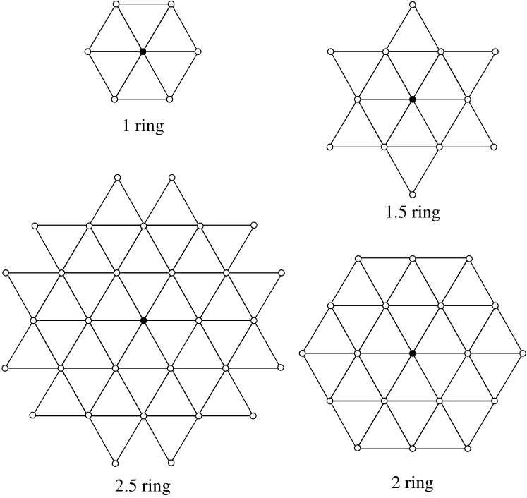
Figure 1: Schematics of 1-ring, 1.5-ring, 2-ring, and 2.5-ring neighbor vertices of center vertex (black) in each illustration.

Observe that a typical $\frac{d+1}{2}$-ring neighborhood has about the ideal number of points for the $d$th degree fittings at least up to degree six, which is evident from Table 1. Therefore, we use this as the general guideline for selecting the points. Note that occasionally (such as for the points near boundary) the $\frac{d+1}{2}$-ring neighborhood may not have enough points. If the number of points is less than $1.5n$, we increase the ring level by $0.5$ up to $3.5$. Note that we do not attempt to filter out the points that are far away from the origin at this stage, because such a filtering is done more systematically through the weighting matrix in (24).

Table 1: Numbers of coefficients in $d$th degree fittings versus numbers of points in typical $\frac{d+1}{2}$ rings.

degree ($d$)	1	2	3	4	5	6
#coeffs.	3	6	10	15	21	28
#points in $\frac{d+1}{2}$ ring	7	13	19	31	37	55

4.3.2 QR Factorization with Safeguard

Our discussions about the point selection was based on a probability argument. Therefore, ill-conditioning may still occur especially near the boundary of a surface mesh. The standard approaches for addressing ill-conditioned rectangular linear systems include SVD or QR factorization with column pivoting (see [Golub and Van Loan 1996, p. 270]. When applied to (27), the former approach would seek a solution that minimizes the 2-norm of the solution vector $\|\mbox{\boldmath$d$}\|_{2}$ among all the feasible solutions, and the latter provides an efficient but less robust approximation to the former. Neither of these approaches seems appropriate in this context, because they do not give higher priorities to the lower derivatives, which are the solutions of interest.

Instead, we propose a safeguard for QR factorization for the local fittings. Let the columns of $V$ (and in turn of $A$) be sorted in increasing order of the derivatives (i.e., in increasing order of $j+k$). Let the reduced QR factorization of $A$$S$ be

$$\mbox{\boldmath$A$}\mbox{\boldmath$S$}=\mbox{\boldmath$Q$}\mbox{\boldmath$R$},$$

where $Q$ is $m\times n$ with orthonormal column vectors and $R$ is an $n\times n$ upper-triangular matrix. The 2-norm condition number of $A$$S$ is the same as that of $R$. To determine whether $A$$S$ is nearly rank deficient, we estimate the condition number of $R$ in 1-norm (instead of 2-norm, for better efficiency), which can be done efficiently for triangular matrices and is readily available in linear algebra libraries (such as DGECON in LAPACK [Anderson et al. 1999]). If the condition number of $R$ is too large (e.g., $\geq 10^{3}$), we decrease the degree of the fitting by removing the last few columns of $A$$S$ that correspond to the highest derivatives. Note that QR factorization need not be recomputed after decreasing the degree of fitting, because it can be obtained by removing the corresponding columns in $Q$ and removing the corresponding rows and columns in $R$. If the condition number is still large, we would further reduce the degree of fitting until the condition number is small or the fitting becomes linear. Let $\tilde{\mbox{\boldmath$Q$}}$ and $\tilde{\mbox{\boldmath$R$}}$ denote the reduced matrices of $Q$ and $R$, and the final solution of $c$ is given by

$$\mbox{\boldmath$c$}=\mbox{\boldmath$S$}\tilde{\mbox{\boldmath$R$}}^{-1}\tilde{\mbox{\boldmath$Q$}}^{T}\mbox{\boldmath$b$},$$ (28)

where $\tilde{\mbox{\boldmath$R$}}^{-1}$ denotes a back substitution step. Compared to SVD or QR with partial pivoting, the above procedure is more accurate for derivative estimation, as it gives higher priorities to lower derivatives, and at the same time it is more efficient than SVD.

4.4 Iterative Fitting of Derivatives

The polynomial fitting above uses only the coordinates of the given points. If accurate normals are known, it can be beneficial to take advantage of them. If the normals are not given a priori, we may estimate them first by using the polynomial fitting described earlier. We refer to this approach as iterative fitting.

First, we convert the vertex normals into the gradients of the height function within the local $uvw$ frame at a point. Let $\hat{\mbox{\boldmath$n$}}_{i}=\left[\alpha_{i},\beta_{i},\gamma_{i}\right]^{T}$ denote the unit normal at the $i$th point in the $uvw$ coordinate system, and then the gradient of the height function is $\left[\begin{array}[]{c}-\alpha_{i}/\gamma_{i}\\ -\beta_{i}/\gamma_{i}\end{array}\right]$. Let $a_{jk}\equiv c_{(j+1)k}$ and $b_{jk}\equiv c_{j(k+1)}$. By plugging $u_{i}$, $v_{i}$, and $f_{u}(u_{i},v_{i})\approx-\alpha_{i}/\gamma_{i}$ into (21), we obtain an equation for the coefficients $a$s; similarly for $f_{v}$ and $b$s. For example, for cubic fittings we obtain the equations

$$a_{00}+a_{10}u_{i}+a_{01}v_{i}+a_{20}\frac{u_{i}^{2}}{2}+a_{11}u_{i}v_{i}+$$

$$a_{02}\frac{v_{i}^{2}}{2}+a_{30}\frac{u_{i}^{3}}{6}+a_{21}\frac{u_{i}^{2}v_{i}}{2}+a_{12}\frac{u_{i}v_{i}^{2}}{2}+a_{03}\frac{v_{i}^{3}}{6} \approx-\frac{\alpha_{i}}{\gamma_{i}},$$ (29)

$$b_{00}+b_{10}u_{i}+b_{01}v_{i}+b_{20}\frac{u_{i}^{2}}{2}+b_{11}u_{i}v_{i}+$$

$$b_{02}\frac{v_{i}^{2}}{2}+b_{30}\frac{u_{i}^{3}}{6}+b_{21}\frac{u_{i}^{2}v_{i}}{2}+b_{12}\frac{u_{i}v_{i}^{2}}{2}+b_{03}\frac{v_{i}^{3}}{6} \approx-\frac{\beta_{i}}{\gamma_{i}}.$$ (30)

If we enforce $a_{j,k+1}=b_{j+1,k}$ explicitly, we would obtain a single linear system for all the $a$s and $b$s with a reduced number of unknowns. Alternatively, $a_{jk}$ and $b_{jk}$ can be solved separately using the same coefficient matrix as (23) and the same weighted least squares formulation, but two different right-hand side vectors, and then $a_{j,k+1}$ and $b_{j+1,k}$ must be averaged. The latter approach compromises the optimality of the solution without compromising the symmetry and the order of convergence. We choose the latter approach for simplicity.

After obtaining the coefficients $a$s and $b$s, we then obtain the Hessian of the height function at $\mbox{\boldmath$u$}_{0}$ as

$$\mbox{\boldmath$H$}_{0}=\left[\begin{array}[]{cc}a_{10}&(a_{01}+b_{10})/2\\ (a_{01}+b_{10})/2&b_{01}\end{array}\right].$$

From the gradient and Hessian, the second-order differential quantities are then obtained using the formulas in Section 3. We summarize the overall iterative fitting algorithm as follows:
1) Obtain initial estimation of vertex normals by averaging face normals for the construction of local coordinate systems at vertices;
2) For each vertex, determine $\frac{d+1}{2}$-ring neighbor vertices and upgrade neighborhood if necessary;
3) For each vertex, transform its neighbor points into its local coordinate frame, solve for the coefficients using QR factorization with safeguard, and convert gradients into vertex normals;
4) If iterative fitting is desired, for each vertex, transform normals of its neighbor vertices to the gradient of the height function in its local coordinate system to solve for Hessian;
5) For each vertex, convert Hessian into symmetric shape operator to compute curvatures, principal directions, or curvature tensor.

In the algorithm, some steps (such as the collection of neighbor points) may be merged into the loops in later steps, with a tradeoff between memory and computation. Note that iterative fitting is optional, because we found it to be beneficial only for odd-degree fittings, as discussed in more detail in the next subsection. Without iterative fitting, the Hessian of the height function should be obtained at step 3. Finally, note that we can also apply the idea of iterative fitting to convert the curvature tensor to the Hessian of the height function and then construct a fitting of the Hessian to obtain higher derivatives. However, since the focus of this paper is on first- and second-order differential quantities, we do not pursue this idea further.

4.5 Error Analysis

To complete the discussion of our framework, we must address the fundamental question of whether the computed differential quantities converge as the mesh gets refined, and if so, what is the convergence rate. While it has been previously shown that polynomial fittings produce accurate normal and curvature estimations in noise-free contexts [Cazals and Pouget 2005, Meek and Walton 2000], our framework is more general and uses different formulas for computing curvatures, so it requires a more general analysis. Let $h$ denote the average edge length of the mesh. We consider the errors in terms of $h$. Our theoretical results have two parts, as summarized by the following two theorems.

Theorem 5.

Given a set of points in $uvw$ coordinate frame that interpolate a smooth height function $f$ or approximate $f$ with an error of $O(h^{d+1})$ along the $w$ direction. Assume the point distribution and the weighing matrix are independent of the mesh resolution, and the scaled matrix $A$$S$ in (27) has a bounded condition number. The degree-$d$ weighted least squares fitting approximates $c_{jk}$ to $O(h^{d-j-k+1})$.

Proof 4.1.

Let $c$ denote the vector composed of $c_{jk}$, the exact partial derivatives of $f$. Let $\tilde{\mbox{\boldmath$b$}}$ denote $A$$c$. Let $\mbox{\boldmath$r$}\equiv\mbox{\boldmath$b$}-\tilde{\mbox{\boldmath$b$}}$, which we consider as a perturbation in the right-hand side of

$$\mbox{\boldmath$A$}\mbox{\boldmath$c$}\approx\tilde{\mbox{\boldmath$b$}}+\mbox{\boldmath$r$}.$$

Because the Taylor polynomial approximates $f$ to $O(h^{d+1})$, and $f$ is approximated to $O(h^{d+1})$ by the given points, each component of $\mbox{\boldmath$f$}-\mbox{\boldmath$V$}\mbox{\boldmath$c$}$ in (23) is $O(h^{d+1})$. Since $\mbox{\boldmath$r$}=\mbox{\boldmath$W$}(\mbox{\boldmath$f$}-\mbox{\boldmath$V$}\mbox{\boldmath$c$})$ and the entries in $W$ are $\Theta(1)$, each component of $r$ is $O(h^{d+1})$.

The error in $c_{jk}$ and in $r$ are connected by the scaled matrix $A$$S$. Since the point distribution are independent of the mesh resolution, $u_{i}=\Theta(h)$ and $v_{i}=\Theta(h)$. The entries in the column of $A$ corresponding to $c_{jk}$ are then $\Theta(h^{j+k})$, so are the $2$-norm of the column. After column scaling, the entries in $A$$S$ are then $\Theta(1)$, so are the entries in its pseudo-inverse $(\mbox{\boldmath$A$}\mbox{\boldmath$S$})^{+}$. The error of $d$ in (27) is then $\delta\mbox{\boldmath$d$}=(\mbox{\boldmath$A$}\mbox{\boldmath$S$})^{+}\mbox{\boldmath$r$}$. Because each component of $r$ is $O(h^{d+1})$, each component of $\delta\mbox{\boldmath$d$}$ is $O(\kappa h^{d+1})$, where $\kappa$ is the condition number of $A$$S$ and is bounded by a constant by assumption. The error in $c$ is then $\mbox{\boldmath$S$}\delta\mbox{\boldmath$d$}$, where the scaling factor associated with $c_{jk}$ is $\Theta(1/h^{j+k})$. Therefore, the coefficient $c_{jk}$ is approximated to $O(h^{d-j-k+1})$.

Note that our weights given in (26) appear to depend on the mesh resolution. However, we can rescale it by multiplying $h^{d/2}$ to make it $\Theta(1)$ without changing the solution, so Theorem 5 applies to our weighting scheme. Under the assumptions of Theorem 5, degree-$d$ fitting approximates the gradient to $O(h^{d})$ and the Hessian to $O(h^{d-1})$ at the origin of the local frame, respectively. Using the gradient and Hessian estimated from our polynomial fitting, the estimated differential quantities have the following property.

Theorem 6.

Given the position, gradient, and Hessian of a height function that are approximated to $O(h^{d+1})$, $O(h^{d})$ and $O(h^{d-1})$, respectively. a) The angle between the computed and exact normals is $O(h^{d})$; b) the components of the shape operator and curvature tensor are approximated $O(h^{d-1})$ by (12) and (13); c) the Gaussian and mean curvatures are approximated to $O(h^{d-1})$ by (16).

Proof 4.2.

a) Let $\tilde{f}_{u}$ and $\tilde{f}_{v}$ denote the estimated derivatives of $f$, which approximate the true derivatives $f_{u}$ and $f_{v}$ to $O(h^{d})$. Let $\tilde{\ell}$ and $\ell$ denote $\|[-\tilde{f}_{u},-\tilde{f}_{v},1]\|$ and $\|[-f_{u},-f_{v},1]\|$, respectively. Let $\tilde{\mbox{\boldmath$n$}}$ denote the computed unit normal $[-\tilde{f}_{u},-\tilde{f}_{v},1]^{T}/\tilde{\ell}$ and $\hat{\mbox{\boldmath$n$}}$ the exact unit normal $[-f_{u},-f_{v},1]^{T}/\ell$. Therefore,

$$\tilde{\mbox{\boldmath$n$}}-\hat{\mbox{\boldmath$n$}}=\frac{\ell[-\tilde{f}_{u},-\tilde{f}_{v},1]^{T}-\tilde{\ell}[-f_{u},-f_{v},1]^{T}}{\ell\tilde{\ell}},$$

where the numerator is $O(h^{d})$ and the denominator is $\Theta(1)$. Let $\theta$ denote $\arccos\tilde{\mbox{\boldmath$n$}}^{T}\hat{\mbox{\boldmath$n$}}$. Because $\|\tilde{\mbox{\boldmath$n$}}-\hat{\mbox{\boldmath$n$}}\|_{2}^{2}=2-2\tilde{\mbox{\boldmath$n$}}^{T}\hat{\mbox{\boldmath$n$}}=\theta^{2}+O(\theta^{4})$, it then follows that $\theta$ is $O(h^{d})$.

b) In (12), if $f_{u}=f_{v}=0$, then $\tilde{\mbox{\boldmath$W$}}=\mbox{\boldmath$H$}$, which is approximated to $O(h^{d-1})$. Otherwise, $H$ is approximated to $O(h^{d-1})$ while $\ell$, $c$, and $s$ are approximated to $O(h^{d})$, so the error in $\tilde{\mbox{\boldmath$W$}}$ is $O(h^{d-1})$. Similarly, in equations (13) and (14), the dominating error term is the $O(h^{d-1})$ error in $H$, while $\mbox{\boldmath$J$}^{+}$ and $\tilde{\mbox{\boldmath$J$}}^{+}$ are approximated to $O(h^{d})$ by their explicit formulas, so $C$ and $\mbox{\boldmath$C$}_{g}$ are approximated to $O(h^{d-1})$.

c) In (16), $\ell$ and $\nabla f$ are approximated to $O(h^{d})$ and $H$ is approximated to $O(h^{d-1})$. Therefore, $\kappa_{G}\$ and $\kappa_{H}$ are both approximated to $O(h^{d-1})$.

The above analysis did not consider iterative fitting. Following the same argument, if the vertex positions and normals are both approximated to $O(h^{d+1)})$ and the scaled coefficient matrix has full rank, then the coefficients $a_{jk}$ and $b_{jk}$ are approximated to order $O(h^{d-j-k+1)})$ by our iterative fitting. The error in the Hessian would then be $O(h^{d})$, so are the estimated curvatures. Therefore, iterative fitting is potentially advantageous, given accurate normals. Note that none of our analyses requires any symmetry of the input data points to achieve convergence. For even-degree fittings, the leading term in the remainder of the Taylor series is odd degree. If the input points are perfectly symmetric, then the residual would also exhibit some degree of symmetry, and the leading-order error term may cancel out as in the centered-finite-difference scheme. Therefore, superconvergence may be expected for even-degree polynomial fittings, and iterative fitting may not be able to further improve their accuracies. Regarding to the principal directions, they are inherently unstable at the points where the maximum and minimum curvatures have similar magnitude. However, if the magnitudes of the principal curvatures are well separated, then the principal directions would also have similar convergence rates as the curvatures.

5 Experimental Results

In this section, we present some experimental results of our framework. We focus on the demonstration of accuracy and stability as well as the advantages of iterative fitting, the weighting scheme, and the safeguarded numerical solver. We do not attempt a thorough comparison with other methods; readers are referred to [Gatzke and Grimm 2006] for such a comparison of earlier methods. We primarily compare our method against the baseline fitting methods in [Cazals and Pouget 2005, Meek and Walton 2000], and assess them for both closed and open surfaces.

5.1 Experiments with Closed Surfaces

We first consider two simple closed surfaces: a sphere with unit radius, and a torus with inner radius $0.7$ and outer radius $1.3$. We generated the meshes using GAMBIT, a commercial software from Fluent Inc. Our focuses here are the convergence rates with and without iterative fitting as well as the effects of the weighting scheme. For convergence test, we generated four meshes for each surface independently of each other by setting the desired edge lengths to $0.1,$ $0.05$, $0.025$, and $0.0125$, respectively. Figure 2 shows two meshes that are coarser but have similar unstructured connectivities as our test meshes.

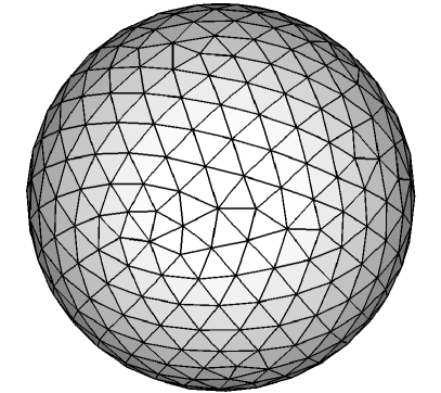
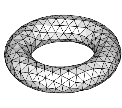
Figure 2: Sample unstructured meshes of sphere and torus.

We first assess the computations of normals using fittings of degrees between one and six. Figure 3 shows the errors in the computed normals versus the “mesh refinement level.” We label the plots by the degrees of fittings. Let $v$ denote the total number of vertices, and let $\hat{\mbox{\boldmath$n$}}_{i}$ and $\tilde{\mbox{\boldmath$n$}}_{i}$ denote the exact and computed unit vertex normals at the $i$th vertex. We measure the relative $L_{2}$ errors in normals as

$$\sqrt{\frac{1}{v}\sum_{1}^{v}\|\tilde{\mbox{\boldmath$n$}}_{i}-\hat{\mbox{\boldmath$n$}}_{i}\|_{2}^{2}}.$$

We compute the convergence rates as

$$\mbox{convergence rate}=\frac{1}{3}\log_{2}\left(\frac{\mbox{error of level 1}}{\mbox{error of level 4}}\right),$$

and show them at the right ends of the curves. In our tests, the convergence rates for normals were equal to or higher than the degrees of fittings. For spheres, the convergence rates of even-degree fittings were about one order higher than predicted, likely due to nearly perfect symmetry and error cancellation.

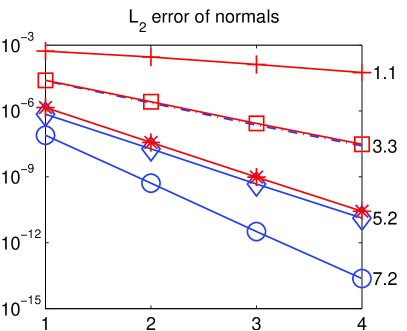
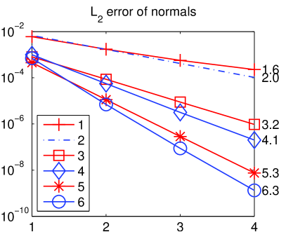
Figure 3: $L_{2}$ errors in computed normals for sphere (left) and torus (right).

Second, we consider the computations of curvatures. It would be excessive to show all the combinations, so we only show some representative results. Figure 4 shows the errors in the minimum and maximum curvatures for the sphere. Figure 5 shows the errors in the mean and Gaussian curvatures for the torus. In the labels, ‘$+$’ indicates the use of iterative fitting. Let $k_{i}$ and $\tilde{k}_{i}$ denote the exact and computed quantities at the $i$th vertex, we measure the relative errors in $L_{2}$ norm as

$$\frac{\|\tilde{\kappa}-\kappa\|_{2}}{\|\kappa\|_{2}}\equiv\left.\sqrt{\sum_{i=1}^{v}\left(\tilde{\kappa}_{i}-\kappa_{i}\right)^{2}}\right/\sqrt{\sum_{i=1}^{v}\kappa_{i}^{2}}.$$ (31)

Let $d$ denote the degree of a fitting. In these tests, the convergence rates were $d-1$ or higher as predicted by theory. In addition, even-degree fittings converged up to one order faster due to error cancellation. The converge rates for odd-degree polynomials were about $d-1$ but were also boosted to approximately $d$ when iterative fitting is used. Therefore, iterative fitting is effective in improving odd-degree fittings. In our experiments, iterative fitting did not improve even-degree fittings.

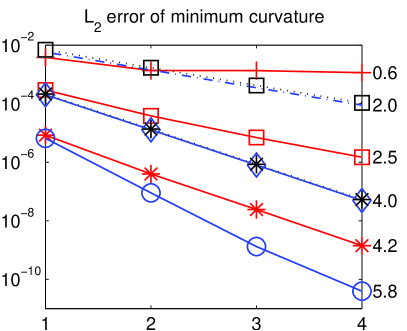
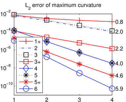
Figure 4: $L_{2}$ errors in computed minimum and maximum curvatures for sphere.

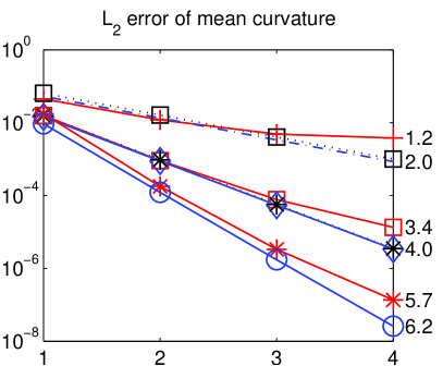
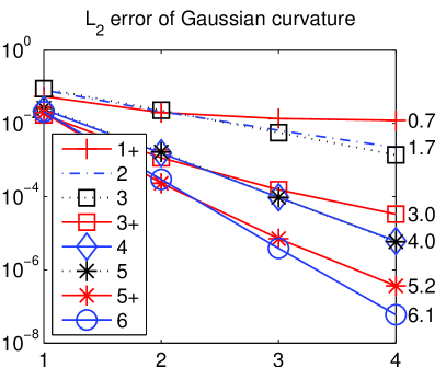
Figure 5: $L_{2}$ errors in computed mean and Gaussian curvatures for torus.

The preceding computations used the weighting scheme described in Section 4.1, which tries to balance conditioning and error cancellation. This weighting scheme improved the results in virtually all of our tests. Figure 6 shows a representative comparison with and without weighting (as labeled by “$\cdot$nw” and “$\cdot$w”, respectively) for the maximum curvatures of the sphere and torus.

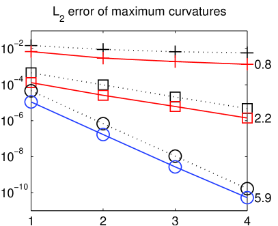
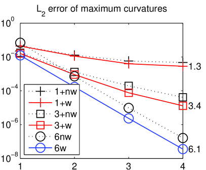
Figure 6: Comparisons of curvature computations with and without weighting for sphere (left) and torus (right).

5.2 Experiments with Open Surfaces

We now consider open surfaces, i.e. surfaces with boundary. We focus on the study of stabilities and the effects of boundary and irregular connectivities. We use two surfaces defined by the following functions adopted from [Xu 2004]:

$$z=F_{1}(x,y)= \frac{1.25+\cos(5.4y)}{6+6(3x-1)^{2}},$$ (32)

$$z=F_{2}(x,y)= \exp\left(-\frac{81}{16}\left((x-0.5)^{2}+(y-0.5)^{2}\right)\right),$$ (33)

where $(x,y)\in[0,1]\times[0,1]$. Figure 7(a-b) shows these surfaces, color-coded by the mean curvatures. We use two types of meshes, including irregular and semi-regular meshes (see Figure 7(c-d)). For convergence study, we refine the irregular meshes using the standard one-to-four subdivision [Gallier 2000, p. 283] and refine the semi-regular meshes by replicating the pattern. We computed the “exact” differential quantities using the formulas in Section 3 in the global coordinate system, but performed all other computations in local coordinate systems. For rigorousness of the tests, we consider both $L_{2}$ and $L_{\infty}$ errors. In addition, border vertices are included in all the error measures, posting additional challenges to the tests. Note that the results for vertices far away from the boundary would be qualitatively similar to those of closed surfaces. We primarily consider fittings of up to degree four, since higher convergence rates may require larger neighborhoods for border vertices (more than $3.5$-ring neighbors). To limit the length of presentation, we report only some representative results to cover the aforementioned different aspects.

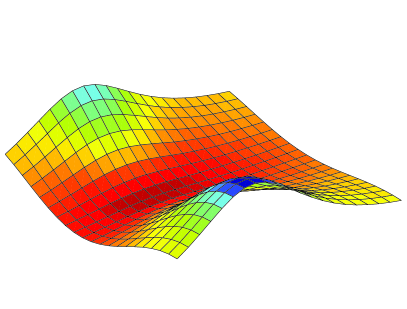
(a) $F_{1}$.

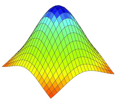
(b) $F_{2}$.

(c) Irregular mesh.

(d) Semi-regular mesh.

Figure 7: Test surfaces (a-b) and meshes (c-d). Surfaces are color-coded by mean curvatures.

We first assess the errors in the computed normals for open surfaces. Figure 8 shows the results for $F_{1}$ over irregular meshes. We label all the plots and convergence rates in the same way as for closed surfaces. Let $d$ denote the degree of a fitting. All these fittings delivered convergence rate of $d$ or higher in $L_{2}$ errors. In $L_{\infty}$ errors, computed as $\max_{i}\|\tilde{\mbox{\boldmath$n$}}_{i}-\hat{\mbox{\boldmath$n$}}_{i}\|_{2}$, the convergence rates were $d-0.5$ or higher, close to theoretical predictions.

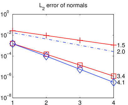
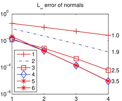
Figure 8: $L_{2}$ (left) and $L_{\infty}$ (right) errors in computed normals for $F_{1}$ over irregular meshes.

Second, we assess the errors in the curvatures. Figure 9 shows the errors in mean curvatures for $F_{1}$ over irregular meshes, and Figure 10 shows the errors in Gaussian curvatures for $F_{2}$ over semi-regular meshes. Let $\kappa$ and $\tilde{\kappa}$ denote the exact and computed quantities. We computed the $L_{2}$ error using (31) and computed the $L_{\infty}$ errors as

$$\max_{i}\left|\tilde{\kappa}_{i}-\kappa_{i}\right|/\max\{\left|\kappa_{i}\right|,\epsilon\},$$ (34)

where $\epsilon=0.01\max_{i}\left|\kappa_{i}\right|$ was introduced to avoid division by too small numbers. The convergence rates for curvatures were approximately equal to $d-1$ or higher for even-degree fittings and odd-degree iterative fittings.

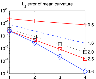
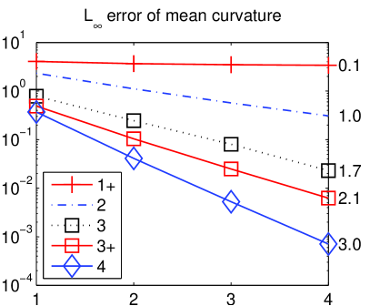
Figure 9: $L_{2}$ (left) and $L_{\infty}$ (right) in computed mean curvatures for $F_{1}$ over irregular meshes.

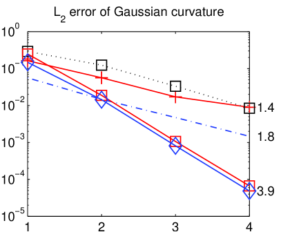
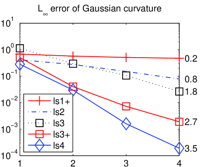
Figure 10: $L_{2}$ (left) and $L_{\infty}$ (right) in computed Gaussian curvatures for $F_{2}$ over semi-regular meshes.

As noted earlier, the principal directions are inherently unstable when the principal curvatures are roughly equal to each other (such as at umbilic points). In Figure 11, we show the $L_{2}$ and $L_{\infty}$ errors of principal directions for $F_{1}$ over semi-regular meshes, where the errors are measured similarly as for normals. This surface is free of umbilic points, and the principal directions converged at comparable rates as curvatures for iterative cubic fitting and quartic fitting.

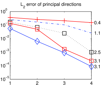
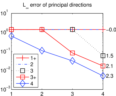
Figure 11: $L_{2}$ (left) and $L_{\infty}$ (right) in computed principal directions for $F_{1}$ over semi-regular meshes.

Finally, to demonstrate the importance and effectiveness of our conditioning procedure, Figure 12 shows comparison of computed normals and mean curvatures with and without conditioning (as labeled by “$\cdot$nc” and “$\cdot$c”, respectively) for fittings of degrees three, five, and six. Here, the conditioning refers to requiring number of points to be $1.5$ or more times of the number of unknowns as well as the checking of condition numbers. Without conditioning, the results exhibited large errors for normals and catastrophic failures for curvatures, due to numerical instabilities. With conditioning, our framework is stable for all the tests, although it did not achieve the optimal convergence rate for the sixth-degree fittings due to too small neighborhoods for the vertices near boundary.

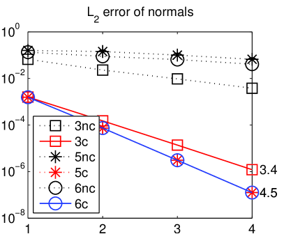
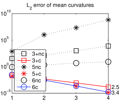
Figure 12: Comparisons of errors in computed normals (left) and mean curvatures (right) with and without conditioning for $F_{1}$ over irregular meshes.

6 Discussions

In this paper, we presented a computational framework for computing the first- and second-order differential quantities of a surface mesh. This framework is based on the computation of the first- and second-order derivatives of a height function, which are then transformed into differential quantities of a surface in a simple and consistent manner. We proposed an iterative fitting method to compute the derivatives of the height function starting from the points with or without the surface normals, solved by weighted least squares approximations. We improve the numerical stability by a systematic point-selection strategy and QR factorization with safeguard. By achieving both accuracy and stability, our method delivered converging estimations of the derivatives of the height function and in turn the differential quantities of the surfaces.

The main focus of this paper has been on the consistent and converging computations of differential quantities. We did not address the robustness issues for input surface meshes with large noise and singularities (such as sharp ridges and corners). We have conducted some preliminary comparisons with other methods, which we will report elsewhere. One of the major motivating application of this work is provably accurate and stable solutions of geometric flows for geometric modeling and physics-based simulations. We are currently investigating the stability of our proposed methods for such problems. Another future direction is to generalize our method to compute higher-order differential quantities.

References

- [\citenameAgam and Tang 2005] Agam, G., and Tang, X. 2005. A sampling framework for accurate curvature estimation in discrete surfaces. IEEE Trans. Vis. Comput. Graph. 11, 573–583.
- [\citenameAnderson et al. 1999] Anderson, E., Bai, Z., Bischof, C., Blackford, S., Demmel, J., Dongarra, J., Du Croz, J., Greenbaum, A., Hammarling, S., McKenney, A., and Sorensen, D. 1999. LAPACK User’s Guide, 3rd ed. SIAM.
- [\citenameCazals and Pouget 2005] Cazals, F., and Pouget, M. 2005. Estimating differential quantities using polynomial fitting of osculating jets. Comput. Aid. Geom. Des. 22, 121–146.
- [\citenameCohen-Steiner and Morvan 2003] Cohen-Steiner, D., and Morvan, J.-M. 2003. Restricted Delaunay triangulations and normal cycle. In Proc. of 19th Annual Symposium on Computational Geometry, 312–321.
- [\citenamede Boor and Ron 1992] de Boor, C., and Ron, A. 1992. Computational aspects of polynomial interpolation in several variables. Math. Comp. 58, 705–727.
- [\citenamedo Carmo 1976] do Carmo, M. P. 1976. Differential Geometry of Curves and Surfaces. Prentice-Hall.
- [\citenamedo Carmo 1992] do Carmo, M. P. 1992. Riemannian Geometry. Birkhäuser Boston.
- [\citenameGallier 2000] Gallier, J. 2000. Curves and Surfaces in Geometric Modeling: Theory and Algorithms. Morgan Kaufmann.
- [\citenameGatzke and Grimm 2006] Gatzke, T., and Grimm, C. 2006. Estimating curvature on triangular meshes. Int. J. Shape Modeling 12, 1–29.
- [\citenameGoldfeather and Interrante 2004] Goldfeather, J., and Interrante, V. 2004. A novel cubic-order algorithm for approximating principal direction vectors. ACM Trans. Graph. 23, 45–63.
- [\citenameGolub and Van Loan 1996] Golub, G. H., and Van Loan, C. F. 1996. Matrix Computation, 3rd ed. Johns Hopkins.
- [\citenameGrinspun et al. 2006] Grinspun, E., Gingold, Y., Reisman, J., and Zorin, D. 2006. Computing discrete shape operators on general meshes. Eurographics (Computer Graphics Forum) 25, 547–556.
- [\citenameHildebrandt et al. 2006] Hildebrandt, K., Polthier, K., and Wardetzky, M. 2006. On the convergence of metric and geometric properties of polyhedral surfaces. Geometria Dedicata 123, 89–112.
- [\citenameLancaster and Salkauskas 1986] Lancaster, P., and Salkauskas, K. 1986. Curve and Surface Fitting: An Introduction. Academic Press.
- [\citenameLanger et al. 2005a] Langer, T., Belyaev, A. G., and Seidel, H.-P. 2005. Analysis and design of discrete normals and curvatures. Tech. rep., Max-Planck-Institut Für Informatik.
- [\citenameLanger et al. 2005b] Langer, T., Belyaev, A. G., and Seidel, H.-P. 2005. Exact and approximate quadratures for curvature tensor estimation. In Poster Proc. of Symposium on Geometry Processing.
- [\citenameMeek and Walton 2000] Meek, D. S., and Walton, D. J. 2000. On surface normal and Gaussian curvature approximations given data sampled from a smooth surface. Comput. Aid. Geom. Des. 17, 521–543.
- [\citenameMeyer et al. 2002] Meyer, M., Desbrun, M., Schröder, P., and Barr, A. 2002. Discrete differential geometry operators for triangulated 2-manifolds. In Visualization and Mathematics, H.-C. Hege and K. Poltheir, Eds., vol. 3. Springer, 34–57.
- [\citenameOhtake et al. 2004] Ohtake, Y., Belyaev, A., and Seidel, H.-P. 2004. Ridge-valley lines on meshes via implicit surface fitting. ACM Trans. Graph. 23, 609–612.
- [\citenameOńate and Cervera 1993] Ońate, E., and Cervera, M. 1993. Derivation of thin plate bending elements with one degree of freedom per node. Engineering Computations 10, 543.
- [\citenamePetitjean 2002] Petitjean, S. 2002. A survey of methods for recovering quadrics in triangle meshes. ACM Comput. Surveys 34, 211–262.
- [\citenamePinkall and Polthier 1993] Pinkall, U., and Polthier, K. 1993. Computing discrete minimal surfaces and their conjugates. Exper. Math. 2, 15–36.
- [\citenameRazdan and Bae 2005] Razdan, A., and Bae, M. 2005. Curvature estimation scheme for triangle meshes using biquadratic Bézier patches. Comput. Aid. Des. 37, 1481–1491.
- [\citenameRusinkiewicz 2004] Rusinkiewicz, S. 2004. Estimating curvatures and their derivatives on triangle meshes. In Proc. of 2nd International Symposium on 3D Data Processing, Visualization and Transmission, 486–493.
- [\citenameTaubin 1995] Taubin, G. 1995. Estimating the tensor of curvature of a surface from a polyhedral approximation. In Proc. of Int. Conf. on Computer Vision, 902–907.
- [\citenameTheisel et al. 2004] Theisel, H., Rossl, C., Zayer, R., and Seidel, H.-P. 2004. Normal based estimation of the curvature tensor for triangular meshes. In 12th Pacific Conf. on Computer Graphics and Applications, 288–297.
- [\citenamevan der Sluis 1969] van der Sluis, A. 1969. Condition numbers and equilibration of matrices. Numer. Math. 14, 14–23.
- [\citenameWardetzky 2007] Wardetzky, M. 2007. Convergence of the cotan formula - an overview. In Discrete Differential Geometry, A. I. Bobenko, J. M. Sullivan, P. Schröder, and G. Ziegler, Eds. Birkhäuser Basel.
- [\citenameXu 2004] Xu, G. 2004. Convergence of discrete Laplace-Beltrami operators over surfaces. Comput. Math. Appl. 48, 347–360.
- [\citenameYang et al. 2006] Yang, Y.-L., Lai, Y.-K., Hu, S.-M., and Pottmann, H. 2006. Robust principal curvatures on multiple scales. In Eurographics Symposium on Geometry Processing.
- [\citenameZorin 2005] Zorin, D. 2005. Curvature-based energy for simulation and variational modeling. In Int. Conf. on Shape Modeling and Applications, 196–204.