Phase Separation under Ultra-Slow Cooling: Onset of Nucleation

Abstract

We discuss the interplay between a slow continuous drift of temperature, which induces continuous phase separation, and the non-linear diffusion term in the $\phi^{4}$-model for phase separation of a binary mixture. This leads to a bound for the stability of diffusive demixing. It is argued that these findings are not specific to the $\phi^{4}$ model, but that they always apply up to slight modifications of the bound. In practice stable diffusive demixing can only be achieved when special precautions are taken in experiments on real mixtures. Therefore, the recent observations on complex dynamical behavior in such systems should be considered as a new challenge for understanding generic features of phase-separating systems.

I Introduction

The kinetics of phase separation Lifshitz and Slyozov (1961); Siggia (1979); Gunton et al. (1983); Bray (1994); Binder (1998); Onuki (2002) is a topic of continuous experimental Tanaka (1994); Tanaka and Sighuzi (1995); Vollmer et al. (1997a, b, c); Vollmer and Vollmer (1999) and theoretical interest Wagner and Yeomans (1998); Kendon et al. (1999); Puri and Binder (2001). Many of its characteristic features do not depend on specific materials, but are universal in the sense that they can be understood based on relatively simple model systems. For binary mixtures an appropriate model is the $\phi^{4}$ model Bray (1994); Binder (1998); Chaikin and Lubensky (2000). In the present paper we augment this model by terms taking into account a slow continuous drift of the temperature, in order to explore how the composition of coexisting phases keeps up with the driving due to the temperature evolution.

Typically the demixing dynamics of binary fluids is idealized as a three step process:
A.  A rapid change of the temperature (pressure or other experimental control parameter) transfers the system from a single phase equilibrium into the region, where phase separation is expected [cooling in Fig. 1]. This is supposed to be sufficiently fast to neglect noticeable changes in the composition.
B.  The mixture decomposes into two coexisting macroscopic phases [decomposition in Fig. 1]. In applications this is supposed to be fast on the time scales of changing the temperature; in high precision experiments Wong and Knobler (1981); Chou and Goldburg (1981); Joshua and Goldburg (1985); Tanaka (1994); Tanaka and Sighuzi (1995); Cumming et al. (1990) a temperature jump is applied and the temperature is subsequentially fixed to carefully observe the dynamics in this regime.
C.  Upon further slow cooling there is an exchange of material such that the composition of the coexisting phases follows the equilibrium ones up to a small time lag [smooth green line denoted segregation in Fig. 1].

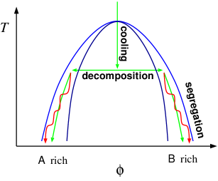
Figure 1: (Color online) Schematic phase diagram for the demixing of a binary mixture. The binodal is given in blue and the spinodal line in dark blue. A typical evolution of the composition $\phi$ of the mixture upon constant cooling is indicated by the green line. The red line shows an oscillating demixing, as it may be observed when the diffusive decomposition becomes unstable.

A dimensional analysis of the diffusive relaxation time Cates et al. (2003); Auernhammer et al. (2005); Vollmer et al. (2007) shows, however, that for experimentally relevant cooling rates the composition can not remain close to the equilibrium values unless temperature is ramped exceedingly slowly. Indeed, recent experimental Sparks et al. (1993); Vollmer et al. (1997a, b); Vollmer and Vollmer (1999); Vollmer et al. (1997c); Heimburg et al. (2000); Vollmer et al. (2002); Turchanin and Freyland (2004); Turchanin et al. (2004); Auernhammer et al. (2005) and numerical studies Wagner et al. (2003); Cates et al. (2003) indicate that rather than slowly following the drift of the equilibrium composition, often there is very complex dynamics observed in regime C. Among others secondary nucleation in large domains (double phase separation) Tanaka and Sighuzi (1995), oscillating bursts of massive phase separation alternating with quiescent periods Vollmer et al. (1997a, b); Vollmer and Vollmer (1999); Vollmer et al. (1997c); Heimburg et al. (2000); Vollmer et al. (2002); Turchanin and Freyland (2004); Turchanin et al. (2004) and stationary convection patterns Cates et al. (2003) have been reported. Except for the stationary convection, all these scenarios give rise to an explicitly time dependence of the composition like the one indicated by the red line in Fig. 1.

Despite the impressive experimental findings, the theoretical understanding of such complex dynamical response to slow cooling is still at its infancy. To make a point, however, on the prevalence of the various complex patterns of phase separation the present paper explores the critical cooling rate beyond which stable diffusive demixing can no longer be expected.

The article is organized as follows. Section Sec. II revisits the relevant nonlinear diffusion equation describing the evolution of concentration in a slowly cooled binary mixture. In Sec. III we consider the limit of a very narrow interface at the meniscus in order to analytically derive a phase portrait which gives us access to discuss stable and unstable solutions of the diffusion equation, and their bifurcations. A generalization of this discussion to the case where the phases are not symmetric is given in App. A. The subsequent Sec. IV introduces a mode expansion in order to gain insight in the time evolution of the profiles after bifurcations, and the role of higher order derivatives needed to properly describe interfaces of finite thickness. (Technical issues of its derivation have been delegated to App. B.) The main results are summarized in Sec. V.

            

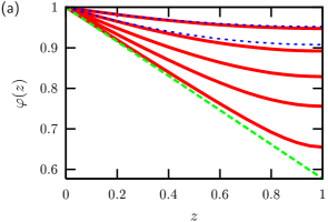
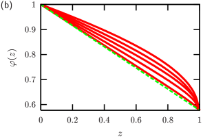
Figure 2: (Color online) Stationary density profiles for $M=0$ and $N=0.1,0.2,0.3,0.4,0.50$ (solid red lines from top to bottom), and the critical parameter $N_{c}=(\sqrt{3}-1)^{2}\simeq 0.5359$ (dashed green curve): (a) stable solutions with $\varphi^{\prime}(z=1)=0$; (b) unstable solutions, which all end at $\varphi_{s}=3^{-1/2}\simeq 0.58$. The dotted blue lines in part (a) show the approximation (10) for $N=0.1$ and $N=0.2$, respectively.

II Nonlinear Diffusion Equation

We describe the temporal evolution of the binary mixture by the free energy functional Chaikin and Lubensky (2000)

$${\mathcal{F}}[\phi(\mathbf{x};t),t]=\int{\mathrm{d}}\mathbf{x}\left[F_{0}[\phi(\mathbf{x};t)]+\frac{K}{2}\>\left(\nabla\phi(\mathbf{x};t)\right)^{2}\right]$$ (1)

where $\phi(x)$ characterizes the composition at position $x$, and the integration over $\mathbf{x}$ is performed over the volume of the system. The second term in square brackets represents an energy penalty for steep changes of composition (macroscopically it gives rise to surface tension), and

$$F_{0}(\phi) \equiv \frac{B}{4}\phi^{4}+\frac{A}{2}\phi^{2}$$ (2)

$$= -A\phi_{0}^{2}\left[\frac{1}{4}\left(\frac{\phi}{\phi_{0}}\right)^{4}-\frac{1}{2}\left(\frac{\phi}{\phi_{0}}\right)^{2}\right]$$

is the free energy of the $\phi^{4}$-model, which describes the equilibrium phase behavior of the mixtures. In the present study we only deal with negative values of $A$, where there are two coexisting phases with composition $\pm\phi_{0}$ and $\phi_{0}\equiv\sqrt{-A/B}$. The temperature dependence of the equilibrium composition $\phi_{0}(T)$ is due to the temperature dependence of the parameters $A$ and $B$.

The free energy (2) faithfully accounts for qualitative features of the demixing of fluid mixtures, even though more complicated expressions may arise for concrete systems Bray (1994); Chaikin and Lubensky (2000). The explicit time dependence in Eq. (1) accounts for the fact that we deal with a system subjected to a sustained change of temperature. Due to its temperature dependence the equilibrium composition $\phi_{0}$ becomes explicitly time dependent in that case.

In the absence of center of mass flow the interdiffusion of the components of the mixtures follows

$$\partial_{t}\phi(\mathbf{x};t)=\alpha\nabla^{2}\mu[\phi(\mathbf{x};t)]$$

where $\alpha$ is the thermodynamic coefficient for mass interdiffusion, and the chemical potential $\mu[\phi]\equiv\delta(F_{0}[\phi]+K/2\,[\nabla\phi]^{2})/\delta\phi$ is the functional derivative of the free energy density (1) with respect to $\phi$. Consequently, the normalized composition $\varphi\equiv\phi/\phi_{0}$ evolves according to the nonlinear diffusion equation

$$\partial_{t}\varphi=\nabla\left[\frac{D}{2}\left(3\varphi^{2}-1\right)\>\nabla\varphi\right]-D\delta^{2}\,\nabla^{4}\varphi-\xi\,\varphi$$ (3)

where

$$\xi\equiv\frac{\partial_{t}\phi_{0}}{\phi_{0}}$$ (4)

accounts for the change of the equilibrium composition due to the changing temperature, $\delta\equiv(K/|A|)^{1/2}$ is the width of a planar macroscopic interface between the coexisting phases Chaikin and Lubensky (2000), and $D\equiv-\alpha A$ is the equilibrium diffusion coefficient (i. e., the one for a system with uniform composition $\varphi\equiv\pm 1$). Away from equilibrium the diffusion becomes nonlinear with a diffusion coefficient $D\,(3\varphi^{2}-1)/2$ explicitly depending on composition. In the spinodal range $-\varphi_{s}\equiv-1/\sqrt{3}<\varphi<1/\sqrt{3}\equiv\varphi_{s}$ the diffusion coefficient even takes negative values, indicating the instability of the mixture against arbitrarily small fluctuations.

In the following we focus on the simplest setting allowing us to discuss the breakdown of diffusion — generalizations are outlined in App. A:
(i) There are equal amounts of the components A and B of the mixture such that in equilibrium there is a macroscopic A-rich phase coexisting with a B-rich one.
(ii) The mixture is kept in a container of constant cross section and height $2\Lambda$, and it is subjected to a gravitational field. As a consequence there is a macroscopic phase boundary at $z=0$. The bottom and top walls of the container are at $z=\pm\Lambda$, respectively.
(iii) The flux through the bottom and top of the system vanishes.
(iv) There is no flow in the horizontal directions such that $\partial_{x}\varphi=\partial_{y}\varphi=0$.
(v) The temperature is changed in such a way that $\xi$ is constant (cf. Auernhammer et al. (2005)).
(vi) The temperature and composition dependence of the equilibrium diffusion coefficient $D$ may be neglected.

Spacial scales are conveniently measured in units of $\Lambda$, and time in units of $\Lambda^{2}/D$. The resulting dimensionless diffusion equation

$$\partial_{t}\varphi=\partial_{z}\left[\frac{3\varphi^{2}-1}{2}\>\partial_{z}\varphi\right]-M^{2}\>\partial_{z}^{4}\varphi-N\>\varphi$$ (5)

takes a universal form for all the mixtures. It only involves the dimensionless parameters

$$N \equiv \frac{\xi\Lambda^{2}}{D},$$ (6a)

$$M \equiv \frac{\delta}{\Lambda}.$$ (6b)

The former characterized the strength of the driving by the ratio of the rate of generation $\xi$ of supersaturation over the rate of decay of supersaturation due to diffusion. The latter characterizes the importance of the boundary layer at the meniscus between the coexisting phases by the ratio of the interface width $\delta$ over the system size $\Lambda$.

Equation (5) ought to be solved subject to no-flux boundary conditions (iii) at the top and bottom of the system, viz.

$$0=\left[\,\frac{3\varphi^{2}-1}{2}\>\partial_{z}\varphi-M\>\partial_{z}^{3}\varphi\,\right]_{z=\pm 1}.$$ (7)

To ensure mass overall conservation we furthermore demand $\varphi(z)=-\varphi(z)$ .

III Stationary diffusion profiles

Except in the critical region (i. e., the region very close to the maximum of the coexistence curve in Fig. 1) the width $\delta$ of the interface is always much smaller than the lateral extension $\Lambda$ of a macroscopic system. Observing that a temperature ramp rapidly moves the mixture out of this region, one may assume $M\equiv\delta/\Lambda\ll 1$ in systems of macroscopic dimension $\Lambda$. Consequently, the term with the fourth order derivative, which accounts for the effects of surface tension, is only relevant in situations where there are very rapid changes of composition. This only is the case close to $z=0$ at the interface between the coexisting phases, and for values of $\varphi$ close to the threshold of spinodal decomposition (cf. below). Typically it has only negligible influence on the supersaturation profile $\varphi(z;t)$. To gain insight in its dependence on $N$ we therefore discuss the $\varphi(z)$ profiles in the idealized case $M=0$, where the diffusion equation

$$\partial_{t}\varphi=\partial_{z}\left[\frac{3\varphi^{2}-1}{2}\>\partial_{z}\varphi\right]-N\>\varphi$$ (8)

will be subjected to the boundary conditions

$$z=0^{\pm}: \qquad\qquad\qquad\varphi(z=0)=\pm 1,$$ (9a)

$$z=\pm 1: \frac{3\varphi^{2}-1}{2}\>\partial_{z}\varphi(z=\pm 1;t)=0.$$ (9b)

The former requires that the the composition takes on the equilibrium value at the meniscus, and the latter that there is no flux through the top and bottom interfaces of the system. There are two possibilities to fulfill the latter boundary condition (Fig. 2):
(a) stable diffusion profiles are obtained for $\partial_{z}\varphi(z=\pm 1)=0$;
(b) when the composition at the top and/or bottom of the system exactly amounts to the spinodal composition $\varphi(z=\pm 1)=\varphi_{s}=3^{-1/2}$ the factor in front of the derivative vanishes, and one obtains an unstable diffusion profile.
These possibilities will be further explored in the remainder of this section. The question in how far the findings based on this idealized setting still apply at a non-vanishing $M$ will be addressed in Sec. IV.

III.1 Stable diffusion profiles

For very weak driving, $N\lll 1$, the composition $\varphi$ never substantially differs from its equilibrium value, such that $(3\varphi^{2}-1)/2\simeq 1$. In other words the diffusion coefficient hardly depends on $\varphi$, such that it may be approximated by its equilibrium value. In this case the boundary condition (7) at the top requires $\partial_{z}\varphi=0$, and one easily checks that the stationary solution of the diffusion equation amounts to

$$\varphi(z)=\frac{\cosh\left[\sqrt{N}\;(z-1)\right]}{\cosh\left[\sqrt{N}\right]}.$$ (10)

For $N=0.1$ and $N=0.2$ it is shown by a dotted blue line in Fig. 2(a). Indeed the approximation appears to be very good as long as $N\lesssim 0.1$.

For larger values of $N$ the $\varphi$-profile deviates too strongly from unity to neglect the supersaturation dependence of the diffusion coefficient. In that case the solution of the diffusion equation (5) can not be given in a closed form. Upon numerical integration one observes, however, that close to $z=0$ it closer and closer approaches the linear solution

$$\varphi(z)=1-\sqrt{\frac{N}{3}}\;z.$$ (11)

Unless $N=N_{c}\equiv(\sqrt{3}-1)^{2}\simeq 0.5359$ this linear solution does not fulfill the no-flux boundary condition (9b) at the surface $z=0$. Consequently, the solution eventually crosses over into an approximately parabolic profile with a minimum at $z=1$ (solid red lines in Fig. 2(a)). In the limit $N\to N_{c}$ the stable solutions closer and closer approaches the linear solution $1-\sqrt{N_{c}/3}\,x$, which for $N=N_{c}$ fulfills the boundary condition (7) because the ratio preceding $\partial_{z}\varphi$ vanishes.

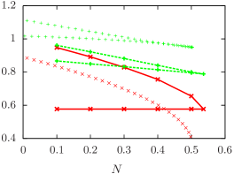
Figure 3: (Color online) The values $\varphi(z=1/2)$ (thick green $+$ connected by dahsed lines) and $\varphi(z=1)$ (thick red $\times$ connected by solid lines) of the stable (upper curve) and unstable (lower curve) solution as a function of the dimensionless ramp rate $N$. The respective approximations by the two mode model Eq. (18) are indicated by corresponding small symbols.

The corresponding small symbols show

III.2 Unstable stationary profiles and a saddle-node bifurcation

From a physical point of view the linear solution for $N_{c}$ has no flux across the top surface since the nonlinear diffusion coefficient $(3\varphi^{2}-1)D/2$ vanishes at the spinodal. There are several observation to be made about this solution:
(i) Since the composition close to the top of the system approaches the value at the spinodal line, the linear profile is unstable against nucleation of domains of the minority phase close to top end. As a consequence the stable solutions of the diffusion equation approach an unstable solution, when $N\to N_{c}$.
(ii) Besides being the limiting behavior of the stable solutions, the linear profile can also be viewed as a limiting case of a family of solutions that end on the spinodal point at the top of the system (solid red lines in Fig. 2(b)). All these solutions are unstable against nucleation of domains of the minority phase close to top end.
(iii) At the critical parameter value $N_{c}$ the family of stable solutions of the diffusion equation collides with the unstable ones in a saddle node bifurcation. Subsequently, there is no stationary diffusive solution with only two domains in the vertical direction. In order to clearly make this point Fig. 3 shows the values $\varphi(z=1/2)$ and $\varphi(z=1)$ for the coexisting stable (upper curves) and unstable (lower curves) solutions.

This result still holds for non-vanishing $M$, since $\partial_{z}^{4}\varphi$ vanishes for a linear profile. Moreover, it also does not rely on the specific dependence $(3\varphi^{2}-1)/2$ of the $\phi^{4}$ model. When the supersaturation dependence of the diffusion is an even 2nd order polynomial $(a\varphi^{2}-b)/(a-b)$ the stable and unstable profiles still approach a linear profile which approaches the spinodal concentration $\varphi_{s}=\sqrt{a/b}$ exactly at the critical point

$$N_{c}=2\;\frac{1-\varphi_{s}}{1+\varphi_{s}}$$ (12)

where the stable and the unstable profile merge and disappear in a saddle node bifurcation. The representation of the stationary profiles via flow diagrams provides us with more insight into the structure of the solutions, and how they might change upon changes of the transport process.

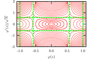
Figure 4: (Color online) Flow diagram of Eq. (8) with $M=0$ and $N$ absorbed in the length scale (cf. text). The equilibrium ($\varphi=\pm 1$) and spinodal ($\varphi=\pm 1/\sqrt{3}$) compositions are marked by vertical dashed green lines. Note that the linear profiles (11) run horizontally on lines $\varphi^{\prime}/\sqrt{N}=\pm 1/\sqrt{3}$, which are also indicated by dashed green lines.

III.3 Flow diagram

The different types of stationary supersaturation profiles $\varphi(z)$ can conveniently be summarized by observing that in Eq. (8) the control parameter $N=\xi\Lambda^{2}/D$ can be absorbed into the length scale, for instance by choosing $z\to\hat{z}\equiv z/\sqrt{N}=(D/\xi)^{1/2}\,z/\Lambda$ . The equation (8) has no free parameter in that case, such that each choice of initial conditions $(\varphi(1);\varphi^{\prime}(1))$ leads to a unique stationary solution of the diffusion equation. In other words, the solutions of Eq. (8) at different $N$ only differ by a rescaling of the length scale. Consequently, all solutions can be represented as a flow diagram in the $(\varphi,\varphi^{\prime}/\sqrt{N})$ plane (Fig. 4).

The flow is symmetric with respect to reflections at both coordinate axes. The symmetry with respect to reflections at the horizontal axis reflects the free choice of the orientation of the $z$ axis. The inversion symmetry of the plot is a consequence of the symmetry between the phases in the $\phi^{4}$ model. In Eq. (8) these symmetries amount to invariance under $z\to-z$ and $\varphi\to-\varphi$. The symmetries are a consequence of the assumption that there are equal amounts of A and B in the mixture, and that the free energy is symmetric with respect to interchanging A and B. App. A demonstrates that our findings do not substantially change in the non-symmetric case. There are only changes of unstable trajectories residing entirely in the spinodal regime where $|\varphi|<\varphi_{s}$. Up to this change the flow is structurally stable (cf. Arnold (2008)) upon variation of the functional form of the source term (as long as it remains continuous and strictly monotonous) and the dependence of the diffusion on the supersaturation (as long as one replaces $(3\varphi-1)/2$ by a continuous convex function which takes the value unity at the equilibrium compositions $\varphi=\pm 1$ and negative values somewhere in between).

In order to identify the trajectories in Fig. 4 with the profiles shown in Fig. 2, we observe that all solutions shown in Fig. 2 have in common that $z_{0}=0$ and $\varphi(0)=1$. They differ in the choice of the initial slope $\varphi^{\prime}(0)/\sqrt{N}$. There is a stable solution with slope $\varphi^{\prime}(1)$ slightly smaller than $\sqrt{N/3}$, and an unstable solution where the slope is initially somewhat larger. For stronger driving the initial slopes of the solutions ever closer approach $\sqrt{N/3}$, and the solutions remain linear for longer times.

In the phase flow the profiles all correspond to trajectories which start on the line $\varphi=1$ (rightmost dashed green line) and move inward with a negative initial slope. If $0\geq\varphi^{\prime}(0)/\sqrt{N}>-1/\sqrt{3}$ one obtains a stable profile, which ends on the line $\varphi^{\prime}=0$. For $\varphi^{\prime}(0)<-1/\sqrt{3}$ one obtains an unstable profile, which terminates with infinite slope at the vertical green line $\varphi=1/\sqrt{3}$, which indicates the spinodal $\varphi_{s}$. For each choice of $N$ there is exactly one stable trajectory and one unstable trajectory, which fulfill these boundary conditions for $z=1$. In addition there are symmetry-related solutions in the four other quadrants of the diagram.

In addition to the supersaturation profiles, which start at $\varphi=1$ there are additional stationary states where the supersaturation always lies within the spinodal regime. More complicated profiles can be build by concatenation of pieces of profiles, provided that $(3\varphi^{2}-1)\,\varphi^{\prime}(z)$ remains continuous in order to guarantee a continuous diffusion current. At least in principle, sharp changes of $\varphi$ are admissible because they are the hallmark of phase boundaries. However, even for negligibly small $M$ the forth order derivative term comes into play here, because it suppresses steep gradients and jumps in $\varphi$. Only the presence of this term makes it possible to discuss stable and metastable diffusion profiles connecting A rich and B rich states.

IV Mode expansion

The relaxation towards the stable profiles is a dynamic process. In order to also gain insight into the structure of the stationary profiles and their bifurcations, we resort to a mode expansion

$$\varphi(z;t)=\frac{2}{\pi}\;{\sum_{j}}^{\prime}\varphi_{j}(t)\;\sin\frac{\pi jz}{2}$$ (13)

where the prime at the sum indicates that the sum is to be taken over all odd integers $j$. Moreover, we require $\varphi_{-j}=-\varphi_{j}$ such that this ansatz automatically fulfills the antisymmetry of the composition profile (which we had required to ensure mass conservation) and the boundary condition (7) of the diffusion equation (8). In other words it shows an inversion symmetry at the phase boundary $z=0$, and vanishing slope at the top and bottom $z=\pm 1$.

Truncating the expansion after the first few leading order modes will provide us with a finite-dimensional dynamical system mimicking the temporal dynamics of the system.

IV.1 Equations of motion

Inserting Eq. (13) into Eq. (5) and using trigonometric relations in order to express products of sines in sines (cf. App. B) leads to

$$\dot{\varphi}_{j} = -\left(N-\frac{\pi^{2}j^{2}}{8}+\frac{\pi^{4}M^{2}j^{4}}{16}\right)\varphi_{j}$$ (14)

$$+3\,\sum_{kl}\left(kl+\frac{k^{2}}{2}\right)\;\varphi_{k}\varphi_{l}\varphi_{j-k-l}$$

            

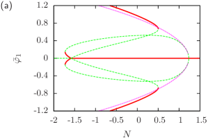
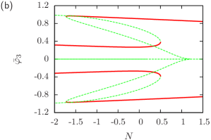
Figure 5: (Color online) The panels show the amplitudes (a) $\bar{\varphi}_{1}$ and (b) $\bar{\varphi}_{3}$ of the steady-state solutions of the two mode approximations to the concentration profile Eq. (18). Stable solutions are indicated by a solid red line, and the unstable ones by dashed green line. For comparison the dotted purple line in panel (a) also shows the single mode approximation Eq. (16).

IV.1.1 Single Mode

Taking into account only the modes $j=\pm 1$ leads to

$$\dot{\varphi}_{1}=-\left(N-\frac{\pi^{2}}{8}+\frac{\pi^{4}M^{2}}{16}\right)\varphi_{1}-\frac{3}{2}\varphi_{1}^{3}$$ (15)

It admits the stationary solutions $\varphi=0$ and the nontrivial solution

$$\bar{\varphi}=\frac{\pi}{2}\,\left(\frac{1}{3}-\frac{\pi^{2}M^{2}}{6}-\frac{8N}{3\pi^{2}}\right)^{1/2}$$ (16)

which ceases to exist at the critical point

$$N_{c}^{(1)}=\frac{\pi^{2}}{8}-\frac{\pi^{4}M^{2}}{16}$$ (17)

Already in this simplest conceivable framework it is not possible to have a stable diffusion profile when the parameter $N$ characterizing the strength of the temperature drift becomes too large. However, in this setting the amplitude $\bar{\varphi}$ of the supersaturation profile vanishes upon approaching $N_{c}$ rather than that the stable profile vanishes in a saddle node bifurcation as suggested by the findings summarized in Fig. 3.

IV.1.2 Two Modes

Taking into account the two leading order modes $j=\pm 1,\pm 3$ leads to

$$\dot{\varphi}_{1} = -\left(N-\;\;\frac{\pi^{2}}{8}+\;\;\;\frac{\pi^{4}M^{2}}{16}\right)\varphi_{1}-\frac{3}{2}\varphi_{1}^{3}+\frac{3}{2}\varphi_{1}^{2}\varphi_{3}-3\,\varphi_{1}\varphi_{3}^{2}$$ (18a)

$$\dot{\varphi}_{3} = -\left(N-\frac{9\pi^{2}}{8}+\frac{81\pi^{4}M^{2}}{16}\right)\varphi_{3}+\frac{9}{2}\varphi_{1}^{3}-27\,\varphi_{1}^{2}\varphi_{3}-\frac{27}{2}\varphi_{3}^{3}$$ (18b)

For the case of narrow interfaces $M=0$ its steady-state solutions are plotted in Fig. 5:
There still is a solution whose amplitude continuously disappears upon approaching the critical parameter value $N_{c}^{(1)}=\pi/8\simeq 1.2337$ found in Eq. (17). Close to the bifurcations its amplitudes are very close to the one of the single mode approximation (purple dotted line). However, this solution is now correctly identified as an unstable solution where the concentration lies within the spinodal region all the time. It corresponds to one of the closed orbits in the center region of Fig. 4.
Moreover, the two mode model admits two qualitatively new types of solutions. For all $N>0$ there is a stable solution $\bar{\varphi}_{1}=0$ and $\bar{\varphi}_{3}=\frac{\pi}{2}\,\left(\frac{1}{3}-\frac{\pi^{2}M^{2}}{6}-\frac{8}{3\pi^{2}}\;\frac{N}{9}\right)^{1/2}$ which amounts to the single mode approximation of a system of height $\Lambda/3$ rather than $\Lambda$.
In addition, for small $N$ there are two (symmetry-related) pairs of non-trivial solutions, which disappear in saddle-node bifurcations at $N_{c}^{(2)}\simeq 0.5031$, which is remarkably close to the exact value $N_{c}=(\sqrt{3}-1)^{2}\simeq 0.5359$ obtained in Eq. (12) (cf. Fig. 2). Beyond this value of $N$ diffusion is too slow to remove the supersaturation from a domain of size $\Lambda$, and the system approaches the stable fixed point with vanishing amplitude $\bar{\varphi}_{1}$.

The saddle node bifurcation at $N_{c}$ and the subsequent decay towards a solution with domains of size $\Lambda/3$ has a simple physical interpretation. It amounts to nucleation of new domains close to the top and bottom of the system where supersaturation is largest, such that the domain size is reduced to one third of its previous value and diffusive relaxation can again keep track with the driving of the system. When relaxing the constraint of translational invariance in horizontal direction, nucleation would of course give rise to a cloud of droplets rather than a full two-dimensional layer of material. A discussion of the related instabilities and feedback-mechanisms lie outside the scope of the present work. First steps to their understanding have been suggested in Vollmer et al. (2007), and a more detailed analysis will be given in forthcoming work. At this point we conclude that the two-mode model faithfully describes the breakdown of stable diffusion by a saddle-node bifurcation. Even though the values of the supersaturation are reproduced only in a crude approximation (dashed lines in Fig. 3) its prediction of the critical point is off by less than $7$%. Adding more modes in first place gives a more realistic description of the stable solutions remaining for $N>N_{c}$ and in the completely analogous saddle node bifurcations leading to breakdown of diffusion in these structures, when $N$ becomes still larger.

V Discussion

In this paper we have studied the diffusive transport in binary mixtures in response to ultra-slow cooling. Starting from the generic $\phi^{4}$ model of binary fluid mixtures we showed

• that stable diffusion is only possible up to a critical parameter value Eq. (12) where the stable diffusion profiles merges with an unstable profile, and disappears in a saddle-node bifurcation.

• This prediction of the critical value applies whenever the concentration dependence of diffusivity is well-approximated by an even 2nd order polynomial.

• In the limit of sharp interfaces the steady state profiles may be represented in the form of flow diagrams Figs. 4 and 7. Since the flow is topologically stable, the findings are not restricted to the specific model but are robust to changes in the phase boundaries and concentration dependence of the diffusivity.

• An expansion of the model in a Fourier series shows that the picture also applies when the forth order derivatives are included in the diffusion equation (5) that are needed to account for the finite width of the interface between coexisting phases.

• When approaching the critical parameter value of the saddle-node bifurcation the concentration profile becomes unstable with respect to nucleation of droplets, which will break the horizontal translation invariance assumed in the present study.

The two-mode approximation of the concentration profiles faithfully describes the approach to the bifurcation, and may hence serve as a starting point to further explore the nucleation of droplets and its feedback on the transport of supersaturation.

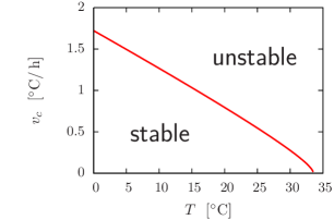
Figure 6: (Color online) The solid red line gives an estimate (19) where the saddle node bifurcation leads to a breakdown of continuous diffusive demixing in the mixtures of hexane and methanol considered in detail in Ref. Auernhammer et al. (2005). The label ‘stable’ marks the range of heating rates $v$ where diffusion keeps pace with the generation of supersaturation by the change of temperature. For larger heating rates (region marked as ‘unstable’) supersaturation will become so large that droplets are nucleated.

We conclude the present study by estimating the maximal cooling rates where a mixture can still catch up with the change of temperature in a system of lateral extension $\Lambda\simeq 1\;$cm. For a mixture of methanol and hexane the equilibrium diffusion coefficient at the considered temperatures is of the order of $D\simeq 10^{-5}$cm²/s. In view of Eqs. (4) and (6a) the system can only smoothly follow the change of temperature when the cooling rate the cooling rate does not exceed a critical value

$$v_{c}\equiv\left.\frac{{\mathrm{d}}T}{{\mathrm{d}}t}\right|_{c}\simeq\frac{N_{c}}{\partial_{T}\phi_{0}}\;\frac{D}{\Lambda^{2}}$$ (19)

By comparison with the phase diagram for the mixtures (cf. Fig. 5 in Auernhammer et al. (2005)) one finds that for all experimentally accessible temperatures the cooling rate must not exceed a few K/h (Fig. 6). For other binary mixtures these numbers will be of the same order, and for polymer solutions where the diffusion coefficient is still three orders of magnitude smaller the cooling rate must not exceed a few Kelvin per month.

in view of the results summarized in Fig. 6 this study strongly suggest that complex time-dependent nonlinear behavior must be considered as the typical response of a binary liquid which is driven into the coexistence region by a temperature ramp. Only when special precautions are taken, or when one approaches a region in the phase diagram where temperature changes do not induce changes of the composition diffusion can keep the system close to equilibrium.

Appendix A Asymmetric phase diagrams

In Auernhammer et al. (2005) it is shown that binary mixtures with a symmetric coexistence region are described by Eq. (8), even when the critical point does not correspond to equal volume fractions of both phases. An asymmetric miscibility gap can be characterized by the temperature dependence of the mean value $\bar{\phi}(T)$ of the coexisting compositions. It gives rise to an additional source term $\zeta\equiv\phi_{0}^{-1}\,\partial_{t}\bar{\phi}$ in the diffusion equation, which breaks the $\varphi\to-\varphi$ symmetry. Absorbing $\xi\Lambda^{2}/D$ again into the length scale and concentrating on the case $M\ll 1$ (i. e., $\delta\ll\Lambda$) one obtains

$$\partial_{z}\left[\frac{3\varphi^{2}-1}{2}\>\partial_{z}\varphi\right]\simeq\varphi-\frac{\zeta}{\xi}.$$ (20)

The flow diagram for the stationary concentration profiles for $\zeta/\xi=0.067$ is shown in Fig. 7. In comparison to the symmetric case Fig. 4 the heteroclinic connection between the saddle points on the spinodal disappear. This leads to a rearrangement of the flow in the unstable region $-\varphi_{s}<\varphi<\varphi_{s}$. On the other hand, there are only minor changes in the profiles outside this range, and the criterion $|\varphi^{\prime}(0)|\leq 1$ to obtain a stable diffusive profile remains valid to a very good accuracy.

Figure 7: (Color online) Flow diagram of Eq. (20) for $\zeta/\xi=0.067$. All other parameters are the same as in Fig. 4.

Appendix B Mode expansion for the diffusion equation

When inserting the ansatz (13) into the nonlinear diffusion equation (5) only the nonlinear terms take some effort to evaluate. We observe that

$$\partial_{z}\left[\frac{3\varphi^{2}-1}{2}\>\partial_{z}\varphi\right]=3\varphi\>(\partial_{z}\varphi)^{2}+\frac{3}{2}\varphi^{2}\>\partial_{z}^{2}\varphi-\frac{1}{2}\partial_{z}^{2}\varphi$$

and evaluate the terms one after the other.

Observing that $\partial_{z}\varphi=\sum_{j}^{\prime}j\,\varphi_{j}\,\cos\frac{\pi jz}{2}$ we thus obtain

$$3\varphi\>(\partial_{z}\varphi)^{2} = \frac{6}{\pi}\;{\sum_{jkl}}^{\prime}kl\;\varphi_{j}\,\varphi_{k}\,\varphi_{l}\;\sin\frac{\pi jz}{2}\;\cos\frac{\pi kz}{2}\;\cos\frac{\pi lz}{2}$$

$$= \frac{3}{2\pi}\;{\sum_{jkl}}^{\prime}kl\;\varphi_{j}\,\varphi_{k}\,\varphi_{l}\;\left[\sin\frac{\pi(j+k+l)z}{2}+\sin\frac{\pi(j-k-l)z}{2}+\sin\frac{\pi(j+k-l)z}{2}+\sin\frac{\pi(j-k+l)z}{2}\right]$$

Using the antisymmetry of $\varphi_{j}$ and shifting the summation index this yields

$$3\varphi\>(\partial_{z}\varphi)^{2} = \frac{6}{\pi}\;{\sum_{jkl}}^{\prime}kl\;\varphi_{j}\,\varphi_{k}\,\varphi_{l}\;\sin\frac{\pi(j+k+l)z}{2}$$ (21a)

$$= \frac{6}{\pi}\;{\sum_{jkl}}^{\prime}kl\;\varphi_{j-k-l}\,\varphi_{k}\,\varphi_{l}\;\sin\frac{\pi jz}{2}$$

By an analogous calculation one finds

$$\frac{3}{2}\varphi^{2}\>\partial_{z}^{2}\varphi=\frac{6}{\pi}\;{\sum_{jkl}}^{\prime}\frac{k^{2}}{2}\;\varphi_{j-k-l}\,\varphi_{k}\,\varphi_{l}\;\sin\frac{\pi jz}{2}$$ (21b)

Collecting the expansion coefficients of the Fourier series then immediately leads to Eq. (14).

References

- Lifshitz and Slyozov (1961) I. Lifshitz and V. Slyozov, J. Phys. Chem. Solids 19, 35 (1961).
- Siggia (1979) E. D. Siggia, Phys. Rev. A 20, 595 (1979).
- Gunton et al. (1983) J. Gunton, M. S. Miguel, and P. Sahni, in Phase Transitions and Critical Phenomena, edited by C. Domb and J. Lebowitz (Academic Press, New York, 1983), vol. 8, p. 267.
- Bray (1994) A. Bray, Adv. Phys. 43, 357 (1994).
- Binder (1998) K. Binder, J. of Non-Equil. Thermody. 23, 1 (1998).
- Onuki (2002) A. Onuki, Phase Transition Dynamics (Cambridge, Cambridge, 2002).
- Tanaka (1994) H. Tanaka, Phys. Rev. Lett. 72, 3690 (1994), polymer.
- Tanaka and Sighuzi (1995) H. Tanaka and T. Sighuzi, Phys. Rev. Lett. 75, 874 (1995), periodically driven above and below stability point.
- Vollmer et al. (1997a) D. Vollmer, J. Vollmer, and R. Strey, Europhys. Lett. 39, 245 (1997a).
- Vollmer et al. (1997b) D. Vollmer, R. Strey, and J. Vollmer, J. Chem. Phys. 107, 3619 (1997b).
- Vollmer et al. (1997c) J. Vollmer, D. Vollmer, and R. Strey, J. Chem. Phys. 107, 3627 (1997c).
- Vollmer and Vollmer (1999) J. Vollmer and D. Vollmer, Faraday Disc. 112, 51 (1999).
- Wagner and Yeomans (1998) A. Wagner and J. M. Yeomans, Phys. Rev. Lett. 80, 1429 (1998).
- Kendon et al. (1999) V. Kendon, J.-C. Desplat, P. Bladon, and M. Cates, Phys. Rev. Lett. 83, 576 (1999), no indication that Re is self-limiting.
- Puri and Binder (2001) S. Puri and K. Binder, Phys. Rev. Lett. 86, 1797 (2001), numerical studies, effects of wetting.
- Chaikin and Lubensky (2000) P. M. Chaikin and T. C. Lubensky, Principles of Condensed Matter Physics (Cambridge, Cambridge, 2000).
- Wong and Knobler (1981) N.-C. Wong and C. M. Knobler, Phys. Rev. A 24, 3205 (1981), growth of droplets, Siggia-growth, Lifshitz-Slyoyov growth.
- Chou and Goldburg (1981) Y. Chou and W. Goldburg, Phys. Rev. A 23, 858 (1981), isobutyric-acid/water, 2,6lutidine/water, light scattering, structure factor.
- Joshua and Goldburg (1985) M. Joshua and W. Goldburg, Phys. Rev. A 31, 3857 (1985), periodically driven through consolute point, mean-field behavior.
- Cumming et al. (1990) A. Cumming, P. Wiltzius, and F. S. Bates, Phys. Rev. Lett. 65, 863 (1990).
- Cates et al. (2003) M. Cates, J. Vollmer, A. Wagner, and D. Vollmer, Phil. Trans. Roy. Soc. (Lond.) Ser. A 361, 793 (2003), convection, Bernard-analogon.
- Auernhammer et al. (2005) G. K. Auernhammer, D. Vollmer, and J. Vollmer, J. Chem. Phys. 123, 134511 (2005).
- Vollmer et al. (2007) J. Vollmer, G. K. Auernhammer, and D. Vollmer, Phys. Rev. Lett. 98, 115701 (2007), URL http://link.aps.org/abstract/PRL/v98/e115701.
- Sparks et al. (1993) R. S. Sparks, H. E. Huppert, T. Kozaguchi, and M. A. Hallwood, Nature 361, 246 (1993), magma chamber.
- Heimburg et al. (2000) T. Heimburg, S. Z. Mirzaev, and U. Kaatze, Phys. Rev. E 62, 4963 (2000).
- Vollmer et al. (2002) D. Vollmer, J. Vollmer, and W. Wagner, Phys. Chem. Chem. Phys. 4, 1380 (2002).
- Turchanin and Freyland (2004) A. Turchanin and W. Freyland, Chem. Phys. Lett. 387, 106 (2004).
- Turchanin et al. (2004) A. Turchanin, R. Tsekov, and W. Freyland, J. Chem. Phys. 120, 11171 (2004).
- Wagner et al. (2003) A. Wagner, M. E. Cates, and J. Vollmer (2003).
- Arnold (2008) V. I. Arnold, Ordinary Differential Equations (Springer, Berlin, 2008), 2nd ed.