On Gautschi’s conjecture for generalized Gauss-Radau and Gauss-Lobatto formulae

Abstract

Recently, Gautschi introduced so-called generalized Gauss-Radau and Gauss-Lobatto formulae which are quadrature formulae of Gaussian type involving not only the values but also the derivatives of the function at the endpoints. In the present note we show the positivity of the corresponding weights; this positivity has been conjectured already by Gautschi.

As a consequence, we establish several convergence theorems for these quadrature formulae.

Keywords. Quadrature formula, Gauss-Radau formula, Gauss-Lobatto formula, orthogonality with varying weights.

AMS subject classifications. 65D30, 42C05.

1 Introduction

In a recent paper [4], Gautschi considered so-called generalized Gauss-Radau and Gauss-Lobatto formulae which are quadrature formulae of Gaussian type, i.e., having a highest possible degree of exactness, and involving not only the values but also the derivatives of the function at the endpoints of the interval of integration. Such formulae are of the form

$$\int f(t)\,d\lambda(t) = \sum_{j=0}^{r-1}\lambda_{0}^{(j)}f^{(j)}(a)+\sum_{j=1}^{n}\lambda_{j}f(\tau_{j})+\sum_{j=0}^{s-1}(-1)^{j}\lambda_{n+1}^{(j)}f^{(j)}(b)+R_{n,r,s}(f)$$ (1)

$$=: Q_{n,r,s}(f)+R_{n,r,s}(f),$$

where $\lambda$ is a positive measure with support being a subset of $[a,b]$ having an infinite number of points of increase in $(a,b)$, and the integers $r,s\geq 0$ are the multiplicities of the endpoints $a$ and $b$, respectively. In what follows we will also allow the case $a=-\infty$ (or $b=+\infty$) of a possibly unbounded support in which case only $r=0$ (or $s=0$, respectively) is considered, that is, the corresponding sum in $Q_{n,r,s}(f)$ does vanish.

It is well-known and easily verified that our requirement of highest possible degree of exactness leads to a unique quadrature formula of the form (1) with degree of exactness being equal to $2n+r+s-1$

$$\forall f\in\mathbb{P}_{2n+r+s-1}:\qquad R_{n,r,s}(f)=0,$$ (2)

where here and in what follows $\mathbb{P}_{m}$ denotes the space of real polynomials of degree at most $m$. Here the free nodes $\tau_{j}$ have to be chosen as to be the simple zeros of the $n$th orthogonal polynomial with respect to the modified measure $(x-a)^{r}(b-x)^{s}d\alpha(x)$ on $(a,b)$ being clearly positive, and hence $\tau_{j}\in(a,b)$. Indeed, we get for $Q_{n,0,0}$ the classical Gaussian quadrature rule, for $Q_{n,1,0}$ and $Q_{n,0,1}$ the Gauss-Radau formulae and for $Q_{n,1,1}$ the Gauss-Lobatto formula. For all these classical quadrature formulae it is known that the weights $\lambda_{1},...,\lambda_{n}$ and possibly $\lambda_{0}^{(0)},\lambda_{n+1}^{(0)}$ are strictly positive. The generalized Gauss-Radau (Gauss-Lobatto) formulae of [4] are obtained for $s=0$ (and $r=s$, respectively).

Based on extensive numerical experiments for Jacobi, Laguerre and elliptic Chebyshev measures using the numerical tools and methods described in [3], Gautschi conjectured in [4, Section 2.2 and Section 3.2] that the weights of the generalized Gauss-Radau and Gauss-Lobatto formulae are all strictly positive. He proved himself this conjecture for the inner weights $\lambda_{1},...,\lambda_{n}$ as well as for some boundary weights, namely $\lambda_{0}^{(r-1)},\lambda_{0}^{(r-2)}>0$ for the generalized Gauss-Radau formulae $Q_{n,r,0}$, and $\lambda_{0}^{(r-1)},\lambda_{0}^{(r-2)},\lambda_{n+1}^{(r-1)},\lambda_{n+1}^{(r-2)}>0$ for the generalized Gauss-Lobatto formulae $Q_{n,r,r}$. However, the sign of the other weights remained an open question.

The aim of this paper is to show in Theorem 1 below that Gautschi’s conjecture is true, namely, all weights in the quadrature formulae $Q_{n,r,s}$ are strictly positive. For this we will show the slightly stronger result that suitable underlying Lagrange polynomials (in the Hermite sense) do not change sign in $(a,b)$. As a consequence, we obtain in Corollary 4 convergence of the quadrature $Q_{n,r,s}(f)$ for fixed $r,s$ and $n\to\infty$ for sufficiently differentiable functions $f$. The case of $r,s,n\to\infty$ is discussed in Theorem 7 where we establish a geometric rate of convergence for analytic $f$.

Before stating and proving our results in the next sections, we should mention that generalized Gauss-Radau and Gauss-Lobatto formulae are of major interest in different applications, and in particular in moment preserving spline approximation on a compact interval $[a,b]=[0,1]$, see [2], [3, § 3.3], and [4, § 4]: given a function $f\in\mathcal{C}^{m+1}([0,1])$ with moments $\mu_{j}=\int_{0}^{1}t^{j}f(t)\,dt$, we are looking for a partition $0=\tau_{0}<\tau_{1}<...<\tau_{n}<\tau_{n+1}=1$ and a spline $\sigma$ of class $\mathcal{C}^{m-1}$ being piecewise $\mathbb{P}_{m}$ on each $[\tau_{j},\tau_{j+1}]$ for $j=0,1,...,n$ and having the same moments

$$\forall j=0,1,...,N:\qquad\int_{0}^{1}t^{j}\sigma(t)\,dt=\mu_{j},$$ (3)

with $N$ as large as possible, or in other words, the error $f-\sigma$ is orthogonal to $\mathbb{P}_{N}$ with respect to Lebesgue measure. By [3, Theorem 3.61], such a spline $\sigma$ exists for $N=2n+m$ if and only if the measure $d\lambda(t)=(-1)^{m+1}f^{(m+1)}(t)/(m!)\,dt$ on $[0,1]$ has a generalized Gauss-Radau quadrature formula $Q_{n,m+1,m+1}$ as in (1), and in this case the spline is given by the quadrature data via

$$\sigma(t)=\sum_{j=1}^{n}\lambda_{j}(\tau_{j}-t)_{+}^{m}\,+\,\sum_{j=0}^{m}\frac{(t-1)^{j}}{j!}[f^{(j)}(1)+(-1)^{m}\,m!\,\lambda_{n+1}^{(m-j)}].$$

2 Positivity of the weights

Theorem 1

All weights in the Gauss-type quadrature formula $Q_{n,r,s}$ given in (1) are strictly positive for all integers $n,r,s\geq 0$

$$j=1,2,...,n: \lambda_{j}>0,$$ (4)

$$j=0,1,2,...,r-1: \lambda_{0}^{(j)}>0,$$ (5)

$$j=0,1,2,...,s-1: \lambda_{n+1}^{(j)}>0.$$ (6)

• The property (4) has already been established by Gautschi [4], for the sake of completeness we repeat here the proof: consider

  $$p_{j}(t)=\frac{\omega_{j}(t)}{\omega_{j}(\tau_{j})},\quad\omega_{j}(t)=(t-a)^{r}(b-t)^{s}\prod_{k=1,k\neq j}^{n}(\tau_{k}-t)^{2},$$

  then it is clear by construction that $p_{j}(\tau_{j})=1$, and $p_{j}\in\mathbb{P}_{2n+r+s-2}$ is non negative on $(a,b)$. According to (2), we may conclude that $R_{n,r,s}(p_{j})=0$, and thus

  $$\lambda_{j}=Q_{n,r,s}(p_{j})=\int p_{j}(t)d\lambda(t)>0,$$

  as claimed in (4).

  For a proof of (5), consider the polynomial

  $$P_{j}(t)=P_{n,r,s,a,j}(t)=\frac{(t-a)^{j}}{j!}\Omega_{r-j-1}(t)\omega(t),\quad\omega(t)=(b-t)^{s}\prod_{k=1}^{n}(\tau_{k}-t)^{2},$$ (7)

  where $\Omega_{m}$ denotes the $m$th partial sum of the Taylor expansion of $1/\omega$ at $t=a$. Writing shorter

  $$D^{k}_{c}f=\frac{f^{(k)}(c)}{k!},$$

  we observe that, by construction,

  $$\forall k=1,...,n:\,\,D^{0}_{\tau_{k}}P_{j}=0,\quad\forall k=0,...,s-1:\,\,D^{k}_{b}P_{j}=0,\quad\forall k=0,...,j-1:\,\,D^{k}_{a}P_{j}=0.$$

  Furthermore, for $k=j,j+1,...,r-1$ we find by the Leibniz product rule and by definition of $\Omega_{m}$ that

  $$D^{k}_{a}P_{j}=\sum_{\ell=0}^{k}\Bigl{[}D^{\ell}_{a}\frac{(t-a)^{j}}{j!}\Bigr{]}\,\Bigl{[}D^{k-\ell}_{a}(\Omega_{r-j-1}\omega)\Bigr{]}=\frac{1}{j!}D^{k-j}_{a}(\Omega_{r-j-1}\omega)=\frac{1}{j!}\delta_{k-j,0}.$$

  Since in addition $P_{j}\in\mathbb{P}_{2n+r+s-1}$, we may conclude that

  $$\lambda_{0}^{(j)}=\lambda_{0}^{(j)}\,j!\,D_{a}^{j}P_{j}=Q_{n,r,s}(P_{j})=\int P_{j}(t)\,d\lambda(t).$$ (8)

  In order to discuss the sign of the expression on the right, we need the following auxiliary result.

  Lemma 2

  Let $P(t)=\prod_{j=1}^{m}(x_{j}-t)$, with $x_{1},...,x_{m}\in(c,+\infty)$, then

  $$\forall\ell=0,1,...:\qquad D_{c}^{\ell}\Bigl{(}\frac{1}{P}\Bigr{)}>0.$$

  • For $m=1$ we find that $D_{c}^{\ell}\bigl{(}\frac{1}{P}\bigr{)}=\frac{1}{(x_{1}-c)^{\ell+1}}>0$. The general case follows by induction on $m$ using the Leibniz product rule. $\Box$

  As a consequence of the preceding lemma, we find that

  $$\Omega_{m}(t)=\sum_{\ell=0}^{m}(t-a)^{\ell}D_{a}^{\ell}\Bigl{(}\frac{1}{\omega}\Bigr{)}$$

  is strictly positive on $(a,b)$ for all $m\geq 0$, and thus $P_{j}$ defined in (7) is also non negative in $(a,b)$. It follows from (8) that $\lambda_{0}^{(j)}>0$, as claimed in (5).

  Finally, for a proof of (6) we observe that the variable transformation $t^{\prime}=-t$ allows to exchange the roles of $(r,a,\lambda_{0}^{(j)})$ and $(s,b,\lambda_{n+1}^{(j)})$ in the quadrature formula (1), and in particular gives a factor $(-1)^{j}$ for the $j$th derivative. Hence the assertion (6) follows from (5), but it is also straight forward to give a direct proof following the above lines. $\Box$

Remark 3

Notice that also $D_{\tau_{k}}^{1}P_{j}=0$ for $k=1,2,...,n$. Thus, for polynomial interpolation (in the sense of Hermite) at the node $a$ with multiplicity $r$, the nodes $\tau_{1},...,\tau_{n}$ with multiplicity $2$, and $b$ with multiplicity $s$, we have shown implicitly that the Lagrange polynomials $P_{j}=P_{n,r,s,a,j}$ associated with the $j$th derivative at $a$ do not change sign on $[a,b]$. It follows by symmetry that the Lagrange polynomial $P_{n,r,s,b,j}$ associated with the $j$th derivative at $b$ has constant sign $(-1)^{j}$ on $[a,b]$. However, the Lagrange polynomials associated with $\tau_{j}$ may very well change sign on $(a,b)$.

The positivity of the quadrature weights is the essential key for proving the following convergence result both for generalized Gauss-Radau and for Gauss-Lobatto formulae.

Corollary 4

Let $[a,b]$ be compact, and $q:=\max\{r-1,s-1\}$. Then for any $f\in\mathcal{C}^{q}([a,b])$ we have

$$\lim_{n\to\infty}Q_{n,r,s}(f)=\int f(t)\,d\lambda(t).$$

• In the sequal of this proof we suppose that $r,s\geq 1$, the extension of the proof for $r=0$ or $s=0$ is straight forward. It is not difficult to see that the space $X=\mathcal{C}^{q}([a,b])$ equipped with the norm

  $$\|f\|=\max_{0\leq j\leq q}\max_{x\in[a,b]}|f(x)|$$

  gives a Banach space: the completeness follows immediately from the well-known completeness of the space $\mathcal{C}([a,b])$ with respect to the maximum norm on $[a,b]$, see, e.g., [7, p. 258]. Also, from [1, Theorem 6.3.2] it follows that polynomials are dense in $(X,\|\cdot\|)$. Hence we are prepared to apply the Banach-Steinhaus Theorem: for $f$ being a polynomial of degree $k$, we obtain from (2) that

  $$\forall n>\frac{k-r-s}{2}:\qquad Q_{n,r,s}(f)=\int f(t)\,d\lambda(t),$$

  i.e., we have convergence for a dense subset of $(X,\|\cdot\|)$. For obtaining convergence in $X$ it only remains to show that the norm of the linear functionals $Q_{n,r,s}$ is bounded uniformly in $n$. Writing more explicitly $\lambda_{0}^{(j)}(n),\lambda_{j}(n),\lambda_{n+1}^{(j)}(n)$ for the quadrature weights occurring in (1), we obtain the simple upper bound

  $$\|Q_{n,r,s}\|\leq\sum_{j=0}^{r-1}\lambda_{0}^{(j)}(n)+\sum_{j=1}^{n}\lambda_{j}(n)+\sum_{j=0}^{s-1}\lambda_{n+1}^{(j)}(n),$$ (9)

  since, according to Theorem 1, all weights occurring in these sums are positive. We observe that

  $$\lambda_{0}^{(0)}(n)+\sum_{j=1}^{n}\lambda_{j}(n)+\lambda_{n+1}^{(0)}(n)=Q_{n,r,s}(1)=\int d\lambda(t)<\infty.$$

  For the remaining terms we consider the polynomial (not depending on $n$)

  $$P(x):=\sum_{j=1}^{r-1}P_{0,r,s,a,j}(x)+\sum_{j=1}^{s-1}(-1)^{j}P_{0,r,s,b,j}(x)$$

  of degree $\leq r+s-1$, where we recall from Remark 3 that each term in the above sums, representing up to a sign a Lagrange polynomial in the sense of Hermite at the abscissa $a$ with multiplicity $r$ and $b$ with multiplicity $s$, is non negative on $[a,b]$. Hence this polynomial $P$ is also non negative on $[a,b]$, implying that, again by the positivity of the weights,

  $$\sum_{j=1}^{r-1}\lambda_{0}^{(j)}(n)+\sum_{j=1}^{s-1}\lambda_{n+1}^{(j)}(n)\leq Q_{n,r,s}(P)=\int P(t)\,d\lambda(t)$$

  for all $n\geq 0$, where in the last equality we have used (2). Hence the expression on the right of (9) is bounded uniformly in $n$, and the Banach-Steinhaus Theorem allows us to conclude that there is convergence as claimed in the assertion of Corollary 4. $\Box$

Remark 5

By using classical arguments we may also estimate the rate of convergence of our quadrature formula: according to (2), we find the following bound for the error

$$|R_{n,r,s}(f)|\leq\Bigl{(}\int d\lambda(t)+\|Q_{n,r,s}\|\Bigr{)}\,\inf_{p\in\mathbb{P}_{2n+r+s-1}}\|f-p\|.$$ (10)

Here we can give a quite rough explicit upper bound for $\|Q_{n,r,s}\|$ which is independent of $n$: by having a closer look at the construction of the polynomials $P_{0,r,s,a,j}$ from (7) we see that

$$\forall x\in[a,b]:\qquad 0\leq P_{0,r,s,a,j}(x)\leq\frac{(x-a)^{j}}{j!}\sum_{\ell=0}^{r-j-1}\frac{(x-a)^{\ell}}{(b-a)^{s+\ell}}\leq r(b-a)^{r},$$

and a similar bound for $(-1)^{j}P_{0,r,s,b,j}(x)$. Consequently, we learn from the previous proof and especially from (9) that

$$\|Q_{n,r,s}\|\leq\Bigl{(}1+r^{2}(b-a)^{r}+s^{2}(b-a)^{s}\Bigr{)}\int d\lambda(t).$$ (11)

Using (10) and (11), it is possible to show also convergence for a composite quadrature rule based on suitably shifted and scaled counterparts of $Q_{n,r,s}$, and to derive an explicit rate of convergence in terms of the size of the largest underlying subinterval.

3 Rate of convergence for analytic functions

Denote by $P_{f}\in\mathbb{P}_{2n+r+s-1}$ the polynomial interpolating $f$ with multiplicity $r$ in $a$, multiplicity $s$ in $b$ and multiplicity $2$ at the other abscissae $\tau_{j}$ occurring in (1) for $j=1,...,n$, then using the Cauchy error formula for polynomial interpolation we get from (2) that the error for our quadrature formula for $f\in\mathcal{C}^{2n+r+s}([a,b])$ may be written in terms of divided differences as

$$R_{n,r,s}(f) = \int\Bigl{(}f(t)-P_{f}(t)\Bigr{)}\,d\lambda(t)$$

$$= \int(t-a)^{r}(t-b)^{s}\prod_{j=1}^{n}(t-\tau_{j})^{2}[\underbrace{a,...a}_{r},\underbrace{\tau_{1},\tau_{1}}_{2},...,\underbrace{\tau_{n},\tau_{n}}_{2},\underbrace{b,...,b}_{s},t]f\,d\lambda(t)$$

$$= [a,...a,\tau_{1},\tau_{1},...,\tau_{n},\tau_{n},b,...,b,\xi_{n,r,s}]f\int(t-a)^{r}(t-b)^{s}\prod_{j=1}^{n}(t-\tau_{j})^{2}\,d\lambda(t)$$

$$= \frac{f^{(2n+r+s)}(\xi^{\prime}_{n,r,s})}{(2n+r+s)!}\int(t-a)^{r}(t-b)^{s}\prod_{j=1}^{n}(t-\tau_{j})^{2}\,d\lambda(t)$$

with $\xi_{n,r,s},\xi^{\prime}_{n,r,s}\in[a,b]$, since the polynomial factor in the integral is of unique sign. Denote by $p_{n,r,s}$ the orthonormal polynomial with respect to the modified weight $(t-a)^{r}(b-t)^{s}\,d\lambda(t)$. We suppose that $\lambda$ has the compact support $[-1,1]$ with $a\leq-1<1\leq b$, then it is well-known from, e.g., [6, Section 11.11] that

$$\limsup_{n\to\infty}|R_{n,0,0}(f)|^{1/n}\leq 1/\rho^{2}<1$$ (13)

provided that $f$ is analytic in the closed ellipse $\mathcal{E}_{\rho}$ with foci $\pm 1$ and half axes $(\rho\pm 1/\rho)/2$, and that this result is optimal for measures satisfying the Szegö condition. A similar rate is shown to be true for fixed $r,s>0$, and we are curious about the rate of convergence if $r=r_{n}$ and $s=s_{n}$ such that $r_{n}/n\to\alpha\geq 0$, $s_{n}/n\to\beta\geq 0$.

We first notice that $\xi_{n,r,s}\in[-1,1]$ in (3). Hence, for a (set of) contour(s) $\mathcal{C}$ encercling once $[-1,1]$ and $a,b$ and staying in a neighborhood of $[a,b]$ where $f$ is analytic, we get from the Cauchy formula for divided differences and from (3)

$$R_{n,r_{n},s_{n}}(f)=\frac{1}{2\pi i}\int_{\mathcal{C}}\frac{f(z)}{(z-\xi_{n,r_{n},s_{n}})(z-a)^{r_{n}}(b-z)^{s_{n}}p_{n,r_{n},s_{n}}(z)^{2}}dz,$$

and thus

$$\limsup_{n\to\infty}|R_{n,r_{n},s_{n}}(f)|^{1/n}\leq\limsup_{n\to\infty}\max_{z\in\mathcal{C}}\frac{1}{|z-a|^{\alpha}|z-b|^{\beta}|p_{n,r_{n},s_{n}}(z)|^{2/n}}.$$ (14)

Thus we are left with the question of $n$th roots asymptotics for orthogonal polynomials with varying weights, which has been the subject of a number of publications over the last twenty years, see, e.g., the monograph [8, Chapters III.6 and VII] of Saff and Totik or the monograph [9, Chapter 3] of Stahl and Totik. Since the negative logarithm of the absolute value of a polynomial is a logarithmic potential of some discrete measure, here the right tool to describe the $n$th root asymptotic is to consider a weighted equilibrium problem in logarithmic potential theory: the potential and the energy of a Borel measure $\mu$ with compact support are defined by

$$U^{\mu}(y)=\int\log(\frac{1}{|x-y|})\,d\mu(x),\qquad I(\mu)=\int\int\log(\frac{1}{|x-y|})\,d\mu(x)\,d\mu(y).$$

Define the external field $Q(x)=U^{\sigma}(x)$, $\sigma=\frac{\alpha}{2}\delta_{a}+\frac{\beta}{2}\delta_{b}$, with $\delta_{c}$ the Dirac unit point measure at $x=c$, then there exists a unique probability measure $\mu$ supported on $\Sigma=[-1,1]$ which under all such measures has minimal weighted energy $I(\mu)+2\int Q\,d\mu$, see [8, Theorem I.1.3]. By the same Theorem (see also [8, Theorem I.5.1]) we also have the equilibrium conditions that $U^{\mu}(x)+Q(x)$ is equal to some constant $F$ on the support of $\mu$, and $\geq F$ in $[-1,1]$. Then according to [5] (see also [9])

$$\Bigl{(}\limsup_{n\to\infty}\max_{z\in\mathcal{C}}\frac{1}{|z-a|^{\alpha}|z-b|^{\beta}|p_{n,r_{n},s_{n}}(z)|^{2/n}}\Bigr{)}\leq\exp\Bigl{(}2\,\sup_{z\in\mathcal{C}}\Bigl{(}U^{\mu}(z)+Q(z)-F\Bigr{)}\Bigr{)},$$ (15)

with equality iff the starting measure of orthogonality $\lambda$ is sufficiently regular.

For our external field, the extremal measure may be found explicitly: since $Q$ is convex on $[-1,1]$, it follows from [8, Theorem IV.1.11] that the support of $\mu$ is an interval of the form $[A,B]$, with $-1\leq A<B\leq 1$, and also $a<A$ and $B<b$ since $Q$ becomes $+\infty$ at $a$, $b$ and thus in a neighborhood of these points we may not have equality in the equilibrium condition.

Lemma 6

Denoting by $z\mapsto\phi(z)=(2z-A-B+2\sqrt{(z-A)(z-B)})/(B-A)$ the conformal Riemann map sending the exterior of $[A,B]$ onto the exterior of the closed unit disk, then we have for $z\in\mathbb{C}$

$$\exp(2(U^{\mu}(z)+Q(z)-F))=\frac{1}{|\phi(z)|^{2}}\Bigl{|}\frac{1-\phi(z)\phi(a)}{\phi(z)(\phi(z)-\phi(a))}\Bigr{|}^{\alpha}\Bigl{|}\frac{1-\phi(z)\phi(b)}{\phi(z)(\phi(z)-\phi(b))}\Bigr{|}^{\beta},$$ (16)

where $-1\leq A<B\leq 1$ are defined by the system

$$\frac{\alpha}{2}(\sqrt{\frac{A-a}{B-a}}-1)+\frac{\beta}{2}(\sqrt{\frac{b-A}{b-B}}-1)\left\{\begin{array}[]{ll}=1&\mbox{if $B<1$,}\\ \leq 1&\mbox{if $B=1$,}\end{array}\right.$$

$$\frac{\alpha}{2}(\sqrt{\frac{B-a}{A-a}}-1)+\frac{\beta}{2}(\sqrt{\frac{b-B}{b-A}}-1)\left\{\begin{array}[]{ll}=1&\mbox{if $A>-1$,}\\ \leq 1&\mbox{if $A=-1$.}\end{array}\right.$$

• Denote by $\widehat{\sigma}$ the balayage measure of $\sigma$ onto $[A,B]$, then by [8, Theorem II.4.4], $\mu+\widehat{\sigma}$ is a positive measure of total mass $(1+\frac{\alpha}{2}+\frac{\beta}{2})$ supported on $[A,B]$, and from the equilibrium conditions we know that its potential is constant quasi everywhere on $[A,B]$. However, by, e.g., [8, Theorem I.1.3], the only measure satisfying this relation is $(1+\frac{\alpha}{2}+\frac{\beta}{2})\omega_{[A,B]}$, with $\omega_{[A,B]}$ the Robin measure of $[A,B]$, i.e., the equilibrium measure with external field $0$ on $[A,B]$. Hence from [8, Eqns. (II.4.32) and (II.4.35)] and the fact that $U^{\mu}+Q-F$ equals zero on $[A,B]$ we may conclude that

  $$U^{\mu}(z)+Q(z)-F=\frac{\alpha}{2}g_{[A,B]}(z,a)+\frac{\beta}{2}g_{[A,B]}(z,b)-(1+\frac{\alpha}{2}+\frac{\beta}{2})g_{[A,B]}(z,\infty),$$

  where by $x\mapsto g_{[A,B]}(x,y)$ we denote the Green function of the domain $\mathbb{C}\setminus[A,B]$ with pole at $y\not\in[A,B]$. Taking into account the link [8, Eqn. (II.4.45)] between the Green function and the Riemann map, relation (16) follows. Finally, the so-called F-functional of [8, Theorem IV.1.5]

  $$F(A,B) = \log(\frac{B-A}{4})-\frac{1}{\pi}\int_{A}^{B}\frac{Q(x)\,dx}{\sqrt{(x-A)(B-x)}}$$

  $$= (1+\frac{\alpha}{2}+\frac{\beta}{2})\log(\frac{B-A}{4})+\frac{\alpha}{2}g_{[A,B]}(a,\infty)+\frac{\beta}{2}g_{[A,B]}(b,\infty)$$

  must take its global maximum on $-1\leq A<B\leq 1$ at the endpoints of the support of the extremal measure $\mu$. Taking partial derivatives, we arrive at the given system of equations and inequalities for $A$, $B$ as in [8, Theorem II.4.4 and Lemma II.1.15], compare with [8, Example II.1.17] for the special case $a=-1$ and $b=1$ of Jacobi weights. $\Box$

   

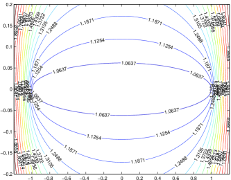
Figure 1: Level curves for different choices of the parameters $a,\alpha,b,\beta$: on the left we find the classical case $\alpha=\beta=0$, here $[A,B]=[-1,1]$ and the level lines are ellipses. On the right $\alpha=\beta=1$ and $b=-a=1$, the endpoints of the support of orthogonality, here the level sets for $\rho>1$ are connected with connected complement, in this case $B=-A\approx 0.86603$.

   

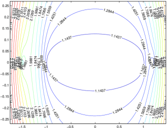
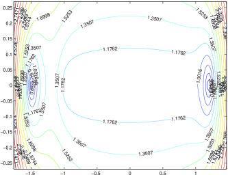
Figure 2: Level curves for different choices of the parameters $\alpha=\beta$: in both cases, $a=-1.5,b=1$, but on the left we find $\alpha=\beta=0.2$, on the right $\alpha=\beta=1$, leading to $[A,B]=[-1,1]$ in both cases. In particular, for small $\rho>1$ we find three connected components for our level sets.

   

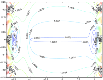
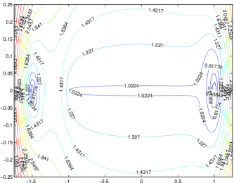
Figure 3: Level curves for different choices of the parameters $\beta$: in both cases, $a=-1.5,b=1$, $\alpha=1$, but $\beta=1$ on the left (leading to $[A,B]=[-1,0.8402]$), and $\beta=1.2$ on the right (leading to $[A,B]=[-1,0.79334]$). Here for small $\rho>1$ we find two connected components for our level sets.

In order to exploit Lemma 6, we have to consider for $\rho>1$ the (closed) level sets $\mathcal{E}_{\rho}(a,\alpha,b,\beta)$ being the complement of the set of $z\in\mathbb{C}\setminus[A,B]$ where the right-hand side of (16) is $<\rho^{-2}<1$. Notice that for $\alpha=\beta=0$ we have $[A,B]=[-1,1]$, and we obtain for the complement the reqirement $|\phi(z)|>\rho$, that is, $\mathcal{E}_{\rho}(a,0,b,0)$ coincides with the ellipses $\mathcal{E}_{\rho}$ considered before. Also, by the equilibrium conditions, $[-1,1]\cup\{a,b\}\subset\mathcal{E}_{\rho}(a,\alpha,b,\beta)$ for all $\rho>1$, and from the maximum principle for analytic functions we may conclude that $\mathcal{E}_{\rho}(a,\alpha,b,\beta)$ has a connected complement containing a neighborhood of infinity, and at most three connected components, one of them containing $a$ (if $\alpha>0$), a second $b$ (if $\beta>0$), and the third the interval $[-1,1]$, see Figure 2. Moreover, if $A>-1$ (and similarly $B<1$), then $\mu$ is also an extremal measure if we replace $\Sigma=[-1,1]$ by the larger set $[a,1]$, and hence $[a,1]\subset\mathcal{E}_{\rho}(a,\alpha,b,\beta)$, showing that there are only at most two connected components (see Figure 3).

If we choose as $\mathcal{C}$ the boundary of some level set $\mathcal{E}_{\rho}(a,\alpha,b,\beta)$ for some $\rho>1$, this (set of) contour(s) encircles once $a,b$, and the interval $[-1,1]$. A combination of (14), (15), and (16) leads to the following result.

Theorem 7

Suppose that $r_{n}/n\to\alpha\geq 0$, $s_{n}/n\to\beta\geq 0$, and let $f$ be analytic in $\mathcal{E}_{\rho}(a,\alpha,b,\beta)$ for some $\rho>1$, then

$$\limsup_{n\to\infty}|R_{n,r_{n},s_{n}}(f)|^{1/n}\leq\rho^{-2}.$$

One may show that again this estimate is best possible if the orthogonality measure $\lambda$ is sufficiently regular. In addition, if $\lambda$ satisfies the Szegő condition, then following [10] we may obtain strong asymptotics for the orthonormal polynomials $p_{n,r_{n},s_{n}}$, and hence with help of steepest descend an asymptotic equivalent of $|R_{n,r_{n},s_{n}}(f)|$.

Different examples for the level sets of the preceding theorem are given in Figure 1, Figure 2, and Figure 3. Though the shapes of these sets are quite different depending on the parameters, there seem to be clearly an indication: if the function $f$ is regular in larger neighborhoods around $a$ and $b$, but not in such a large neighborhood around for instance $0$ (which is true for instance for the function $f(z)=1/(1+z^{2})$), then by the choice of larger $\alpha,\beta$ one improves the rate of geometric convergence of our generalized Gauss-Lobatto quadrature formula.

References

- [1] P. J. Davis, Interpolation and Approximation, Blaisdell Publishing Co., New York, 1963.
- [2] M. Frontini, W. Gautschi, G.V. Milovanovic, Moment-preserving spline approximation of finite intervals, Numer. Math. 50 (1987), 503-518.
- [3] W. Gautschi, Orthogonal polynomials: computation and approximation, Numerical Mathematics and Scientific Computation, Oxford University Press, Oxford, 2004.
- [4] W. Gautschi, Generalized Gauss-Radau and Gauss-Lobatto formulae, BIT, 44 (2004) 711-720.
- [5] A.A. Gonchar and E.A. Rakhmanov, Equilibrium measure and the distribution of zeros of extremal polynomials, Math. Sb 125 (1984) 117-127.
- [6] P. Henrici, Applied and Computational Complex Analysis, vol. 2, Wiley, New York, 1977.
- [7] H. Queffélec, CI. Zuily, Eléments d’Analyse pour l’Agrégation, Masson, Paris, 1995.
- [8] E. B. Saff and V. Totik, Logarithmic Potentials with External Fields, Springer, Berlin, 1997.
- [9] H. Stahl and V. Totik, General Orthogonal Polynomials, Cambridge University Press, Cambridge, 1992.
- [10] V. Totik, Weighted approximation with varying weight. Lecture Notes in Mathematics 1569, Springer-Verlag, Berlin, 1994.