Neutrino Masses from Cosmological Probes
in Interacting Neutrino Dark-Energy Models

Abstract:

We investigate whether interaction between massive neutrinos and quintessence scalar field is the origin of the late time accelerated expansion of the universe. We present explicit formulas of the cosmological linear perturbation theory in the neutrinos probes of dark-energy model, and calculate cosmic microwave background anisotropies and matter power spectra. In these models, the evolution of the mass of neutrinos is determined by the quintessence scalar field, which is responsible for a varying effective equation of states; $\omega_{eff}(z)$ goes down lesser than -1. We consider several types of scalar field potential and put constraints on the coupling parameter between neutrinos and dark energy. By combining data from cosmic microwave background (CMB) experiments including the WMAP 3-year results, large scale structure with 2dFGRS data sets, we constrain the hypothesis of massive neutrinos in the mass-varying neutrino scenario. Assuming the flatness of the universe, the constraint we can derive from the current observation is $\sum m_{\nu}<0.45$ eV at 1$\sigma$ ($0.87$ eV at 2$\sigma$) confidence level for the sum over three species of neutrinos. The dynamics of scalar field and the impact of scalar field perturbations on cosmic microwave background anisotropies are discussed. We also discuss on the instability issue and confirm that neutrinos are stable against the density fluctuation in our model.

1 Introduction

After Type Ia Super Novae (SNIa) [1] and Cosmic Microwave Background [2] observations in the last decade, the discovery of an accelerating expansion of the universe is a major challenge to particle physics and cosmology. Many models to explain such an accelerating expansion have been proposed so far, and they are mainly categorized into three: namely, a non-zero cosmological constant [3], a dynamical cosmological constant (quintessence scalar field) [4, 45], modifications of Einstein Theory of Gravity [5]. One often call what drives the late-time cosmic acceleration as dark energy.

While the existence of such dark energy component has become observationally evident, the current observational data sets are consistent with all of the three possibilities above. The first observational goal to be achieved is therefore to know whether the dark energy is cosmological constant or dynamical component; in other words, the equation of state parameter of dark energy, $w=P/\rho$, is $-1$ or not. The scalar field model like quintessence is a simple model with time dependent $w$, which is generally larger than $-1$. Because the different $w$ leads to a different expansion history of the universe, the geometrical measurements of cosmic expansion through observations of SNIa, CMB, and Baryon Acoustic Oscillations (BAO) can give us tight constraints on $w$. Recent compilations of those data sets suggest that the dark energy is consistent with cosmological constant [6, 7].

Further, if the dark energy is dynamical component like a scalar field, it should carry its density fluctuations. Thus, the probes of density fluctuations near the present epoch, such as cross correlation studies of the integrated Sachs-Wolfe effect [8, 9] and the power of Large Scale Structure (LSS) [10], can also provide useful information to discriminate between cosmological constant and others. Yet, current observational data can give only poor constraints on the properties of dark energy fluctuations [11, 12].

Another interesting way to study the scalar field dark energy models is to investigate the coupling between the dark energy and the other matter fields. In fact, a number of models which realize the interaction between dark energy and dark matter, or even visible matters, have been proposed so far [13, 14, 15, 16, 17]. Observations of the effects of these interactions will offer an unique opportunity to detect a cosmological scalar field [13, 18].

An interesting model for the interacting dark-energy with massive neutrinos was proposed by Fardon, Kaplan, Nelson and Weiner [19, 20], in which neutrinos are an integral component of the dark energy. They consider the existence of new particles (accelerons with masses of about $10^{-3}$ eV) that generate the dark energy, and the possible interactions between these particles and the known particles of the Standard Model. As far as quarks and charged leptons are concern, there are severe constraints on the strength of these interactions. However, neutrinos-weakly interacting very-low-mass particles- are exceptional, and cosmologically relevant couplings are still possible for them. This type has the scalar field adiabatically tracking the minimum of the effective potential, and, however, finally runs the adiabatic instability when the mass-varying neutrinos become non-relativistic, since the mass of scalar field must be much larger than the Hubble expansion rate for the adiabatic approximation to be valid [21, 22].

The other type has the dark-energy provided by a quintessence scalar field evolving in a nearly flat potential, whose derivatives must satisfy the slow-roll condition. In our analysis, we adopt the latter type, in which the potential is somehow finely tuned so that the rate of scalar field evolution comes out to be comparable to the Hubble rate. Naturally couplings between the quintessence field to neutrinos leads to a back reaction on the potential, which was not taken into account in previous works [23, 24] with slow-rolling quintessence field, but we take into account fully the neutrino contribution to the effective potential in this work. We calculate explicitly Cosmic Microwave Background (CMB) radiation and Large Scale Structures (LSS) within cosmological perturbation theory. We first analyze constraints on a set of models, which has not been correctly done before, with cosmological observation data with WMAP3-year data and 2dFGRS data sets.

In this paper, after reviewing shortly the main idea of the three possible candidates of dark energy and their cosmological phenomena in section II, we discuss the interacting dark energy model, paying particular attention to the interacting mechanism between dark-energy with a hot dark-matter (neutrinos) in section III. The evolution of the mass of neutrinos is determined by the quintessence scalar filed, which is responsible for a varying equation of states: $\omega_{eff}(z)$ goes down lesser than -1. Recently, perturbation equations for this class of models are nicely presented by Brookfield et al. [23], (see also [24]) which are necessary to compute CMB and LSS spectra. A main difference here from their works is that we correctly take into account the scattering term in the geodesic equation of neutrinos, which was omitted there (see, however, the Erratum of Ref. [25]). We will show and remark in section IV that this leads significant differences in the resultant spectra and hence the different observational constraints. In section V, we discuss three different types of quintessence potential, namely, an inverse power law potential, a supergravity potential, and an exponential type potential. By computing CMB and LSS spectra with these quintessential potentials and comparing them to the latest observations, the constraints on the present mass of neutrinos and coupling parameters are derived. We also show that the equation of state $w_{z=0}$ can reach down to $-1$, which is consistent with experimental observations. In section VI, we discuss on the neutrino mass bound in our interacting dark-energy models. In appendix A, we show explicit derivation of geodesic equation in the Boltzmann equation which contains a new contribution from the time-dependent neutrino mass and some formulas of the varying neutrino mass in early stage of universe in Appendix B. Finally the explicit calculation for the consistency check of our calculations in section III is shown in Appendix C.

2 Three possible solutions for Accelerating Universe:

Recent observations of SNIa and CMB radiation have provided strong evidence that we live now in an accelerating and almost flat universe. In general, one believes that the dominance of a dark-energy component with negative pressure in the present era is responsible for the universe’s accelerated expansion.

There are mainly three possible solutions to explain the accelerating universe. The Einstein Equation in General Relativity is given by the following form:

$$G_{\mu\nu}\,\,=\,\,R_{\mu\nu}-{1\over 2}R\,g_{\mu\nu}\hskip 5.69054pt=\hskip 5.69054pt8\pi G\,T_{\mu\nu}\hskip 5.69054pt+\hskip 5.69054pt\Lambda\,g_{\mu\nu},$$ (1)

Here, $G_{\mu\nu}$ term contains the information of geometrical structure, the energy-momentum tensor $T_{\mu\nu}$ keeps the information of matter distributions, and the last term is so called the cosmological constant which contain the information of non-zero vacuum energy. By writing the Einstein equation with a flat Robertson-Walker metric, one can drive a simple relation:

$${\ddot{R}\over R}=-{4\pi G\over 3}(\rho+3p)+{\Lambda\over 3}.$$ (2)

In order to get the accelerating expansion, either positive cosmological constant $\Lambda$ ($\omega_{\Lambda}=P/\rho=-1$) or a new concept of dark-energy with the negative pressure ($\omega_{\phi}<-1/3$) needs to be introduced. Another solution can be given by the modification of geometrical structure which can provide a repulsive source of gravitational force. In this case, the attractive gravitational force term is dominant in early stage of universe, however at later time near the present era, repulsive term become important at cosmological scales and drives universe to be expanded with an acceleration [26]. Also we can consider extra-energy density contributions from bulk space in so-called ’cosmological brane world’ models, which can modify the Friedman equation as $H^{2}\propto\rho+\rho^{{}^{\prime}}$ [27, 28].

In summary, we have three different solutions for the accelerating expansion of our universe as mentioned in the introduction. Probing for the origin of accelerating universe is the most important and challenged problem in high energy physics and cosmology at present. The detailed explanation and many references are in a nice review on dark energy [29]. In this paper, we concentrate on the second class of solutions using the quintessence field. In the present epoch, the potential term becomes important than the kinetic term, which can easily explain the negative pressure with $\omega_{\phi}^{0}\simeq-1$. However there are many different versions of quintessence field: K-essence[30, 31], phantom[32], quintom[33], and so on, and justifying the origin of dark-energy from experimental observations is really a difficult job.

3 Cosmological perturbations in Interacting Dark-Energy with Neutrinos:

As explained in previous section, it is really difficult to probe the origin of dark-energy when the dark-energy doesn’t interact with other matters at all. Here we investigate the cosmological implication of an idea of the dark-energy interacting with neutrinos [19, 20]. For simplicity, we consider the case that dark-energy and neutrinos are coupled such that the mass of the neutrinos is a function of the scalar field which drives the late time accelerated expansion of the universe. In previous works by Fardon et al. [19] and R. Peccei [20], the kinetic energy term was ignored and potential term was treated as a dynamical cosmological constant, which can be applicable for the dynamics near present epoch. However the kinetic contributions become important to describe cosmological perturbations in early stage of universe, which is fully considered in our analysis.

3.1 Background Equations

Equations for quintessence scalar field are given by

$$\ddot{\phi} + 2{\cal H}\dot{\phi}+a^{2}\frac{dV_{\rm eff}(\phi)}{d\phi}=0~{},$$ (3)

$$V_{\rm eff}(\phi) = V(\phi)+V_{\rm I}(\phi)~{},$$ (4)

$$V_{\rm I}(\phi) = a^{-4}\int\frac{d^{3}q}{(2\pi)^{3}}\sqrt{q^{2}+a^{2}m_{\nu}^{2}(\phi)}f(q)~{},$$ (5)

$$m_{\nu}(\phi) = \bar{m}_{i}e^{\beta\frac{\phi}{M_{\rm pl}}}~{},$$ (6)

where $V(\phi)$ is the potential of quintessence scalar field, $V_{\rm I}(\phi)$ is additional potential due to the coupling to neutrino particles [19, 34], and $m_{\nu}(\phi)$ is the mass of neutrino coupled to the scalar field, where we assume the exponential coupling with a coupling parameter $\beta$. ${\cal H}$ is $\frac{\dot{a}}{a}$, where the dot represents the derivative with respect to the conformal time $\tau$.

Energy densities of mass varying neutrinos and quintessence scalar field are described as

$$\rho_{\nu} = a^{-4}\int\frac{d^{3}q}{(2\pi)^{3}}\sqrt{q^{2}+a^{2}m_{\nu}^{2}}f_{0}(q)~{},$$ (7)

$$3P_{\nu} = a^{-4}\int\frac{d^{3}q}{(2\pi)^{3}}\frac{q^{2}}{\sqrt{q^{2}+a^{2}m_{\nu}^{2}}}f_{0}(q)~{},$$ (8)

$$\rho_{\phi} = \frac{1}{2a^{2}}\dot{\phi}^{2}+V(\phi)~{},$$ (9)

$$P_{\phi} = \frac{1}{2a^{2}}\dot{\phi}^{2}-V(\phi)~{}.$$ (10)

From equations (7) and (8), the equation of motion for the background energy density of neutrinos is given by

$$\dot{\rho}_{\nu}+3{\cal H}(\rho_{\nu}+P_{\nu})=\frac{\partial\ln m_{\nu}}{\partial\phi}\dot{\phi}(\rho_{\nu}-3P_{\nu})~{}.$$ (11)

3.2 Perturbation equations:

3.2.1 perturbations in the metric

We work in the synchronous gauge and line element is

$$ds^{2}=a^{2}(\tau)\left[-d\tau^{2}+(\delta_{ij}+h_{ij})dx^{i}dx^{j}\right]~{},$$ (12)

In this metric the Christoffel symbols which have non-zero values are

$$\Gamma^{0}_{00} = \frac{\dot{a}}{a}~{},$$ (13)

$$\Gamma^{0}_{ij} = \frac{\dot{a}}{a}\delta_{ij}+\frac{\dot{a}}{a}h_{ij}+\frac{1}{2}\dot{h}_{ij}~{},$$ (14)

$$\Gamma^{i}_{0j} = \frac{\dot{a}}{a}\delta^{i}_{j}+\frac{1}{2}\dot{h}_{ij}~{},$$ (15)

$$\Gamma^{i}_{jk} = \frac{1}{2}\delta^{ia}(h_{ka,j}+h_{aj,k}-h_{jk,a})~{},$$ (16)

where dot denotes conformal time derivative. For CMB anisotropies we mainly consider the scalar type perturbations. We introduce two scalar fields, $h(\mbox{\boldmath${k}$},\tau)$ and $\eta(\mbox{\boldmath${k}$},\tau)$, in k-space and write the scalar mode of $h_{ij}$ as a Fourier integral [35]

$$h_{ij}(\mbox{\boldmath${x}$},\tau)=\int d^{3}ke^{i\mbox{\boldmath${k}$}\cdot\mbox{\boldmath${x}$}}\left[\mbox{\boldmath${\hat{k}}$}_{i}\mbox{\boldmath${\hat{k}}$}_{j}h(\mbox{\boldmath${k}$},\tau)+(\mbox{\boldmath${\hat{k}}$}_{i}\mbox{\boldmath${\hat{k}}$}_{j}-\frac{1}{3}\delta_{ij})6\eta(\mbox{\boldmath${k}$},\tau)\right]~{},$$ (17)

where $\mbox{\boldmath${k}$}=k\mbox{\boldmath${\hat{k}}$}$ with $\hat{k}^{i}\hat{k}_{i}=1$.

3.2.2 perturbations in quintessence

The equation of quintessence scalar field is given by

$$\Box\phi-V_{\rm eff}(\phi)=0~{}.$$ (18)

Let us write the scalar field as a sum of background value and perturbations around it, $\phi(\mbox{\boldmath${x}$},\tau)=\phi(\tau)+\delta\phi(\mbox{\boldmath${x}$},\tau)$. The perturbation equation is then described as

$$\frac{1}{a^{2}}\ddot{\delta\phi}+\frac{2}{a^{2}}{\cal H}\dot{\delta}\phi-\frac{1}{a^{2}}\nabla^{2}(\delta\phi)+\frac{1}{2a^{2}}\dot{h}\dot{\phi}+\frac{d^{2}V}{d\phi^{2}}\delta\phi+\delta\left(\frac{dV_{\rm I}}{d\phi}\right)=0~{},$$ (19)

where

$$\frac{dV_{\rm I}}{d\phi} = a^{-4}\int\frac{d^{3}q}{(2\pi)^{3}}\frac{\partial\epsilon(q,\phi)}{\partial\phi}f(q)~{},$$ (20)

$$\epsilon(q,\phi) = \sqrt{q^{2}+a^{2}m_{\nu}^{2}(\phi)}~{},$$ (21)

$$\frac{\partial\epsilon(q,\phi)}{\partial\phi} = \frac{a^{2}m^{2}_{\nu}(\phi)}{\epsilon(q,\phi)}\frac{\partial\ln m_{\nu}}{\partial\phi}~{}.$$ (22)

To describe $\delta\left(\frac{dV_{\rm I}}{d\phi}\right)$, we shall write the distribution function of neutrinos with background distribution and perturbation around it as

$$f(x^{i},\tau,q,n_{j})=f_{0}(\tau,q)(1+\Psi(x^{i},\tau,q,n_{j}))~{}.$$ (23)

Then we can write

$$\delta\left(\frac{dV_{\rm I}}{d\phi}\right)=a^{-4}\int\frac{d^{3}q}{(2\pi)^{3}}\frac{\partial^{2}\epsilon}{\partial\phi^{2}}\delta\phi f_{0}+a^{-4}\int\frac{d^{3}q}{(2\pi)^{3}}\frac{\partial\epsilon}{\partial\phi}f_{0}\Psi~{},$$ (24)

where

$$\frac{\partial^{2}\epsilon}{\partial\phi^{2}} = \frac{a^{2}}{\epsilon}\left(\frac{\partial m_{\nu}}{\partial\phi}\right)^{2}+\frac{a^{2}m_{\nu}}{\epsilon}\left(\frac{\partial^{2}m_{\nu}}{\partial\phi^{2}}\right)-\frac{a^{2}m_{\nu}}{\epsilon^{2}}\left(\frac{\partial\epsilon}{\partial\phi}\right)\left(\frac{\partial m_{\nu}}{\partial\phi}\right)~{}.$$ (25)

For numerical purpose it is useful to rewrite the equations (20) and (24) as

$$\frac{dV_{\rm I}}{d\phi} = \frac{\partial\ln m_{\nu}}{\partial\phi}(\rho_{\nu}-3P_{\nu})~{},$$ (26)

$$\delta\left(\frac{dV_{\rm I}}{d\phi}\right) = \frac{\partial^{2}\ln m_{\nu}}{\partial\phi^{2}}\delta\phi(\rho_{\nu}-3P_{\nu})+\frac{\partial\ln m_{\nu}}{\partial\phi}(\delta\rho_{\nu}-3\delta P_{\nu})~{}.$$ (27)

Note that perturbation fluid variables in mass varying neutrinos are given by

$$\delta\rho_{\nu} = a^{-4}\int\frac{d^{3}q}{(2\pi)^{3}}\epsilon f_{0}(q)\Psi+a^{-4}\int\frac{d^{3}q}{(2\pi)^{3}}\frac{\partial\epsilon}{\partial\phi}\delta\phi f_{0}~{},$$ (28)

$$3\delta P_{\nu} = a^{-4}\int\frac{d^{3}q}{(2\pi)^{3}}\frac{q^{2}}{\epsilon}f_{0}(q)\Psi-a^{-4}\int\frac{d^{3}q}{(2\pi)^{3}}\frac{q^{2}}{\epsilon^{2}}\frac{\partial\epsilon}{\partial\phi}\delta\phi f_{0}~{}.$$ (29)

The energy momentum tensor of quintessence is given by

$$T^{\mu}_{\nu}=g^{\mu\alpha}\phi_{,\alpha}\phi_{,\nu}-\frac{1}{2}\left(\phi^{,\alpha}\phi_{,\alpha}+2V(\phi)\right)\delta^{\mu}_{\nu}~{},$$ (30)

and its perturbation is

$$\delta T^{\mu}_{\nu} = g_{(0)}^{\mu\alpha}\delta\phi_{,\alpha}\phi_{,\nu}+g_{(0)}^{\mu\alpha}\phi_{,\alpha}\delta\phi_{,\nu}+\delta g^{\mu\alpha}\phi_{,\alpha}\phi_{,\nu}$$ (31)

$$\hskip 14.22636pt-\frac{1}{2}\left(\delta\phi^{,\alpha}\phi_{,\alpha}+\phi^{,\alpha}\delta\phi_{,\alpha}+2\frac{dV}{d\phi}\delta\phi\right)\delta^{\mu}_{\nu}~{}.$$

This gives perturbations of quintessence in fluid variables as

$$\delta\rho_{\phi} = -\delta T^{0}_{0}=\frac{1}{a^{2}}\dot{\phi}\dot{\delta\phi}+\frac{dV}{d\phi}\delta\phi~{},$$ (32)

$$\delta P_{\phi} = -\delta T^{0}_{0}/3=\frac{1}{a^{2}}\dot{\phi}\dot{\delta\phi}-\frac{dV}{d\phi}\delta\phi~{},$$ (33)

$$(\rho_{\phi}+P_{\phi})\theta_{\phi} = ik^{i}\delta T^{0}_{i}=\frac{k^{2}}{a^{2}}\dot{\phi}\delta\phi~{},$$ (34)

$$\Sigma^{i}_{j} = T^{i}_{j}-\delta^{i}_{j}T^{k}_{k}/3=0~{}.$$ (35)

3.3 Boltzmann Equation for Mass Varying Neutrino

One has to consider Boltzmann equation to solve the evolution of Mass Varying Neutrinos. A distribution function is written in terms of time ($\tau$), positions ($x^{i}$) and their conjugate momentum ($P_{i}$). The conjugate momentum is defined as spatial parts of the 4-momentum with lower indices, i.e., $P_{i}=mU_{i}$, where $U_{i}=dx_{i}/(-ds^{2})^{1/2}$. We also introduce locally orthonormal coordinate $X^{\mu}=(t,r^{i})$, and we write the energy and the momentum in this coordinate as $(E,p^{i})$, where $E=\sqrt{p^{2}+m_{\nu}^{2}}$. The relations of these variables in synchronous gauge are given by [35],

$$P_{0} = -aE~{},$$ (36)

$$P_{i} = a(\delta_{ij}+\frac{1}{2}h_{ij})p^{j}~{}.$$ (37)

Next we define comoving energy and momentum $(\epsilon,q_{i})$ as

$$\epsilon = aE=\sqrt{q^{2}+a^{2}m_{\nu}^{2}}~{},$$ (38)

$$q_{i} = ap_{i}~{}.$$ (39)

Hereafter, we shall use ($x^{i},q,n_{j},\tau$) as phase space variables, replacing $f(x^{i},P_{j},\tau)$ by $f(x^{i},q,n_{j},\tau)$. Here we have splitted the comoving momentum $q_{j}$ into its magnitude and direction: $q_{j}=qn_{j}$, where $n^{i}n_{i}=1$. The Boltzmann equation is

$$\frac{Df}{D\tau}=\frac{\partial f}{\partial\tau}+\frac{dx^{i}}{d\tau}\frac{\partial f}{\partial x^{i}}+\frac{dq}{d\tau}\frac{\partial f}{\partial q}+\frac{dn_{i}}{d\tau}\frac{\partial f}{\partial n_{i}}=\left(\frac{\partial f}{\partial\tau}\right)_{C}~{}.$$ (40)

in terms of these variables. From the time component of geodesic equation [36] (see also Appendix A),

$$\frac{1}{2}\frac{d}{d\tau}\left(P^{0}\right)^{2}=-\Gamma^{0}_{\alpha\beta}P^{\alpha}P^{\beta}-mg^{0\mu}m_{,\mu}~{},$$ (41)

and the relation $P^{0}=a^{-2}\epsilon=a^{-2}\sqrt{q^{2}+a^{2}m_{\nu}^{2}}$, we have

$$\frac{dq}{d\tau}=-\frac{1}{2}\dot{h_{ij}}qn^{i}n^{j}-a^{2}\frac{m}{q}\frac{\partial m}{\partial x^{i}}\frac{dx^{i}}{d\tau}~{}.$$ (42)

Our analytic formulas in eqs.(41-42) are different from those of [23] and [24], since they have omitted the contribution of the varying neutrino mass term. We shall show later this term also give an important contribution in the first order perturbation of the Boltzmann equation.

We will write down each term up to ${\cal O}(h)$:

$$\frac{\partial f}{\partial\tau} = \frac{\partial f_{0}}{\partial\tau}+f_{0}\frac{\partial\Psi}{\partial\tau}+\frac{\partial f_{0}}{\partial\tau}\Psi~{},$$

$$\frac{dx^{i}}{d\tau}\frac{\partial f}{\partial x^{i}} = \frac{q}{\epsilon}n^{i}\times f_{0}\frac{\partial\Psi}{\partial x^{i}}~{},$$

$$\frac{dq}{d\tau}\frac{\partial f}{\partial q} = \left(-a^{2}\frac{m_{\nu}}{q}\frac{\partial m_{\nu}}{\partial x^{i}}\frac{dx^{i}}{d\tau}-\frac{1}{2}\dot{h_{ij}}qn^{i}n^{j}\right)\times\frac{\partial f_{0}}{\partial q}~{},$$

$$\frac{dn_{i}}{d\tau}\frac{\partial f}{\partial n_{i}} = {\cal O}(h^{2})~{}.$$ (43)

We note that $\frac{\partial f}{\partial x^{i}}$ and $\frac{dq}{d\tau}$ are ${\cal O}(h)$.

3.3.1 Background equations

From the equations above, the zeroth-order Boltzmann equation is

$$\frac{\partial f_{0}}{\partial\tau}=0~{}.$$ (44)

The Fermi-Dirac distribution

$$f_{0}=f_{0}(\epsilon)=\frac{g_{s}}{h_{\rm P}^{3}}\frac{1}{e^{\epsilon/k_{\rm B}T_{0}}+1}~{},$$ (45)

can be a solution. Here $g_{s}$ is the number of spin degrees of freedom, $h_{\rm P}$ and $k_{\rm B}$ are the Planck and the Boltzmann constants.

3.3.2 Perturbation Equations

The first-order Boltzmann equation is

$$\frac{\partial\Psi}{\partial\tau} + i\frac{q}{\epsilon}(\mbox{\boldmath${\hat{n}}$}\cdot\mbox{\boldmath${k}$})\Psi+\left(\dot{\eta}-(\mbox{\boldmath${\hat{k}}$}\cdot\mbox{\boldmath${\hat{n}}$})^{2}\frac{\dot{h}+6\dot{\eta}}{2}\right)\frac{\partial\ln f_{0}}{\partial\ln q}$$ (46)

$$\hskip 14.22636pt-i\frac{q}{\epsilon}(\mbox{\boldmath${\hat{n}}$}\cdot\mbox{\boldmath${k}$})k\delta\phi\frac{a^{2}m^{2}}{q^{2}}\frac{\partial\ln m}{\partial\phi}\frac{\partial\ln f_{0}}{\partial\ln q}=0~{}.$$

Following previous studies, we shall assume that the initial momentum dependence is axially symmetric so that $\Psi$ depends on $\mbox{\boldmath${q}$}=q\mbox{\boldmath${\hat{n}}$}$ only through $q$ and $\mbox{\boldmath${\hat{k}}$}\cdot\mbox{\boldmath${\hat{n}}$}$. With this assumption, we expand the perturbation of distribution function, $\Psi$, in a Legendre series,

$$\Psi(\mbox{\boldmath${k}$},\mbox{\boldmath${\hat{n}}$},q,\tau)=\sum(-i)^{\ell}(2\ell+1)\Psi_{\ell}(\mbox{\boldmath${k}$},q,\tau)P_{\ell}(\mbox{\boldmath${\hat{k}}$}\cdot\mbox{\boldmath${\hat{n}}$})~{}.$$ (47)

Then we obtain the hierarchy for Mass Varying Neutrinos

$$\dot{\Psi_{0}} = -\frac{q}{\epsilon}k\Psi_{1}+\frac{\dot{h}}{6}\frac{\partial\ln{f_{0}}}{\partial\ln{q}}~{},$$ (48)

$$\dot{\Psi_{1}} = \frac{1}{3}\frac{q}{\epsilon}k\left(\Psi_{0}-2\Psi_{2}\right)+\kappa~{},$$ (49)

$$\dot{\Psi_{2}} = \frac{1}{5}\frac{q}{\epsilon}k(2\Psi_{1}-3\Psi_{3})-\left(\frac{1}{15}\dot{h}+\frac{2}{5}\dot{\eta}\right)\frac{\partial\ln{f_{0}}}{\partial\ln{q}}~{},$$ (50)

$$\dot{\Psi_{\ell}} = \frac{q}{\epsilon}k\left(\frac{\ell}{2\ell+1}\Psi_{\ell-1}-\frac{\ell+1}{2\ell+1}\Psi_{\ell+1}\right)~{}.$$ (51)

where

$$\kappa=-\frac{1}{3}\frac{q}{\epsilon}k\frac{a^{2}m^{2}}{q^{2}}\delta\phi\frac{\partial\ln m_{\nu}}{\partial\phi}\frac{\partial\ln f_{0}}{\partial\ln q}~{}.$$ (52)

Here we used the recursion relation

$$(\ell+1)P_{\ell+1}(\mu)=(2\ell+1)\mu P_{\ell}(\mu)-\ell P_{\ell-1}(\mu)~{}.$$ (53)

We have to solve these equations with a $q$-grid for every wave number $k$.

4 The impact of the scattering term

In this section we mention the impact of the scattering term in the geodesic equation (Eq.(41)) due to mass variation on the CMB angular power spectrum. This term has been omitted in the recent literature [23, 24] (however, it was correctly included in the earlier work, see [36]). Because the term is proportional to $\frac{\partial m}{\partial x}$ and first order quantity in perturbation, our results and those of earlier works [23, 24] remain the same in the background evolutions. However, as will be shown in the appendix, neglecting this term violates the energy momentum conservation law at linear level leading to the anomalously large ISW effect. Because the term becomes important when neutrinos become massive, the late time ISW is mainly affected through the interaction between dark energy and neutrinos. Consequently, the differences show up at large angular scales. In Fig. (1), the differences are shown with and without the scattering term. The early ISW can also be affected by this term to some extent in some massive neutrino models and the height of the first acoustic peak could be changed. However, the position of the peaks stays almost unchanged because the background expansion histories are the same.

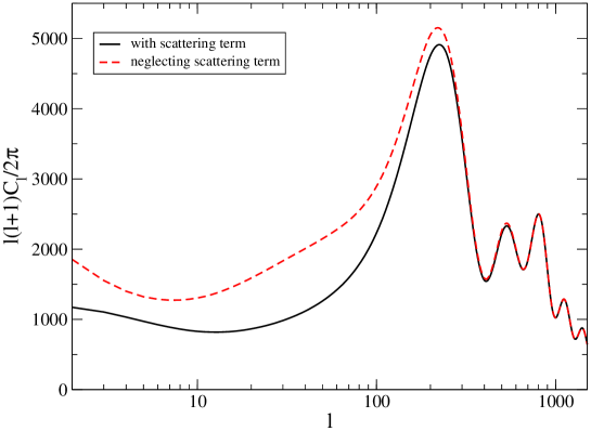
Figure 1: Differences between the CMB power spectra with and without the scattering term in the geodesic equation of neutrinos with the same cosmological parameters.

5 Quintessence potentials and Cosmological Constraints

To determine the evolution of scalar field which couples to neutrinos, we should specify the potential of the scalar field. A variety of quintessence effective potentials can be found in the literature. In the present paper we examine three type of quintessential potentials. First we analyze what is a frequently invoked form for the effective potential of the tracker field, i.e., an inverse power law originally analyzed by Ratra and Peebles [37],

$$V(\phi)=M^{4}\left({M_{pl}\over\phi}\right)^{\alpha}~{}~{}~{}\mbox{(Model I)}~{},$$ (54)

where $V_{0}=M^{4}=3M_{pl}^{2}H_{0}^{2}\Omega_{\phi}$ stands for the vacuum energy, $M_{pl}$ is the plank mass and $\alpha$ is free parameter which will be constrained from observational data.

We will also consider a modified form of $V(\phi)$ as proposed by [38] based on the condition that the quintessence fields be part of supergravity models. The potential now becomes

$$V(\phi)=M^{4}\left({M_{pl}\over\phi}\right)^{\alpha}e^{3\phi^{2}/2M_{\rm pl}^{2}}~{}~{}~{}\mbox{(Model II)}~{},$$ (55)

where the exponential correction becomes important near the present time as $\phi\to M_{\rm pl}$. The fact that this potential has a minimum for $\phi=\sqrt{\alpha/3}M_{\rm pl}$ changes the dynamics. It causes the present value of $w$ to evolve to a cosmological constant much quicker than for the bare power-law potential [39].

We will also analyze another class of tracking potential, namely, the potential of exponential type [40]:

$$V(\phi)=M^{4}e^{-\alpha({\phi\over M_{pl}})}~{}~{}~{}\mbox{(Model III)}~{},$$ (56)

This type of potential can lead to accelerating expansion provided that $\alpha<\sqrt{2}$. In figure (2), we present examples of evolution of energy densities with these three types of potentials with vanishing coupling strength to neutrinos.

Figure 2: Examples of the evolution of energy density in quintessence and the background fields as indicated. Model parameters taken to plot this figure are $\alpha=10$, $10$, $1$ for model I, II, III, respectively. The other parameters for the dark energy are fixed so that the energy densities in three types of dark energy should be the same at present.

5.1 Equation of State in Interacting Dark-Energy with Neutrinos

In quintessence models, the scalar field $\phi$ rolls down a self-interacting potential $V(\phi)$. The equation of state (EoS) is defined,

$$\omega_{\phi}={\dot{\phi}^{2}/2-V(\phi)\over\dot{\phi}^{2}/2+V(\phi)}.$$ (57)

It has to satisfy the condition $\omega_{\phi}<-1/3$ for the cosmic acceleration. Since $\omega_{\phi}\geq-1$ from eq.(57), the $\omega_{\phi}<-1$ regime can not be realized by quintessence. However observations have shown exciting possibility of $\omega_{\phi}<-1$, which causes the big-rip singularity problem by the phantom field at the end of the day. Various independent analysis of the Gold SN1a data set [41] indicated it. Present situations of the observation tell us: First cosmic shear results from the Canada-France-Hawaii Telescope (CFHT) Wide Synoptic Survey provided a constraint on a constant equation of state for dark-energy, based on cosmic shear data alone: $\omega_{0}<-0.8$ with $68\%$ C.L. from the Deep Component of the CFHTLS[42]. In the Supernova Legacy Survey (SNLS) [43] cosmological fits to the first year SNLS Hubble diagram gave $\omega=-1.023\pm 0.090\pm 0.054$ for a flat cosmology with constant equation of state when combined with the constraint from the recent Sloan Digital Sky Survey (SDSS) measurement of baryon acoustic oscillations. WMAP3 data [44] gave us two different results for different assumptions: when we assume flat universe including SNLS data, $\omega=-0.97^{+0.07}_{-0.09}$, however if we drop prior of flat universe, WMAP + LSS + SNLS data provide $\omega=-1.062^{+0.128}_{-0.079}$ and $\Omega_{k}=-0.024^{+0.016}_{-0.013}$. Still observations tell us the possibility of unexpected $\omega<-1$.

We summarize the possible values of EoS in various quintessence potential models in table 1.

Table 1: Equation of state in various quintessence potential models

Quintessence Potentials	Equation of State (EoS)	References
$M^{4}\,\,exp(-\lambda\phi)$	$\omega=\lambda^{2}/3-1$	Ratra & Peebles[45], Wetterich[46]
	$\lambda=\sqrt{3/\Omega_{\phi}}$, $\Omega_{\phi}<0.1-0.15$	Ferreira & Joyce[47]
$M^{4+\alpha}/\phi^{\alpha}$, $\alpha>0$	$\omega>-0.7$	Ratra & Peebles[45]
$M^{4}\,exp(\lambda\phi^{2})\,\phi^{-\alpha}$	$\alpha\geq 11$, $\omega\simeq-0.82$	Brax & Martin[48]
$m^{2}\phi^{2}$,   $\lambda\phi^{4}$	PNGB	Frieman et al.[49]
	$M^{4}\,[cos(\phi/f)+1]$
$M^{4}\,[exp(M_{pl}/\phi)-1]$	$\Omega_{m}>0.2$, $\omega<-0.8$	Zlatev, Wang & Steinhardt[50]
$M^{4}\,[cosh(\lambda\phi)-1]^{p}$	$p<1/2$, $\omega<-1/3$	Sahni & Wang[51]
$M^{4}\,sinh^{-\alpha}(\lambda\phi)$	early time: inverse power	Sahni & Starobinsky[52]
	late time: exponential	Urena-López & Matos[53]
$M^{4}\,[(\phi-B)^{\alpha}+A]\,exp{(-\lambda\phi)}$	$\omega\sim-1$	Albrecht & Skordis[54]
$M^{4}\,exp[\lambda(\phi/M_{pl})^{2}]$	$\omega\sim-1$	Lee, Olive & Pospelov[55]
$M^{4}\,cosh[\lambda\phi/M_{pl}]$	$\omega\sim-1$

In this section we show that $\omega_{\phi}<-1$ naturally arises when quintessence field interacts with neutrinos. Similar processes has been done before in the case of interacting dark-energy and dark-matter [16].

Figure 3: Time evolution of the effective equation of state parameter $w_{\rm eff}$ for models with potentials of inverse power law (Model I) and exponential types (Model III). The parameters are fixed to the best fitting values except for those shown in the figure. The effective equation of state parameter can be smaller than $-1$ at $z>0$.

As pointed out by earlier works it is possible to have the observational equation of state $w_{\rm eff}$ less than -1 in the neutrino-dark energy interacting models. The point is that any observer would unaware the dark energy interactions, and attribute any unusual evolution of neutrino energy density to that of dark energy. This is seen as follows. Let us consider the recent epoch where the neutrinos have already become massive enough so that the energy density of neutrinos can be described as

$$\rho_{\nu}=m_{\nu}(\phi)n_{\nu}=m_{\nu}(\phi)n_{\nu,0}/a^{3}~{},$$ (58)

where $n_{\nu},0$ is the number density of neutrinos at present time. One can decompose this into two parts as

$$\rho_{\nu}=m_{\nu}(\phi_{0})n_{\nu,0}/a^{3}+\left(\frac{m_{\nu}(\phi)}{m_{\nu}(\phi_{0})}-1\right)m_{\nu}(\phi_{0})n_{\nu,0}/a^{3}~{},$$ (59)

and hence the Friedmann equation (neglecting baryon and photon contributions)

$$H^{2} = \frac{8\pi G}{3}\left(\rho_{\rm CDM}+\rho_{\nu}+\rho_{\phi}\right)$$ (60)

$$= \frac{8\pi G}{3}\left(\left(\rho_{\rm CDM,0}+\rho_{\nu,0}\right)/a^{3}+\left(\frac{m_{\nu}(\phi)}{m_{\nu}(\phi_{0})}-1\right)m_{\nu}(\phi_{0})n_{\nu,0}/a^{3}+\rho_{\phi}\right)~{}.$$

Therefore, while the first term in the above equation is regarded as a (total) matter density of our universe, the second and third terms comprise effective energy density which would be recognized as dark energy,

$$\rho_{\rm eff}\equiv\left(\frac{m_{\nu}(\phi)}{m_{\nu}(\phi_{0})}-1\right)m_{\nu}(\phi_{0})n_{\nu,0}/a^{3}+\rho_{\phi}~{}.$$ (61)

In observations one measures the equation of state of dark energy $w_{\rm eff}$ defined by

$$\frac{d\rho_{\rm eff}}{dt}=-3H(1+w_{\rm eff})\rho_{\rm eff}~{}.$$ (62)

Here $w_{\rm eff}$ is related to the equation of state of quintessence $w_{\phi}$ through

$$w_{\rm eff} = \frac{w_{\phi}}{1-x}~{},$$ (63)

$$x = \left(\frac{m_{\nu}(\phi)}{m_{\nu}(\phi_{0})}-1\right)\frac{m_{\nu}(\phi_{0})n_{\nu,0}/a^{3}}{\rho_{\phi}}~{},$$ (64)

which are derived from Eqs.(3), (9), and (61). An example of time evolution of $w_{\rm eff}$ is depicted in Fig. (3).

5.2 Time evolution of neutrino mass and energy density in scalar field

For an illustration we also plot examples of evolution of energy densities for interacting case with inverse power law potential (Model I) in Fig. (4). In interacting dark energy cases, the evolution of the scalar field is determined both by its own potential and interacting term from neutrinos. When neutrinos are highly relativistic, the interaction term can be expressed as

$$(\rho_{\nu}-3P_{\nu})\approx\frac{10}{7\pi^{2}}(am_{\nu})^{2}\rho_{\nu_{\rm massless}}~{},$$ (65)

where $\rho_{\nu_{\rm massless}}$ denotes the energy density of neutrinos with no mass. The term roughly scales as $\propto a^{-2}$, and therefore, it dominates deep in the radiation dominated era. However, because the motion of the scalar field driven by this interaction term is almost suppressed by the friction term, $-2{\cal H}\dot{\phi}$. The scalar field satisfies the slow roll condition similar to the inflation models, $-2{\cal H}\dot{\phi}\approx a^{2}\frac{\partial m_{\nu}}{\partial\phi}(\rho_{\nu}-3P_{\nu})$. Thus, the energy density in scalar field and the mass of neutrinos is frozen there. These behaviors are clearly seen in Figs. (4) and (5). The derivation of the analytic expression for the behavior of varying neutrino mass in early time of the universe is given at Appendix B.

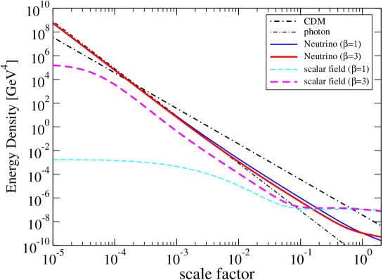
Figure 4: Examples of the evolution of energy density in quintessence and the background fields in coupled cases with inverse power law potential (Model I). Model parameters taken to plot this figure are $\alpha=1$, $\beta=1$, $3$ as indicated. The other parameters for the dark energy are fixed so that the energy densities in three types of dark energy should be the same at present.

Figure 5: Examples of the time evolution of neutrino mass in power law potential models (Model I) with $\alpha=1$ and $\beta=0$ (black solid line), $\beta=1$ (red dashed line), $\beta=2$ (blue dash-dotted line), $\beta=3$ (dash-dot-dotted line). The larger coupling parameter leads to the larger mass in the early universe.

5.3 Constrains on the MVN parameters and Neutrino Mass Bound

5.3.1 Neutrino Mass Bounds from Beta Decays and Large Scale Structures

In this section, we review in brief the present status of the determination of absolute neutrino mass from beta decay experiments and cosmological observation data. The existence of the tiny neutrino masses qualifies as the first evidence of new physics beyond the Standard Model. The answer to the hot questions on (1) whether neutrinos are Dirac or Majorana fermions ? (2) what kind of mass hierarchy pattern they have ? (3) what are the absolute values of the neutrino masses, will provide us the additional knowledge about the precise nature of this new physics, and in turn about the nature of new forces beyond the Standard Model. There are three well known ways to get the direct information on the absolute mass of neutrinos by using: Tritium $\beta$-decay experiment, neutrinoless double beta decay experiment, and astrophysical observations.

The standard method for the measurement of the absolute value of the neutrino mass is based on the detailed investigation of the high-energy part of the $\beta$-spectrum of the decay of tritium:

$${}^{3}H\longrightarrow{}^{3}He+e^{-}+\bar{\nu}_{e}$$ (66)

This decay has a small energy release ($E_{0}\simeq 18.6keV$) and a convenient life time ($T_{1/2}=12.3$ years). Since the flavor eigenstates are different from mass eigenstates in neutrino sector, in general, electron neutrino can be expressed as

$$\nu_{eL}=\sum_{i}U_{ei}\,\nu_{iL},$$ (67)

where $\nu_{i}$ is the field of neutrino with mass $m_{i}$, and U is the unitary mixing matrix. Neglecting the recoil of the final nucleus, the spectrum of the electrons is given:

$${d\Gamma\over dE}=\sum_{i}|U_{ei}|^{2}\,\,{d\Gamma_{i}\over dE},$$ (68)

and the resulting spectrum can be analyzed in term of a single mean-squared electron neutrino mass

$$\langle m_{\beta}\rangle^{2}=\sum_{j}m_{j}^{2}|U_{ej}|^{2}=m_{1}^{2}|U_{e1}|^{2}+m_{2}^{2}|U_{e2}|^{2}+m_{3}^{2}|U_{e3}|^{2}$$ (69)

If the neutrino mass spectrum is practically degenerate: $m_{1}\simeq m_{2}\simeq m_{3}$, the neutrino mass can be measured in these experiments. Present-day tritium experiments Mainz[56] and Troitsk[57] gave the following results:

$$m_{1}^{2} = (-1.2\pm 2.2\pm 2.1)\,eV^{2}\hskip 14.22636pt{\rm(Mainz)},$$ (70)

$$= (-2.3\pm 2.5\pm 2.0)\,eV^{2}\hskip 14.22636pt{\rm(Troitsk)}.$$ (71)

This value corresponds to the upper bound

$$m_{1}<\,2.2eV\hskip 8.53581pt(95\%C.L.)$$ (72)

Another useful method is by using the neutrinoless double beta decay. The search for neutrinoless double $\beta$-decay

$$(A,Z)\longrightarrow(A,Z_{2})+e^{-}+e^{-}$$ (73)

for some even-even nuclei is the most sensitive and direct way of investigating the nature of neutrinos with definite masses. In this process, total lepton number is violated and is allowed only if the massive neutrinos are Majorana particles. The rate of $0\nu\beta\beta$ is approximately

$${1\over T^{0\nu}_{1/2}}=G_{0\nu}(Q_{\beta\beta},Z)\,|M_{0\nu}|^{2}\,\,\langle m_{\beta\beta}\rangle^{2},$$ (74)

where $G^{0\nu}$ is the phase space factor for the emission of the two electrons, $M_{0\nu}$ is nuclear matrix elements, and $<m_{\beta\beta}>$ is the effective Majorana mass of the electron neutrino:

$$\langle m_{\beta\beta}\rangle\equiv|\sum_{i}U_{ei}^{2}m_{i}|$$ (75)

We can write eq.(75), for normal and inverted hierarchy respectively, in terms of mixing angles and $\Delta_{s}^{2}=m_{2}^{2}-m_{1}^{2}=7.9^{+2.8}_{-2.9}\cdot 10^{-5}\,eV^{2}$, $\Delta_{a}=\pm(m_{3}^{2}-m_{2}^{2})=\pm(2.6\pm 0.2)\cdot 10^{-3}\,eV^{2}$ at the $3\sigma$ level and CP phases as follows:

$$\langle m_{ee}\rangle = \left|c_{2}^{2}c_{3}^{2}m_{1}+c_{2}^{2}s_{3}^{2}e^{i\phi_{2}}\sqrt{\Delta_{s}^{2}+m_{1}^{2}}+s_{2}^{2}e^{i\phi_{3}}\sqrt{\Delta_{a}^{2}+m_{1}^{2}}\right|,\hskip 2.84526pt{\rm(normal\,\,hierarchy)}$$ (76)

$$\langle m_{ee}\rangle = \left|s_{2}^{2}m_{1}+c_{2}^{2}s_{3}^{2}e^{i\phi_{2}}\sqrt{\Delta_{a}^{2}-\Delta_{s}^{2}+m_{1}^{2}}+c_{2}^{2}s_{2}^{2}e^{i\phi_{3}}\right|,\hskip 17.07164pt{\rm(inverted\,\,hierarchy)}.$$ (77)

However, $0\nu\beta\beta$ decay have not yet been seen experimentally. The most stringent lower bounds for the life-time of $0\nu\beta\beta$-decay were obtained in the Heidelberg-Moscow[58] and IGEX[59] ${}^{76}Ge$ experiments:

$$T^{0\nu}_{1/2}\geq 1.9\cdot 10^{25}years\hskip 14.22636pt(90\%C.L.)\hskip 14.22636pt{\rm Heidelberg-Moscow},$$ (78)

$$T^{0\nu}_{1/2}\geq 1.57\cdot 10^{25}years\hskip 14.22636pt(90\%C.L.)\hskip 14.22636pt{\rm IGEX}.$$ (79)

Taking into account different calculation of the nuclear matrix elements, from these results the following upper bounds were obtained for the effective Majorana mass:

$$|m_{\beta\beta}|\,<\,(0.35-1.24)\,eV$$ (80)

Many new experiments (including CAMEO,CUORE,COBRA, EXO, GENIUS, MAJORANA, MOON and XMASS experiments) on the search for the neutrinoless double $\beta$-decay are in preparation at present. In these experiments the sensitivities

$$|m_{\beta\beta}|\simeq(0.1-0.015)\,eV$$ (81)

are expected to be achieved. More detail discussions will be appeared in the separated paper[60].

Within the standard cosmological model, the relic abundance of neutrinos at present epoch was come out straightforwardly from the fact that they follow the Fermi-Dirac distribution after freeze out, and their temperature is related to the CMB radiation temperature $T_{CMB}$ today by $T_{\nu}=(4/11)^{1/3}T_{CMB}$ with $T_{CMB}=2.726$ K, providing

$$n_{\nu}={6\zeta(3)\over 11\pi^{2}}\,T_{CMB}^{3},$$ (82)

where $\zeta(3)\simeq 1.202$, which gives $n_{\nu}\simeq 112cm^{-3}$ for each family of neutrinos at present. By now the massive neutrinos become non-relativistic, and their contribution to the mass density ($\Omega_{\nu}$) of the universe can be expressed as

$$\Omega_{\nu}h^{2}={\Sigma\over 93.14eV}.$$ (83)

where $\Sigma$ stands for the sum of the neutrino masses. In this relation, the effect of three neutrino oscillation is included [61]. We should notice that when obtaining the limit of neutrino masses one usually assumes:

• the standard spatially flat $\Lambda CDM$ model with adiabatic primordial perturbations,

• they have no non-standard interactions,

• neutrinos decoupled from the thermal background at the temperatures of order 1 MeV.

These simple conditions can be modified from several effects: due to a sizable neutrino-antineutrino asymmetry, due to additional light scalar field coupled with neutrinos [62], and due to the light sterile neutrino [63]. However, analysis of WMAP and 2dFGRS data gave independent evidence for small lepton asymmetries [64, 65], and such a scenario with a light scalar field is strongly disfavored by the current CMB power spectrum data [66]. We will not therefore take into account such non-standard couplings of neutrinos in the following. In addition, current cosmological observations are sensitive to neutrino masses $0.1\,{\rm eV}\,<\,\Sigma\,<\,2.0\,{\rm eV}$. In this mass scale, the mass-square differences are small enough and all three active neutrinos are nearly degenerate in mass. Therefore we take the assumption of degenerate mass hierarchy. Even if we consider different mass hierarchy pattern, it will be very difficult to distinguish such hierarchy patterns from cosmological data alone [67].

After neutrinos decoupled from the thermal background, they stream freely and their density perturbations are damped on scale smaller than their free streaming scale. Consequently the perturbations of cold dark matter (CDM) and baryons grow more slowly because of the missing gravitational contribution from neutrinos. The free streaming scale of relativistic neutrinos grows with the Hubble horizon. When the neutrinos become non-relativistic, their free streaming scale shrinks, and they fall back into the potential wells. The neutrino density perturbation with scales larger than the free streaming scale resumes to trace those of the other species. Thus the free streaming effect suppresses the power spectrum on scales smaller than the horizon when the neutrinos become non-relativistic. The co-moving wave number corresponding to this scale is given by

$$k_{nr}=0.026\,\left({m_{\nu}\over 1\,eV}\right)^{1/2}\,\Omega_{m}^{1/2}\,h\,{\rm Mpc}^{-1},$$ (84)

for degenerated neutrinos, with almost same mass $m_{\nu}$. The growth of Fourier modes with $k>k_{nr}$ will be suppressed because of neutrino free-streaming. The power spectrum of matter fluctuations can be written as

$$P_{m}(k,z)=P_{*}(k)\,T^{2}(k,z),$$ (85)

where $P_{*}(k)$ is the primordial spectrum of matter fluctuations, to be a simple power law $P_{*}(k)=A\,k^{n}$, where A is the amplitude and n is the spectral index. Here the transfer function $T(k,z)$ represents the evolution of perturbation relative to the largest scale. If some fraction of the matter density (e.g., neutrinos or dark energy) is unable to cluster, the speed of growth of perturbation becomes slower. Because the contribution to the fraction of matter density from neutrinos is proportional to their masses (Eq. (83)), the larger mass leads to the smaller growth of perturbation. The suppression of the power spectrum on small scales is roughly proportional to $f_{\nu}$ [68]:

$${\Delta P_{m}(k)\over P_{m}(k)}\simeq-8f_{\nu}.$$ (86)

where $f_{\nu}=\Omega_{\nu}/\Omega_{M}$ is the fractional contribution of neutrinos to the total matter density. This result can be understood qualitatively from the fact that only a fraction $(1-f_{\nu})$ of the matter can cluster when massive neutrinos are present [69].

Table 2: Recent cosmological neutrino mass bounds ($95\%$ C.L.)

Cosmological Data Set	$\Sigma$ bound ($2\sigma$)	References
CMB (WMAP-3 year alone)	$<\,2.0$ eV	Fukugita et al.[71]
LSS[2dFGRS]	$<\,1.8$ eV	Elgaroy et al.[72]
CMB + LSS[2dFGRS]	$<\,1.2$ eV	Sanchez et al.[73]
”	$<\,1.0$ eV	Hannestad[74]
CMB + LSS + SN1a	$<\,0.75$ eV	Barger et al.[75]
”	$<\,0.68$ eV	Spergel et al.[76]
CMB + LSS + SN1a + BAO	$<\,0.62$ eV	Goobar et al.[77]
”	$<\,0.58$ eV
CMB + LSS + SN1a + Ly-$\alpha$	$<\,0.21$ eV	Seljak et al.[6]
CMB + LSS + SN1a + BAO + Ly-$\alpha$	$<\,0.17$ eV	Seljak et al.[6]

Analyses of CMB data are not sensitive to neutrino masses if neutrinos behave as massless particles at the epoch of last scattering. According to the analytic consideration in [70], since the redshift when neutrino becomes non-relativistic is given by $1+z_{nr}=6.24\cdot 10^{4}\,\Omega_{\nu}\,h^{2}$ and $z_{rec}=1088$, neutrinos become non-relativistic before the last scattering when $\Omega_{\nu}h^{2}>0.017$ (i.e. $\Sigma>1.6eV$). Therefore the dependence of the position of the first peak and the height of the first peak on $\Omega_{\nu}h^{2}$ has a turning point at $\Omega_{\nu}h^{2}\simeq 0.017$. This value also affects CMB anisotropy via the modification of the integrated Sachs-Wolfe effect due to the massive neutrinos. However an important role of CMB data is to constrain other parameters that are degenerate with $\Sigma$. Also, since there is a range of scales common to the CMB and LSS experiments, CMB data provides an important constraint on the bias parameters. We summarize some of the recent cosmological neutrino mass bounds in table 2.

5.3.2 Neutrino Mass Bound in Neutrino-Dark Energy Model

As was shown in the previous sections, the coupling between cosmological neutrinos and dark energy quintessence could modify the CMB and matter power spectra significantly. It is therefore possible and also important to put constraints on coupling parameters from current observations. For this purpose, we use the WMAP3 [78, 79] and 2dFGRS [80] data sets. In figure 6, we demonstrate, as an example, the total neutrino mass contribution on the CMB angular power spectra with the inverse power law potential (Model 1). We can see that the deviations from observation data becomes severe when the total neutrino mass increases

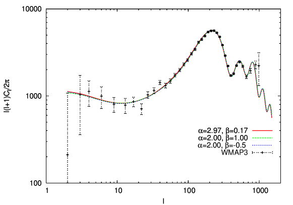
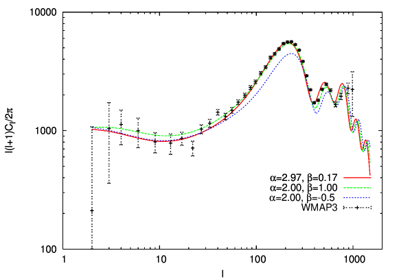
Figure 6: The CMB angular power spectra for Model I with different neutrino masses: $M_{\nu}=0.3$ eV (upper panel) and $M_{\nu}=1.0$ eV (down panel). The solid line is the best fit for the model ($(\alpha,\beta)=(2.97,0.170)$), the other lines are models with different parameter value of $\alpha$ and $\beta$ as indicated. The points are WMAP three year data.

The flux power spectrum of the Lyman-$\alpha$ forest can be used to measure the matter power spectrum at small scales around $z\mathrel{\mathchoice{\lower 3.6pt\vbox{\halign{$\mathsurround=0pt\displaystyle\hfil#\hfil$\cr<\crcr\sim\crcr}}}{\lower 3.6pt\vbox{\halign{$\mathsurround=0pt\textstyle\hfil#\hfil$\cr<\crcr\sim\crcr}}}{\lower 3.6pt\vbox{\halign{$\mathsurround=0pt\scriptstyle\hfil#\hfil$\cr<\crcr\sim\crcr}}}{\lower 3.6pt\vbox{\halign{$\mathsurround=0pt\scriptscriptstyle\hfil#\hfil$\cr<\crcr\sim\crcr}}}}3$ [81, 82]. It has been shown, however, that the resultant constraint on neutrino mass can vary significantly from $\sum m_{\nu}<0.2$eV to $0.4$eV depending on the specific Lyman-$\alpha$ analysis used [83]. The complication arises because the result suffers from the systematic uncertainty regarding to the model for the intergalactic physical effects, i.e., damping wings, ionizing radiation fluctuations, galactic winds, and so on [84]. Therefore, we conservatively omit the Lyman-$\alpha$ forest data from our analysis.

Because there are many other cosmological parameters than the MVN parameters, we follow the Markov Chain Monte Carlo(MCMC) global fit approach [85] to explore the likelihood space and marginalize over the nuisance parameters to obtain the constraint on parameter(s) we are interested in [86]. Our parameter space consists of

$$\vec{P}\equiv(\Omega_{b}h^{2},\Omega_{c}h^{2},H,\tau,A_{s},n_{s},m_{i},\alpha,\beta)~{},$$ (87)

where $\Omega_{b}h^{2}$ and $\Omega_{c}h^{2}$ are the baryon and CDM densities in units of critical density, $H$ is the Hubble parameter, $\tau$ is the optical depth of Compton scattering to the last scattering surface, $A_{s}$ and $n_{s}$ are the amplitude and spectral index of primordial density fluctuations, and $(m_{i},\alpha,\beta)$ are the parameters of MVN defined in section III. We have put priors on MVN parameters as $\alpha>0$, and $\beta>0$ for simplicity and saving the computational time.

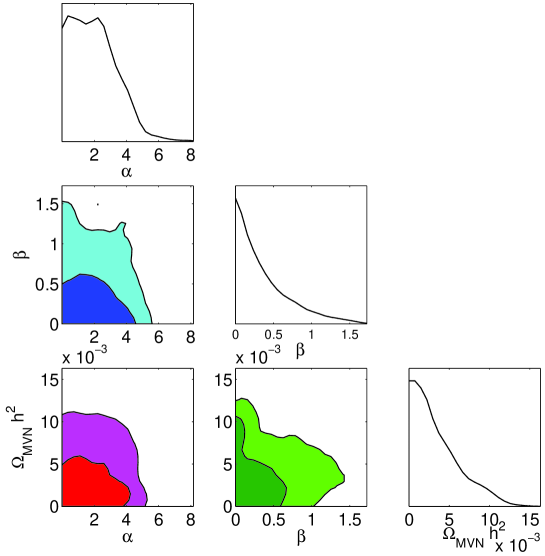
Figure 7: Contours of constant relative probabilities in two dimensional parameter planes for inverse power law models. Lines correspond to 68% and 95.4% confidence limits.

Figure 8: Same as Fig.(7), but for SUGRA type models.

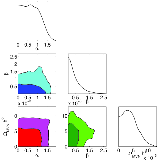
Figure 9: Same as Fig.(7), but for exponential type models.

Our results are shown in Figs.(7) - (9). In these figures we do not observe the strong degeneracy between the introduced parameters. This is why one can put tight constraints on MVN parameters from observations. For both models we consider, larger $\alpha$ leads larger $w$ at present. Therefore large $\alpha$ is not allowed due to the same reason that larger $w$ is not allowed from the current observations.

On the other hand, larger $\beta$ will generally lead larger $m_{\nu}$ in the early universe. This means that the effect of neutrinos on the density fluctuation of matter becomes larger leading to the larger damping of the power at small scales. A complication arise because the mass of neutrinos at the transition from the ultra-relativistic regime to the non-relativistic one is not a monotonic function of $\beta$ as shown in Fig.(5). Even so, the coupled neutrinos give larger decrement of small scale power, and therefore one can limit the coupling parameter from the large scale structure data.

One may wonder why we can get such a tight constraint on $\beta$, because it is naively expected that large $\beta$ value should be allowed if $\Omega_{\nu}h^{2}\sim 0$. In fact, a goodness of fit is still satisfactory with large $\beta$ value when $\Omega_{\nu}h^{2}\sim 0$. However, the parameters which give us the best goodness of fit does not mean the most likely parameters in general. In our parametrization, the accepted total volume by MCMC in the parameter space where $\Omega_{\nu}h^{2}\sim 0$ and $\beta\mathrel{\mathchoice{\lower 3.6pt\vbox{\halign{$\mathsurround=0pt\displaystyle\hfil#\hfil$\cr>\crcr\sim\crcr}}}{\lower 3.6pt\vbox{\halign{$\mathsurround=0pt\textstyle\hfil#\hfil$\cr>\crcr\sim\crcr}}}{\lower 3.6pt\vbox{\halign{$\mathsurround=0pt\scriptstyle\hfil#\hfil$\cr>\crcr\sim\crcr}}}{\lower 3.6pt\vbox{\halign{$\mathsurround=0pt\scriptscriptstyle\hfil#\hfil$\cr>\crcr\sim\crcr}}}}1$ was small, meaning that the probability of such a parameter set is low.

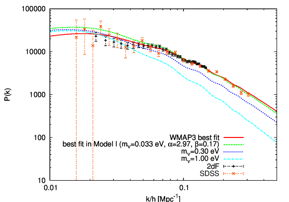
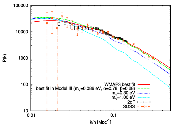
Figure 10: Examples of the total mass contributions in the matter power spectrum in Model I (upper panel) and Model III (down panel). For both panels we plot the best fitting lines (green dashed), lines with larger neutrino masses $M_{\nu}=0.3$ eV (blue dotted) and $M_{\nu}=1.0$ eV (cyan dot-dashed) with the other parameters fixed to the best fitting values. Note that while lines with $M_{\nu}=0.3$ eV can fit to the data well by arranging the other cosmological parameters, lines with $M_{\nu}=1.0$ eV can not.

In tables 3-5, we summerize our results of global analysis within $1\sigma$ and $2\sigma$ deviations for different types of quintessence potential with WMAP3 years data. We find no observational signature which favors the coupling between Mass Varying Neutrinos and quintessence scalar field, and obtain the upper limit on the coupling parameter as

$$\beta<0.46,0.47,0.58\,\,(1\,\sigma);\,\,[1.11,~{}1.36,~{}1.53\,\,(2\,\sigma)],$$ (88)

and the present mass of neutrinos is also limited to

$$\Omega_{\nu}h^{2}_{\rm{today}}<0.0044,~{}0.0048,~{}0.0048~{}\,\,(1\,\sigma);\,\,[0.0095,~{}0.0090,~{}0.0084~{}\,\,(2\,\sigma)],$$ (89)

for models I, II and III, respectively. When we apply the relation between the total sum of the neutrino masses $M_{\nu}$ and their contributions to the energy density of the universe: $\Omega_{\nu}h^{2}=M_{\nu}/(93.14eV)$, we obtain the constraint on the total neutrino mass: $M_{\nu}<0.45~{}eV(68\%C.L.)\,\,[0.87~{}eV(95\%C.L.)$] in the neutrino probe dark-energy model. The total neutrino mass contributions in the power spectrum is shown in Fig 10, where we can see the significant deviation from observation data in the case of large neutrino masses.

Before concluding the paper we should comment on the stability issue in the present models. As shown in [21, 22], some class of models with mass varying neutrinos suffers from the adiabatic instability at the first order perturbation level. This is caused by an additional force on neutrinos mediated by the quintessence scalar field and occurs when its effective mass is much larger than the Hubble horizon scale, where the effective mass is defined by $m_{\rm eff}^{2}={d^{2}V_{\rm eff}}/{d\phi^{2}}$. To remedy this situation one should consider an appropriate quintessential potential which has a mass comparable the horizon scale at present, and the models considered in this paper are the case [23]. Interestingly, some authors have found that one can construct viable MVN models by choosing certain couplings and/or quintessential potentials [87, 88, 89]. Some of these models even realises $m_{\rm eff}\gg H$. In Fig.(11), masses of the scalar field relative to the horizon scale $m_{\rm eff}/H$ are plotted. We find that $m_{\rm eff}<H$ for almost all period and the models are stable. We also depict in Fig.(11) the sound speed of neutrinos defined by $c^{2}_{s}=\delta P_{\nu}/\delta\rho_{\nu}$ with a wave number $k=2.3\times 10^{-3}$ Mpc^-1.

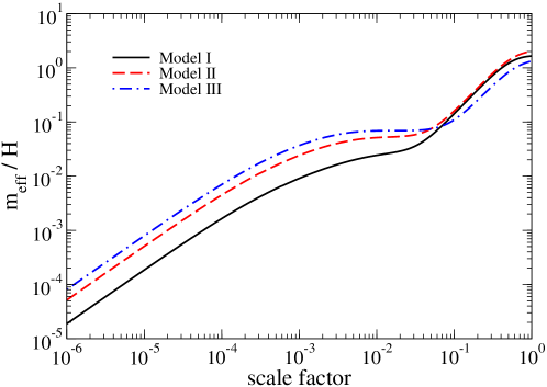
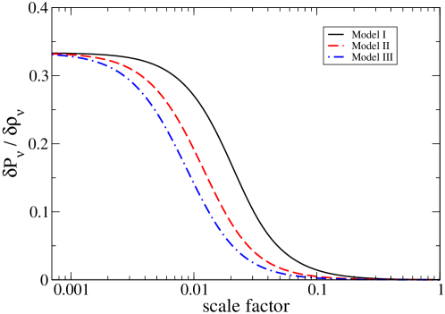
Figure 11: (upper panel): Typical evolution of the effective mass of the quintessence scalar field relative to the Hubble scale, for all models considered in this paper. (down panel): Typical evolution of the sound speed of neutrinos $c_{s}^{2}=\delta P_{\nu}/\delta\rho_{\nu}$ with the wave number $k=2.3\times 10^{-3}$ Mpc^-1, for models as indicated. The values stay positive stating from $1/3$ (relativistic) and neutrinos are stable against the density fluctuation.

Table 3: Global analysis data within $1\sigma$ and $2\sigma$ deviations for the inverse power law type (Model-I) of the quintessence potential. (*)Using WMAP data alone, they found 1.93, but along with either SDSS or 2dFGRS galaxy redshift data, they have 1.83 or 0.97 at $95\%$ confidence.

Quantites	Mean	SDDEV	$1\sigma$-ranges	$2\sigma$-ranges	WMAP3 data ($\Lambda$CDM)
$\alpha$	$2.08$	$1.35$	$<2.63$	$<4.38$	—
$\beta$	$0.38$	$0.35$	$<0.46$	$<1.12$	—
$\Omega_{B}\,h^{2}[10^{2}]$	$2.21$	$0.07$	$2.15-2.28$	$2.09-2.36$	$2.23\pm 0.07$
$\Omega_{CDM}\,h^{2}[10^{2}]$	$11.09$	$0.62$	$10.52-11.68$	$9.87-12.30$	$12.8\pm 0.8$
$H_{0}$	$65.97$	$3.61$	$62.30-69.37$	$58.39-72.10$	$72\pm 8$
$Z_{re}$	$10.87$	$2.58$	$9.81-12.15$	$6.13-14.94$	—
$n_{s}$	$0.95$	$0.02$	$0.94-0.97$	$0.92-0.99$	$0.958\pm 0.016$
$A_{s}[10^{10}]$	$20.66$	$1.31$	$19.38-21.92$	$18.25-23.41$	—-
$\Omega_{Q}[10^{2}]$	$68.54$	$4.81$	$64.02-72.94$	$57.43-75.60$	$71.6\pm 5.5$
$Age/Gyrs$	$13.95$	$0.20$	$13.76-14.15$	$13.59-14.40$	$13.73\pm 0.16$
$\Omega_{\nu}\,h^{2}[10^{2}]$	$0.36$	$0.29$	$<0.44$	$<0.95$	$<1.93(95\%C.L.)^{*}$
$\tau$	$0.084$	$0.029$	$0.055-0.112$	$0.031-0.143$	$0.089\pm 0.030$

Table 4: Global analysis data within $1\sigma$ and $2\sigma$ deviations for the SUGRA type (Model-II) of the quintessence potential.

Quantites	Mean	SDDEV	$1\sigma$-ranges	$2\sigma$-ranges	WMAP3 data ($\Lambda$CDM)
$\alpha$	$6.19$	$3.31$	$0.10-7.77$	$0.10-11.82$	—
$\beta$	$0.42$	$0.42$	$<0.47$	$<1.36$	—
$\Omega_{B}\,h^{2}[10^{2}]$	$2.22$	$0.07$	$2.16-2.29$	$2.09-2.35$	$2.23\pm 0.07$
$\Omega_{CDM}\,h^{2}[10^{2}]$	$11.10$	$0.65$	$10.47-11.75$	$9.85-12.40$	$12.8\pm 0.8$
$H_{0}$	$65.37$	$3.41$	$61.84-68.73$	$58.55-71.70$	$72\pm 8$
$Z_{re}$	$10.89$	$2.62$	$4.00-12.26$	$4.00-14.78$	—
$n_{s}$	$0.95$	$0.02$	$0.94-0.97$	$0.92-0.98$	$0.958\pm 0.016$
$A_{s}[10^{10}]$	$20.69$	$1.32$	$19.31-22.00$	$18.20-23.32$	—-
$\Omega_{Q}[10^{2}]$	$67.90$	$4.47$	$63.74-72.16$	$57.59-75.02$	$71.6\pm 5.5$
$Age/Gyrs$	$13.97$	$0.19$	$13.78-14.16$	$13.59-14.35$	$13.73\pm 0.16$
$\Omega_{\nu}\,h^{2}[10^{2}]$	$0.40$	$0.32$	$<0.48$	$<0.91$	$<1.93(95\%C.L.)$
$\tau$	$0.084$	$0.029$	$0.053-0.113$	$0.028-0.139$	$0.089\pm 0.030$

Table 5: Global analysis data within $1\sigma$ and $2\sigma$ deviations for the exponential type (Model-III) of the quintessence potential.

Quantites	Mean	SDDEV	$1\sigma$-ranges	$2\sigma$-ranges	WMAP3 data ($\Lambda$CDM)
$\alpha$	$0.70$	$0.42$	$<0.92$	$<1.41$	—
$\beta$	$0.50$	$0.48$	$<0.58$	$<1.53$	—
$\Omega_{B}\,h^{2}[10^{2}]$	$2.21$	$0.07$	$2.15-2.28$	$2.08-2.34$	$2.23\pm 0.07$
$\Omega_{CDM}\,h^{2}[10^{2}]$	$11.10$	$0.63$	$10.48-11.72$	$9.84-12.33$	$12.8\pm 0.8$
$H_{0}$	$65.61$	$3.26$	$62.37-68.70$	$58.99-71.58$	$72\pm 8$
$Z_{re}$	$11.07$	$2.44$	$10.07-12.35$	$6.64-14.78$	—
$n_{s}$	$0.95$	$0.02$	$0.94-0.97$	$0.92-0.98$	$0.958\pm 0.016$
$A_{s}[10^{10}]$	$20.73$	$1.24$	$19.48-21.95$	$18.33-23.27$	—-
$\Omega_{Q}[10^{2}]$	$68.22$	$4.17$	$64.38-72.08$	$58.45-75.05$	$71.6\pm 5.5$
$Age/Gyrs$	$13.96$	$0.19$	$13.77-14.15$	$13.61-14.36$	$13.73\pm 0.16$
$\Omega_{\nu}\,h^{2}[10^{2}]$	$0.38$	$0.25$	$<0.48$	$<0.84$	$<1.93(95\%C.L.)$
$\tau$	$0.086$	$0.027$	$0.058-0.113$	$0.032-0.140$	$0.089\pm 0.030$

6 Summary and conclusion:

In summary, we investigated the dynamics of dark energy in mass-varying neutrinos. We showed and discussed many aspects of the interacting dark-energy with neutrinos scenario: (1) To explain the present cosmological observation data, we don’t need to tune the coupling parameters between neutrinos and quintessence field, (2) Even with a inverse power law potential or exponential type potential which seem to be ruled out from the observation of $\omega$ value, we can receive that the apparent value of the equation of states can pushed down less than -1, (3) As a consequence of global fit, the cosmological neutrino mass bound beyond $\Lambda CDM$ model was first obtained with the value $\sum m_{\nu}<0.45\,eV(68\%C.L.)\,\,\,[0.87\,eV(95\%C.L.)]$.

Appendix A Boltzman Equations in Interacting Dark Energy-Neutrinos Scenario

From the Lagrangian ${\cal L}=-m(\phi)\sqrt{-g_{\mu\nu}\dot{x_{\mu}}\dot{x_{\nu}}}$, the Euler-Lagrange equation is given by

$${d\over d\lambda}\left(\partial{\cal L}\over\partial\dot{x}^{\mu}\right)={\partial{\cal L}\over\partial x^{\mu}}$$ (90)

where

$${\partial{\cal L}\over\partial\dot{x^{\mu}}} = P_{\mu}=m(x^{\mu})\,g_{\mu\alpha}{\dot{x}^{\alpha}\over\sqrt{-g_{\mu\nu}\dot{x}^{\mu}\dot{x}^{\nu}}},$$ (91)

$${\partial{\cal L}\over\partial x^{\mu}} = -{\partial m\over\partial x^{\mu}}\sqrt{-g_{\alpha\beta}\dot{x}^{\alpha}\dot{x}^{\beta}}+m(x^{\mu}){g_{\alpha\beta,\mu}\dot{x}^{\alpha}\dot{x}^{\beta}\over 2\sqrt{-g_{\alpha\beta}\dot{x}^{\alpha}\dot{x}^{\beta}}}$$ (92)

Therefore eq(90) becomes

$${1\over\sqrt{-g_{\alpha\beta}\dot{x}^{\alpha}\dot{x}^{\beta}}}{d\over d\lambda}\left(m(x^{\mu})\,{\dot{x}^{\mu}\over\sqrt{-g_{\alpha\beta}\dot{x}^{\alpha}\dot{x}^{\beta}}}\right)+{m(x^{\mu})\over 2}{g_{\alpha\beta,\mu}\dot{x}^{\alpha}\dot{x}^{\beta}\over g_{\alpha\beta}\dot{x}^{\alpha}\dot{x}^{\beta}}=-{\partial m\over\partial x^{\mu}}$$ (93)

By using the relation $ds=\sqrt{-g_{\alpha\beta}\dot{x}^{\mu}\dot{x}^{\nu}}d\lambda$, we obtain

$$P^{\mu}=m(x^{\mu}){\dot{x}^{\mu}\over\sqrt{-g_{\alpha\beta}\dot{x}^{\alpha}\dot{x}^{\beta}}}=m(x^{\mu}){dx^{\mu}\over ds}$$ (94)

and eq.(93) becomes

$${d\over ds}\left(m(x^{\mu})g_{\mu\beta}{dx^{\beta}\over ds}\right)-{m(x^{\mu})\over 2}g_{\alpha\beta,\mu}{dx^{\alpha}\over ds}{dx^{\beta}\over ds} = -{\partial m\over\partial x^{\mu}},$$ (95)

$${d\over ds}(g_{\mu\beta}P^{\beta})-{1\over 2}g_{\alpha\beta,\mu}P^{\alpha}{dx^{\beta}\over ds} = -{\partial m\over\partial x^{\mu}}$$ (97)

With simple calculation, finally we obtain the relations:

$${dP^{\nu}\over ds}+\Gamma^{\nu}_{\alpha\beta}\,P^{\alpha}{dx^{\beta}\over ds} = -g^{\nu\mu}{\partial m\over\partial x^{\mu}}$$ (98)

$$P^{0}{dP^{\nu}\over d\tau}+\Gamma^{\nu}_{\alpha\beta}\,P^{\alpha}P^{\beta} = -mg^{\nu\mu}m_{,\nu}.$$ (99)

For $\mu=0$ component, eq.(99) can be expressed as

$${1\over 2}{d\over d\tau}(P^{0})^{2}+\Gamma^{0}_{\alpha\beta}\,P^{\alpha}P^{\beta}=-mg^{0\mu}m_{,\mu}.$$ (100)

Since $P^{0}=g^{00}P_{0}=a^{-2}\epsilon$, each terms of the eq.(100) are given by:

$${\rm First\,\,term} = -2a^{-4}Hq^{2}+a^{-4}q{dq\over d\tau}-a^{-2}Hm^{2}+a^{-2}m{dm\over d\tau}$$ (101)

$${\rm Second\,\,term} = 2a^{-4}Hq^{2}+a^{-2}Hm^{2}+a^{-4}{1\over 2}\dot{h}_{ij}q^{i}q^{j}$$ (102)

$${\rm Third\,\,term} = a^{-2}m{\partial m\over\partial\tau}$$ (103)

Since the first term includes the total derivative w.r.t. comoving time, we obtain finally the eq.(42) in Section III-C:

$${dq\over d\tau}=-{1\over 2}\dot{h}_{ij}\,q\,n^{i}n^{j}-a^{2}{m\over q}{\partial m\over\partial x^{i}}\,{dx^{i}\over d\tau}.$$ (104)

Appendix B Varying Neutrino Mass in Early stage of Universe

In the high-redshift region with $z>100$, neutrinos behavior as like relativistic particles, even though they have non-zero mass. Since $1/\epsilon=[1-a^{2}m^{2}/2\,q^{2}]/q$ we have

$$(\rho-3P_{\nu}) = a^{-4}\int{d^{3}q\over(2\pi)^{3}}{a^{2}m^{2}\over\epsilon}\,f_{0},$$ (105)

$$= {a^{-4}\over(2\pi)^{2}}[\int q\,dq\,(a\,m)^{2}\,f_{0}-\int{dq\over q}(a\,m)^{4}\,f_{0}],$$

$$= {a^{-4}\over(2\pi)^{2}}[{\pi^{2}\over 12}(a\,m)^{2}-{\cal O}(a^{4}\,m^{4})]$$

For the massless neutrino case, the energy density is govern by

$$(\rho_{\nu})_{massless}=a^{-4}\int{d^{3}q\over(2\pi)^{3}}\,\,q\,\,f_{0}={a^{-4}\over(2\pi)^{2}}{7\over 120}\pi^{4}.$$ (106)

Then when we normalize it w.r.t. the energy density of massless neutrino:

$${(\rho_{\nu}-3\,P_{\nu})\over(\rho_{\nu})_{massless}}={10\over 7\,\pi^{2}}(a\,m)^{2}$$ (107)

Now we solve the equation of motion of quintessence field from eq.(3)with exponential type potential (Model III) for simplicity:

$$\ddot{\phi}+2{\cal H}\dot{\phi} = -a^{2}{dV\over d\phi}-a^{2}{dV_{I}\over d\phi}$$ (108)

$$= a^{2}\alpha\,V(\phi)-a^{2}{\beta\over M_{pl}}(\rho_{\nu}-3\,P_{\nu})$$

In the relativistic neutrino case when they obey the slow-rolling condition:

$$2{\cal H}\dot{\phi}\approx-a\,\,{\beta\over M_{pl}}\,\,(\rho_{\nu}-3\,P_{\nu})\propto-\beta$$ (109)

Since the relative sign of $\beta$ and $\phi$ is always opposite, the slope of the varying neutrino mass become negative, this means that the primordial neutrino mass was decreasing when universe was expanded.

Appendix C Consistency check

The form of $\kappa$ can be also obtained by demanding conservations of energy and momentum, i.e., demanding that $\nabla_{\mu}\stackrel{{\scriptstyle\mbox{\tiny($\phi$)}}}{{\delta T^{\mu}_{\nu}}}+\nabla_{\mu}\stackrel{{\scriptstyle\mbox{\tiny($\nu$)}}}{{\delta T^{\mu}_{\nu}}}~{}=~{}0$. Let us begin by considering the divergence of the perturbed stress-energy tensor for the scalar field,

$$\nabla_{\mu}\stackrel{{\scriptstyle\mbox{\tiny($\phi$)}}}{{\delta T^{\mu}_{\nu}}} = -a^{-2}\left(\ddot{\phi}+2{\cal H}\dot{\phi}+a^{2}\frac{dV}{d\phi}\right)\partial_{\nu}\delta\phi-a^{-2}\left(\ddot{\delta\phi}+2{\cal H}\dot{\delta\phi}+k^{2}\delta\phi+a^{2}\frac{d^{2}V}{d\phi^{2}}\right)\partial_{\nu}\phi$$ (110)

$$= \delta\left(\frac{dV_{I}}{d\phi}\right)\partial_{\nu}{\phi}+\frac{dV_{I}}{d\phi}\partial_{\nu}{\delta\phi}$$

where in the last line we used eqs.(3) and (19). The divergence of the perturbed stress-energy tensor for the neutrinos is given by,

$$\nabla_{\mu}\stackrel{{\scriptstyle\mbox{\tiny($\nu$)}}}{{\delta T^{\mu}_{0}}}=-\dot{\delta\rho}-(\rho+P)\partial_{i}v_{i}-3{\cal H}(\delta\rho+\delta P)-\frac{1}{2}\dot{h}(\rho+P)$$ (111)

for the time component and

$$\nabla_{\mu}\stackrel{{\scriptstyle\mbox{\tiny($\nu$)}}}{{\delta T^{\mu}_{i}}}=(\rho+P)\dot{v_{i}}+(\dot{\rho}+\dot{P})v_{i}+4{\cal H}(\rho+P)v_{i}+\partial_{i}P+\partial_{j}\Sigma^{j}_{i}$$ (112)

for the spatial component. Let us check the energy flux conservation for example, starting with the energy flux in neutrinos (in $k$-space):

$$(\rho_{\nu}+P_{\nu})\theta_{\nu}=4\pi ka^{-4}\int q^{2}dqqf_{0}(q)\Psi_{1}$$ (113)

where $\theta_{\nu}=ik^{i}v_{\nu~{}i}$. Differentiate with respect to $\tau$, we obtain,

$$(\rho_{\nu}+P_{\nu})\dot{\theta}_{\nu}+(\dot{\rho}_{\nu}+\dot{P}_{\nu})\theta_{\nu} = 4\pi ka^{-4}\int q^{2}dqqf_{0}\dot{\Psi}_{1}-4{\cal H}(\rho_{\nu}+P_{\nu})\theta_{\nu}$$ (114)

Let us consider the first term in the right hand side of the above equation. This gives

$$4\pi ka^{-4}\int q^{2}dqqf_{0}\dot{\Psi}_{1} = 4\pi ka^{-4}\int q^{2}dqqf_{0}\left[\frac{1}{3}\frac{q}{\epsilon}k(\Psi_{0}-2\Psi_{2})+\kappa\right]$$

$$= k^{2}\delta P_{\nu}-k^{2}(\rho_{\nu}+P_{\nu})\sigma_{\nu}+\frac{1}{3}4\pi k^{2}a^{-4}\int q^{2}dq\frac{q^{2}}{\epsilon^{2}}\frac{\partial\epsilon}{\partial\phi}\delta\phi f_{0}$$

$$+4\pi ka^{-4}\int q^{2}dqqf_{0}\kappa$$

where $\sigma$ is defined as $(\rho+P)\sigma=-(k_{i}k_{j}-\frac{1}{3}\delta_{ij})\Sigma^{i}_{j}$ and expressed by the distribution function as

$$(\rho_{\nu}+P_{\nu})\sigma_{\nu}=\frac{8\pi}{3}a^{-4}\int q^{2}dq\frac{q^{2}}{\epsilon}f_{0}(q)\Psi_{2}$$ (115)

Comparing eq. (114) with eq.(112), we find that the divergence of the perturbed stress-energy tensor in spatial part for the neutrinos leads to

$$\partial^{i}\nabla_{\mu}\stackrel{{\scriptstyle\mbox{\tiny($\nu$)}}}{{\delta T^{\mu}_{i}}}=\frac{1}{3}4\pi k^{2}a^{-4}\int q^{2}dq\frac{q^{2}}{\epsilon^{2}}\frac{\partial\epsilon}{\partial\phi}\delta\phi f_{0}+4\pi ka^{-4}\int q^{2}dqqf_{0}\kappa$$ (116)

On the other hand, the divergence of the perturbed stress-energy tensor in spatial part for scalar field is, from eq.(110),

$$\partial^{i}\nabla_{\mu}\stackrel{{\scriptstyle\mbox{\tiny($\phi$)}}}{{\delta T^{\mu}_{i}}} = -k^{2}\delta\phi\left(\frac{\partial\ln m_{\nu}}{\partial\phi}\right)(\rho_{\nu}-3P_{\nu})=-4\pi k^{2}\delta\phi a^{-4}\int q^{2}dq\frac{\partial\epsilon}{\partial\phi}f_{0}~{}.$$ (117)

These two equations imply that $\kappa$ shold take the form as eq. (52).

Next let us check the energy conservation. Density perturbation in neutrino is, (see eq.(28))

$$\delta\rho_{\nu}=a^{-4}\int\frac{d^{3}q}{(2\pi)^{3}}\epsilon f_{0}(q)\Psi_{0}+a^{-4}\int\frac{d^{3}q}{(2\pi)^{3}}\frac{\partial\epsilon}{\partial\phi}\delta\phi f_{0}~{},$$ (118)

By differenciate with respect to $\tau$, we obtain

$$\delta\dot{\rho}_{\nu} = -4{\cal H}\delta\rho_{\nu}+a^{-4}\int\frac{d^{3}q}{(2\pi)^{3}}\dot{\epsilon}f_{0}\Psi_{0}+a^{-4}\int\frac{d^{3}q}{(2\pi)^{3}}\epsilon f_{0}\dot{\Psi}_{0}$$ (119)

$$+a^{-4}\int\frac{d^{3}q}{(2\pi)^{3}}\frac{\partial}{\partial\tau}\left(\frac{\partial\epsilon}{\partial\phi}\right)\delta\phi f_{0}+a^{-4}\int\frac{d^{3}q}{(2\pi)^{3}}\frac{\partial\epsilon}{\partial\phi}\dot{\delta\phi}f_{0}$$

where

$$\dot{\epsilon} = ({\cal H}a^{2}m^{2}+a^{2}m^{2}\frac{\partial\ln m_{\nu}}{\partial\phi}\dot{\phi})/\epsilon~{},$$

$$\frac{\partial}{\partial\tau}\left(\frac{\partial\epsilon}{\partial\phi}\right) = -{\cal H}\frac{a^{2}m^{2}}{\epsilon^{2}}\frac{\partial\epsilon}{\partial\phi}+2{\cal H}\frac{\partial\epsilon}{\partial\phi}+\frac{\partial^{2}\epsilon}{\partial\phi^{2}}\dot{\phi}$$ (120)

Inserting eq.(48) for $\dot{\Psi}_{0}$ in the above equation, we obtain

$$\delta\dot{\rho}_{\nu} = -3{\cal H}(\delta\rho_{\nu}+\delta P_{\nu})-(\rho_{\nu}+P_{\nu})\theta_{\nu}-\frac{1}{2}\dot{h}(\rho_{\nu}+P_{\nu})$$ (121)

$$+a^{-4}\int\frac{d^{3}q}{(2\pi)^{3}}f_{0}\left(\frac{\partial^{2}\epsilon}{\partial\phi^{2}}\delta\phi+\Psi_{0}\frac{\partial\epsilon}{\partial\phi}\right)\dot{\phi}+a^{-4}\int\frac{d^{3}q}{(2\pi)^{3}}f_{0}\frac{\partial\epsilon}{\partial\phi}\dot{\delta\phi}$$

Comparing with eq.(111), we find

$$\nabla_{\mu}\stackrel{{\scriptstyle\mbox{\tiny($\nu$)}}}{{\delta T^{\mu}_{0}}}=-a^{-4}\int\frac{d^{3}q}{(2\pi)^{3}}f_{0}\left(\frac{\partial^{2}\epsilon}{\partial\phi^{2}}\delta\phi+\Psi_{0}\frac{\partial\epsilon}{\partial\phi}\right)\dot{\phi}-a^{-4}\int\frac{d^{3}q}{(2\pi)^{3}}f_{0}\frac{\partial\epsilon}{\partial\phi}\dot{\delta\phi}~{},$$ (122)

which is found to be equal to $-\nabla_{\mu}\stackrel{{\scriptstyle\mbox{\tiny($\phi$)}}}{{\delta T^{\mu}_{0}}}=-\delta\left(\frac{dV_{I}}{d\phi}\right)\dot{\phi}-\frac{dV_{I}}{d\phi}\delta\dot{\phi}$.

Acknowledgements:
We would like to thank L. Amendola, S. Carroll, T. Kajino, Lily Schrempp and O. Seto for useful comments and exciting discussions. K.I. thanks C. van de Bruck for useful communications. K.I.’s work is supported by Grant-in-Aid for JSPS Fellows. Y.Y.K’s work is partially supported by Grants-in-Aid for NSC in Taiwan, and Center for High Energy Physics(CHEP)/KNU and APCTP/Pohang in Korea. K.I. thanks KICP and National Taiwan university for kind hospitality where some parts of this work has been done. Y.Y. K. also thanks T. Kajino and NAOJ in Japan for kind hospitality where some parts of this work has been done.

References

- [1] S. Perlmutter et al.,Nature 391 (1998) 51[arXiv:astro-ph/7912212]; A. G. Riess et al., Astrophys. J. 116 (1998) 1009[arXiv:astro-ph/980520]; S. Perlmutter et al., ApJ 517 (1999) 565[arXiv:astro-ph/9812133].
- [2] C. L. Bennett et al., Astrophys. J. Suppl. Ser. 148 (2003) 1; J. L. Tonry et al.,Astrophys. J. 594 (2003) 1; M. Tegmark et al., Astrophys. J. 606 (2004) 702.
- [3] L. M. Krauss and M. S. Turner, Gen. Rel. Grav. 27 (1995) 1137 ; P. J. E. Peebles and B. Ratra, Reviews of Modern Physics, Vol75 (2003) 559.
- [4] C. Wetterich, Nucl. Phys. B302 (1988) 645.
- [5] S. M. Carroll, M. Trodden and M. S. Turner, Phys. Rev. D70: 043528 (2004).
- [6] U. Seljak, A. Slosar, and P. McDonald, J. Cosmol Astropart. Phys. 10 (2006) 014.
- [7] W. J. Percival, S. Cole, D. J. Eisenstein, R. C. Nichol, J. A. Peacock, A. C. Pope and A. S. Szalay, Mon. Not. Roy. Astron. Soc. 381, 1053 (2007) [arXiv:0705.3323 [astro-ph]].
- [8] R. G. Crittenden and N. Turok, Phys. Rev. Lett. 76, 575 (1996) [arXiv:astro-ph/9510072].
- [9] W. Hu and R. Scranton, Phys. Rev. D 70, 123002 (2004) [arXiv:astro-ph/0408456].
- [10] M. Takada, Phys. Rev. D 74, 043505 (2006) [arXiv:astro-ph/0606533].
- [11] S. Hannestad, Phys. Rev. D 71, 103519 (2005) [arXiv:astro-ph/0504017].
- [12] K. Ichiki and T. Takahashi, Phys. Rev. D 75, 123002 (2007) [arXiv:astro-ph/0703549].
- [13] S. M. Carroll, Phys. Rev. Lett. 81, 3067 (1998) [arXiv:astro-ph/9806099].
- [14] R. Bean and J. Magueijo, Phys. Lett. B 517, 177 (2001) [arXiv:astro-ph/0007199].
- [15] G. R. Farrar and P. J. E. Peebles, Astrophys. J. 604, 1 (2004) [arXiv:astro-ph/0307316].
- [16] S. Das, P. S. Corasaniti and J. Khoury, Phys. Rev. D 73, 083509 (2006).
- [17] S. Lee, G. C. Liu and K. W. Ng, Phys. Rev. D 73, 083516 (2006) [arXiv:astro-ph/0601333].
- [18] G. C. Liu, S. Lee and K. W. Ng, Phys. Rev. Lett. 97, 161303 (2006) [arXiv:astro-ph/0606248].
- [19] R. Fardon, A. E. Nelson and N. Weiner, JCAP 0410:005, 2004; [arXiv:astro-ph/0309800].
- [20] D. B. Kaplan, A. E. Nelson and N. Weiner, Phys. Rev. Lett. 93:091801, (2004); R. D. Peccei, Phys. Rev. D71:023527 (2005).
- [21] N. Afshordi, M. Zaldarriaga and K. Kohri, Phys. Rev. D 72, 065024 (2005) [arXiv:astro-ph/0506663].
- [22] R. Bean, E. E. Flanagan and M. Trodden, arXiv:0709.1128 [astro-ph].
- [23] A. W. Brookfield, C. van de Bruck, D. F. Mota, and D. Tocchini-Valentini, Phys. Rev. Lett , 96: 061301,2006; Phys. Rev. D73:083515,2006.
- [24] G. B. Zhao, J. Q. Xia and X. M. Zhang, arXiv:astro-ph/0611227.
- [25] A. W. Brookfield, C. van de Bruck, D. F. Mota and D. Tocchini-Valentini, Phys. Rev. D 76, 049901 (2007)
- [26] G. R. Dvali, G. Gabadadze and M. Porrati, Phys. Lett. B 485, 208 (2000) [arXiv:hep-th/0005016].
- [27] P. Binétruy, C. Deffayet, U. Ellwanger and D. Langlois, Phys. Lett. B 477 (2000) 285; P. Binétruy, C. Deffayet and D. Langlois, Nucl. Phys. B 565 (2000) 269; For a review of Brane World Cosmology, P. Brax, C. van de Bruck and A. C. Davis, Rept. Prog. Phys. 67:2183-2232 (2004).
- [28] J. D. Bekenstein, Phys. Rev. D70:083509 (2004); Erratum-ibid. D71:069901 (2005); C. Skordis, D. F. Mota, P. G. Ferreira and C. Boehm, Phys. Rev. Lett. 96:011301 (2006).
- [29] E. J. Copeland, M. Sami, and S. Tsujikawa, Int. J. Mod. Phys., D15: 1753 (2006).
- [30] T. Chiba, T. Okabe, M. Yamaguchi, Phys. Rev. D62: 023511, 2000.
- [31] C. A. Picon, V. F.Mukhanov, P. J. Steinhardt, Phys. Rev. D63: 103510, 2001.
- [32] R. R. Caildwell, Phys. Lett. B 545: 23, (2002).
- [33] Z. K. Guo,Y.-S. Piao, X.-M. Zhang and Y.-Z Zhang, Phys. Lett. B 608, 177 (2005).
- [34] X. J. Bi, P. h. Gu, X. l. Wang and X. M. Zhang, Phys. Rev. D69:113007 (2004); [arXiv:hep-ph/0311022].
- [35] C. P. Ma and E. Bertschinger, Astrophys. J. 455, 7 (1995).
- [36] G. W. Anderson and S. M. Carroll, arXiv:astro-ph/9711288.
- [37] B. Ratra and P. J. E. Peebles, Phys. Rev. D 37, 3406 (1988).
- [38] P. Brax and J. Martin, Phys. Lett. B 468, 40 (1999) [arXiv:astro-ph/9905040].
- [39] P. Brax, J. Martin and A. Riazuelo, Phys. Rev. D 62, 103505 (2000) [arXiv:astro-ph/0005428]. [40]
- [40] E. J. Copeland, A. R. Liddle and D. Wands, Phys. Rev. D 57, 4686 (1998) [arXiv:gr-qc/9711068].
- [41] A. G. Riess et al., Astrophys. J. 607, 665 (2004).
- [42] H. Hoekstra et al. [CFHT collaboration], arXiv:astro-ph/0511089, 2005.
- [43] P. Astier et al. [SNLS collaboration], Astron. Astrophy. 447 (2006) 31[astro-ph/0510447].
- [44] D. Spergel at al. [WMAP collaboration], Astrophys. J. Suppl. 170 (2007) 377 [astro-ph/0603449].
- [45] B. Ratra and P. J.E. Peebles, Astrophys. J. Lett. 325 (1988) 17; Phys. Rev. D 37 3406(1988).
- [46] C. Wetterich, Nucl. Phys. B302 (1988) 645.
- [47] P. G Ferreira and M. Joyce, Phys. Rev. Lett79 4740 (1997)
- [48] P. Brax and J. Martin, Phys. Lett. B468 (1999) 40.
- [49] J. A. Frieman, C. T. Hill, A.Stebbins and I. Waga, Phys. Rev. Lett75 2077 (1995).
- [50] I. Zlatev, L.-M. Wang and P. J. Steinhardt, Phys. Rev. Lett82 896 (1999).
- [51] V. Sahni and L.-M. Wang, Phys. Rev. D62 (2000) 103517.
- [52] V. Sahni and A. A. Starobinsky, Int. J. Mod. Phys. D9 373 (2000).
- [53] L. A. Urena-Lopez and T. Matos, Phys. Rev. D62 081302 (2000).
- [54] A. Albrecht and C. Skordis, Phys. Rev. Lett84 2076 (2000).
- [55] S. Lee, K. A. Olive and M. Pospelov, Phys. Rev. D70 083503 (2004).
- [56] J.Bonne et al., Nuch. Phys. B (Proc. Suppl.), 91 (2001) 273.
- [57] Ch. Weinheimer, Nucl. Phys. B (Proc. Suppl.), 118 (2003) 279.
- [58] L. Baudis et al. [Heidelberg-Moscow Collaboration], Phys. Rev. Lett. 83, 41 (1999).
- [59] C. E. Aalseth et al. [IGEX Collaboration], Phys. Rev. D 65, 092007 (2002); Phys. Rev. D 70, 078302 (2004).
- [60] Y.-Y. Keum, K. Ichiki and T. Kajino, ”Neutrino Mass Bounds from the Decays and Large Scale Structures”, Presented at the 10th International Symposium on Origin of Matter and Evolution of Galaxies, Dec. 4-7, 2007, Sapporo, Japan; arXiv:0803.2393; Yong-Yeon Keum, K. Ichiki, T. Kajino and G. J. Mathews, ”Neutrino mass bounds from Neutrinoless Double Beta Decays and Cosmological Probes including Ly- data”, in preparation.
- [61] G. Mangano et al., Nucl. Phys. B729 (2005) 221.
- [62] J. F. Beacom, N. F. Bell and S. Dodelson, Phys. Rev. Lett. 93 121302 (2004).
- [63] S. Dodelson, A. Melchiorri and A. Slasar, Phys. Rev. Lett. 97 04031 (2006).
- [64] S. Hannestad, JCAP 05 004 (2003).
- [65] E. Pierpaoli, Mon. Not. Roy. Astron. Soc. 342 L63 (2003).
- [66] S. Hannestad, JCAP 0502 011 (2005); arXiv astro-ph/0411475.
- [67] A Slosar, Phys. Rev. D73 123501 (2006).
- [68] W. Hu, D. J. Eisenstein and M. Tegmark, Phys. Rev. Lett. 80, 5255 (1998) [arXiv:astro-ph/9712057].
- [69] J. R. Bond, G. Efstathiou and J. Silk, Phys. Rev. Lett. 45 1980 (1980).
- [70] K. Ichikawa, M. Fukugita and M. Kawasaki, Phys. Rev. D71 043001 (2005).
- [71] M. Fukugita, K. Ichikawa, M. Kawasaki and O, Lahav, Phys. Rev. D 74, 027302 (2006).
- [72] O. Elgaroy et al., Phys. Rev. Lett89 061310 (2002); O. Elgaroy and O. Lahav, JCAP 0304 (2003) 004.
- [73] A. G. Sanchez et al., Mon. Not. Roy. Astron. Soc. 366 (2006) 189.
- [74] S. Hannestad, JCAP 0305 (2003) 004.
- [75] V. Barger, D. Marfatia, and A. Tregre, Phys. Lett. B 595 55 (2004).
- [76] D. N. Spergel et al. [WMAP Collaboration], astro-ph/0603449.
- [77] A. Goodbar, S. Hannestad, E. Mortsell, and H. Tu, J. Cosmol. Astropart. Phys. 06 (2006) 019.
- [78] G. Hinshaw et al.(WMAP collaboration), arXiv:astro-ph/0603451.
- [79] L. Page et al.(WMAP collaboration), arXiv:astro-ph/0603450.
- [80] S. Cole et al. [The 2dFGRS Collaboration], Mon. Not. Roy. Astron. Soc. 362, 505 (2005) [arXiv:astro-ph/0501174].
- [81] P. McDonald, J. Miralda-Escude, M. Rauch, W. L. W. Sargent, T. A. Barlow, R. Cen and J. P. Ostriker, Astrophys. J. 543, 1 (2000) [arXiv:astro-ph/9911196].
- [82] R. A. C. Croft et al., Astrophys. J. 581, 20 (2002) [arXiv:astro-ph/0012324].
- [83] A. Goobar, S. Hannestad, E. Mortsell and H. Tu, JCAP 0606, 019 (2006) [arXiv:astro-ph/0602155].
- [84] P. McDonald, U. Seljak, R. Cen, P. Bode and J. P. Ostriker, Mon. Not. Roy. Astron. Soc. 360, 1471 (2005) [arXiv:astro-ph/0407378].
- [85] A. Lewis and S. Bridle, Phys. Rev. D66, 103511 (2002).
- [86] Some useful comments of the numerical analysis code for the mass-varying neutrinos can be found in S. Goswami et al., Pramana 63:1391-1406(2004);[arXiv:hep-ph/0409225].
- [87] O. E. Bjaelde, A. W. Brookfield, C. van de Bruck, S. Hannestad, D. F. Mota, L. Schrempp and D. Tocchini-Valentini, arXiv:0705.2018 [astro-ph].
- [88] M. Kaplinghat and A. Rajaraman, Phys. Rev. D 75, 103504 (2007) [arXiv:astro-ph/0601517].
- [89] R. Takahashi and M. Tanimoto, JHEP 0605, 021 (2006) [arXiv:astro-ph/0601119].