High-Resolution Radar
via Compressed Sensing

Abstract

A stylized compressed sensing radar is proposed in which the time-frequency plane is discretized into an $N\times N$ grid. Assuming the number of targets $K$ is small (i.e., $K\ll N^{2}$), then we can transmit a sufficiently “incoherent” pulse and employ the techniques of compressed sensing to reconstruct the target scene. A theoretical upper bound on the sparsity $K$ is presented. Numerical simulations verify that even better performance can be achieved in practice. This novel compressed sensing approach offers great potential for better resolution over classical radar.

I Introduction

Radar, sonar and similar imaging systems are in high demand in many civilian, military, and biomedical applications. The resolution of these systems is limited by classical time-frequency uncertainty principles. Using the concepts of compressed sensing, we propose a radically new approach to radar, which under certain conditions provides better time-frequency resolution. In this simplified version of a monostatic, single-pulse, far-field radar system we assume that the targets are radially aligned with the transmitter and receiver. As such, we will only be concerned with the range and velocity of the targets. Future studies will include cross-range information.

There are three key points to be aware of with this approach: (1) The transmitted signal must be sufficiently “incoherent.” Although our results rely on the use of a deterministic signal (the Alltop sequence), transmitting white noise would yield a similar outcome. (2) This approach does not use a matched filter. (3) The target scene is recovered by exploiting the imposed sparsity constraints.

This report is a first step in formalizing the theory of compressed sensing radar and contains many assumptions. In particular, analog to digital (A/D) conversion and related implementation details are ignored. Some of these issues are discussed in [1] where the potential to design simplified hardware is highlighted.

The rest of this section establishes notation and tools from time-frequency analysis, while Section II reviews the concepts of sparse representations and compressed sensing. Our main contribution can be found in Sections III and IV. Other applications are addressed in Section V.

I-A Notation and Tools from Time-Frequency Analysis

In this paper boldface variables represent vectors and matrices, while non-boldface variables represent functions with a continuous domain. Throughout this discussion we only consider functions with finite energy, i.e., $f\in L^{2}(\mathbb{R})$. For two functions $f,g\in L^{2}(\mathbb{R})$, their cross-ambiguity function of $\tau,\omega\in\mathbb{R}$ is defined as [2]

$$\mathcal{A}_{fg}(\tau,\omega)\;=\;\int_{\mathbb{R}}f(t+\tau/2)\>\!\overline{g(t-\tau/2)}\>\!\mathrm{e}^{-2\pi\mathrm{i}\omega t}dt,\\$$ (1)

where $\overline{{\;\cdot\>}}$ denotes complex conjugation, and the upright Roman letter $\mathrm{i}=\sqrt{-1}$. The short-time Fourier transform (STFT) of $f$ with respect to $g$ is $V_{g}f(\tau,\omega)=\int_{\mathbb{R}}f(t)\>\overline{g(t-\tau)}\;\!\mathrm{e}^{-2\pi\mathrm{i}\omega t}dt.$ A simple change of variable reveals that, within a complex factor, the cross-ambiguity function is equivalent to the STFT

$$\mathcal{A}_{fg}(\tau,\omega)\;=\;\mathrm{e}^{\pi\mathrm{i}\omega\tau}\>\!V_{g}f(\tau,\omega).$$ (2)

When $f=g$ we have the (self) ambiguity function $\mathcal{A}_{f}(\tau,\omega)$. The shape of the ambiguity surface $|\mathcal{A}_{f}(\tau,\omega)|$ of $f$ is bounded above the time-frequency plane $(\tau,\omega)$ by $|\mathcal{A}_{f}(\tau,\omega)|\leq\mathcal{A}_{f}(0,0)=\|f\|_{2}^{2}.$

The radar uncertainty principle [3] states that if

$$\int\!\!\!\!\int_{U}|\mathcal{A}_{fg}(\tau,\omega)|^{2}d\tau d\omega\;\geq\;(1-\varepsilon)\,\|f\|_{2}^{2}\|g\|_{2}^{2}$$ (3)

for some support $U\subseteq\mathbb{R}^{2}$ and $\varepsilon\geq 0$, then the area

$$|U|\geq(1-\varepsilon).$$ (4)

Informally, this can be interpreted as saying that the size of an ambiguity function’s “footprint” on the time-frequency plane can only be made so small.

In classical radar, the ambiguity function of $f$ is the main factor in determining the resolution between targets [4]. Therefore, the ability to identify two targets in the time-frequency plane is limited by the essential support of $\mathcal{A}_{f}(\tau,\omega)$ as dictated by the radar uncertainty principle. The primary result of this paper is that, under certain conditions, compressed sensing radar achieves better target resolution than classical radar.

II Compressed Sensing

Recently, the signal processing/mathematics community has seen a paradigmatic shift in the way information is represented, stored, transmitted and recovered [5, 6, 7]. This area is often referred to as Sparse Representations and Compressed Sensing. Consider a discrete signal $\boldsymbol{s}$ of length $M$. We say that it is $K$-sparse if at most $K\ll M$ of its coefficients are nonzero (perhaps under some appropriate change of basis). With this point of view the true information content of $\boldsymbol{s}$ lives in at most $K$ dimensions rather than $M$. In terms of signal acquisition it makes sense then that we should only have to measure a signal $N\!\sim\!K$ times instead of $M$. We do this by making $N$ non-adaptive, linear observations in the form of $\boldsymbol{y}=\boldsymbol{\Phi s}$ where $\boldsymbol{\Phi}$ is a dictionary of size $N\times M$. If $\boldsymbol{\Phi}$ is sufficiently “incoherent,” then the information of $\boldsymbol{s}$ will be embedded in $\boldsymbol{y}$ such that it can be perfectly recovered with high probability. Current reconstruction methods include using greedy algorithms such as orthogonal matching pursuit (OMP) [7], and solving the convex problem:

$$\min{\|\boldsymbol{s^{\prime}}\|_{1}}\>\textrm{ s.t. }\>\boldsymbol{\Phi s^{\prime}}=\boldsymbol{y}.$$ (5)

The latter program is often referred to as Basis Pursuit (BP) [5, 6]. A new algorithm, regularized orthogonal matching pursuit (ROMP) [8] has recently been proposed which combines the advantages of OMP with those of BP.

III Matrix Identification via Compressed Sensing

III-A Problem Formulation

Consider an unknown matrix $\boldsymbol{H}\in\mathbb{C}^{N\times N^{\prime}}$ and an orthonormal basis (ONB) $(\boldsymbol{H}_{i})_{i=0}^{NN^{\prime}\!-1}$ for $\mathbb{C}^{N\times N^{\prime}}$. Note that there are necessarily $NN^{\prime}$ elements in this basis, and their ortho-normality is with respect to the inner product derived from the Frobenius norm (i.e., $\langle\boldsymbol{A},\boldsymbol{B}\rangle_{F}=\textrm{trace}(\boldsymbol{A}^{*}\boldsymbol{B})$ for any $\boldsymbol{A},\boldsymbol{B}\in\mathbb{C}^{N\times N^{\prime}}$). Then there exist coefficients $(s_{i})_{i=0}^{NN^{\prime}\!-1}$ such that

$$\boldsymbol{H}\;=\,\sum_{i=0}^{NN^{\prime}-1}s_{i}\boldsymbol{H}_{i}.$$ (6)

Our goal is to identify/discover the coefficients $(s_{i})_{i=0}^{NN^{\prime}\!-1}$. Since the basis elements are fixed, identifying these coefficients is tantamount to discovering $\boldsymbol{H}$. We will do this by designing a test function $\boldsymbol{f}=(f_{0},\dots,f_{N^{\prime}-1})^{\mathrm{T}}\in~{}\mathbb{C}^{N^{\prime}}$ and observing $\boldsymbol{Hf}\in~{}\mathbb{C}^{N}$. Here, $(\,\cdot\,)^{\mathrm{T}}$ denotes the transpose of a vector or a matrix. Figure 1 depicts this from a systems point of view where $\boldsymbol{H}$ is an unknown “block box.” Systems like this are ubiquitous in engineering and the sciences. For instance, $\boldsymbol{H}$ may represent an unknown communication channel which needs to be identified for equalization purposes. In general, any linear time-varying (LTV) system can be modeled by the basis of time-frequency shifts (described in the next section).

$\boldsymbol{f}\,\longrightarrow\;\framebox{$\quad\boldsymbol{H}\quad$}\;\longrightarrow\;\boldsymbol{y}=\boldsymbol{Hf}$

Black Box

Figure 1: Unknown system $\boldsymbol{H}$ with input probe $\boldsymbol{f}$ and output observation $\boldsymbol{y}$.

For simplicity, from now on assume that $N^{\prime}=N$. The observation vector can be reformulated as

$$\boldsymbol{y}\;=\;\sum_{i=0}^{N^{2}-1}s_{i}\boldsymbol{H}_{i}\boldsymbol{f}\;=\;\sum_{i=0}^{N^{2}-1}s_{i}\boldsymbol{\varphi}_{i}\;=\;\boldsymbol{\Phi s},$$ (7)

where

$$\boldsymbol{\varphi}_{i}=\boldsymbol{H}_{i}\boldsymbol{f}\in\mathbb{C}^{N}$$ (8)

is the $i$th atom, $\boldsymbol{\Phi}=(\boldsymbol{\varphi}_{0}\,|\,\cdots\,|\,\boldsymbol{\varphi}_{N^{2}-1})\in\mathbb{C}^{N\times N^{2}}$ is the concatenation of the atoms, and $\boldsymbol{s}=(\>\!s_{0},\cdots\!,s_{N^{2}-1}\>\!)^{\mathrm{T}}\in~{}\mathbb{C}^{N^{2}}$ is the coefficient vector. The system of equations in (7) is clearly highly underdetermined. If $\boldsymbol{s}$ is sufficiently sparse, then there is hope of recovering $\boldsymbol{s}$ from $\boldsymbol{y}$. To use the reconstruction methods of compressed sensing we need to design $\boldsymbol{f}$ so that the dictionary $\boldsymbol{\Phi}$ is sufficiently incoherent.

III-B The Coherence of a Dictionary

We are interested in how the atoms of a general dictionary $\boldsymbol{\Phi}=(\boldsymbol{\varphi}_{i})_{i}\in\mathbb{C}^{N\times M}$ (with $N\leq M$) are “spread out” in $\mathbb{C}^{N}$. This can be quantified by examining the magnitude of the inner product between its atoms. The coherence $\mu(\boldsymbol{\Phi})$ is defined as the maximum of all of the distinct pairwise comparisons $\mu(\boldsymbol{\Phi})=\max_{i\neq i^{\prime}}|\langle\boldsymbol{\varphi}_{i},\boldsymbol{\varphi}_{i^{\prime}}\rangle|.$ Assuming that each $\|\boldsymbol{\varphi}_{i}\|_{2}=1$ the coherence is bounded [9], [10] by

$$\sqrt{\frac{M-N}{N(M-1)}}\;\leq\;\mu(\boldsymbol{\Phi})\;\leq\;1.$$ (9)

When $\mu(\boldsymbol{\Phi})=1$ we have two atoms which are aligned. This is the worst-case scenario: maximal coherence. In the other extreme, when $\mu(\boldsymbol{\Phi})=\sqrt{{(M-N)}/{N(M-1)}}$ we have the best-case scenario: maximal incoherence. Here the atoms can be thought of as being “spread out” in $\mathbb{C}^{N}$. When a dictionary can be expressed as the union of 2 or more ONBs, this lower bound becomes ${1}/{\sqrt{N}}$ [11].

III-C The Basis of Time-Frequency Shifts

It is well-known from pseudo-differential operator theory [12] that any matrix can be represented by a basis of time-frequency shifts. Let the $N\times N$ matrices

$${\boldsymbol{T}}\;=\;\left(\begin{array}[]{cccc}\!0&&&\!1\!\\ \!1&0&&\\ &\ddots&\!\ddots&\\ \!0&&\!1&\!0\!\end{array}\right),\quad{\boldsymbol{M}}\;=\;\left(\begin{array}[]{cccc}\!\omega_{N}^{0}&&&\!\!\!\!0\\ &\!\!\!\!\omega_{N}^{1}&&\\ &&\!\!\!\!\ddots&\\ \!\!0&&&\!\!\!\!\omega_{N}^{N\!-\!1\!\!\!\!}\end{array}\right)$$

respectively denote the unit-shift and modulation operators where $\omega_{N}=\mathrm{e}^{2\pi\mathrm{i}/N}$ is the $N$th root of unity. The $i$th time-frequency basis element is defined as

$$\boldsymbol{H}_{i}\;=\;\boldsymbol{M}^{i\!\!\!\!\!\mod{\!N}}\!\cdot\boldsymbol{T}^{\lfloor i/N\rfloor},$$ (10)

where $\lfloor\cdot\rfloor$ is the floor function. A simple calculation shows that the family $(\boldsymbol{H}_{i})_{i=0}^{N^{2}-1}$ forms an ONB with respect to the Frobenius inner product. Further, under this basis it is known that some practical systems $\boldsymbol{H}$ with meaningful applications have a sparse representation $\boldsymbol{s}$ [13, 14, 15]. This fact complements the theorems developed in the subsequent sections.

A finite collection of length-$N$ vectors which are time-frequency shifts of a generating vector, and which spans the space $\mathbb{C}^{N}$ is called a (discrete) Gabor frame [12]. Since $(\boldsymbol{H}_{i})_{i=0}^{N^{2}-1}$ is an ONB, it follows that our dictionary $\boldsymbol{\Phi}$ is a Gabor frame. Without loss of generality, assume $\|\boldsymbol{f}\|_{2}=1$. Because each $\boldsymbol{H}_{i}$ is a unitary matrix we have from (8) that $\|\boldsymbol{\varphi}_{i}\|_{2}=1$ for $i=0,\ldots,N^{2}-1$. We can also express $\boldsymbol{\Phi}$ as the concatenation of $N$ blocks

$$\boldsymbol{\Phi}\;=\;\Big{(}\,\boldsymbol{\Phi}^{(0)}\,|\,\boldsymbol{\Phi}^{(1)}\,|\,\cdots\,|\,\boldsymbol{\Phi}^{(N-1)}\,\Big{)},$$ (11)

where the $k$th block $\boldsymbol{\Phi}^{(k)}=\boldsymbol{D}_{k}\!\cdot\!\boldsymbol{W}_{\!\!N}$, with $\boldsymbol{D}_{k}=\mbox{diag}\{f_{k},\ldots,f_{N-1},f_{0},\ldots,f_{k-1}\}$, and $\boldsymbol{W}_{\!\!N}=(\omega_{N}^{pq})_{p,q=0}^{N-1}$. Here, $\boldsymbol{\Phi}^{(k)},\boldsymbol{D}_{k},$ and $\boldsymbol{W}_{\!\!N}$ are all matrices of size $N\times N$. Essentially, the first column of $\boldsymbol{\Phi}^{(k)}$ consists of the vector $\boldsymbol{f}$ shifted by $k$ units in time (with no modulation). The remaining $N\!-\!1$ columns of $\boldsymbol{\Phi}^{(k)}$ consist of the $N\!-\!1$ other possible modulations of this first column. Since there are $N$ different modulates for each of the $N$ time shifts, we have $N^{2}$ combinations of time-frequency shifts, and these form the atoms of our dictionary.

III-D The Probing Test Function $\boldsymbol{f}$

We now introduce a candidate probe function $\boldsymbol{f}$ which results in remarkable incoherence properties for the dictionary $\boldsymbol{\Phi}$. Consider the Alltop sequence $\boldsymbol{f}_{\!\mbox{\footnotesize{A}}}=(f_{n})_{n=0}^{N-1}$ for some prime $N\geq 5$, where [16]

$$f_{n}\;=\;\frac{1}{\sqrt{N}}\>\!\mathrm{e}^{2\pi\mathrm{i}n^{3}/N}.$$ (12)

This function has been proposed for use in telecommunications (CDMA, etc.), for constructing the mutually unbiased bases (MUBs) used in quantum physics and quantum cryptography [17], and was made popular in the frames community in [18].

Let $\boldsymbol{\Phi}_{\!\mbox{\footnotesize{A}}}$ denote the Gabor frame generated by the Alltop sequence (12). Since its atoms are already grouped into $N\times N$ blocks in (11), we will maintain this structure by denoting the $j$th atom of the $k$th block as $\boldsymbol{\varphi}_{j}^{(k)}$. Note that $\|\boldsymbol{f}_{\!\mbox{\footnotesize{A}}}\|_{2}=1$, so we have $0\leq|\langle\boldsymbol{\varphi}^{(k)}_{j},\boldsymbol{\varphi}^{(k^{\prime})}_{j^{\prime}}\rangle|\leq 1$ for any $j,j^{\prime},k,k^{\prime}=0,\ldots,N-1$. Within the same block (i.e., $k=k^{\prime}$) we have

$$\mbox{{Property 1:}}\qquad|\langle\boldsymbol{\varphi}^{(k)}_{j},\boldsymbol{\varphi}^{(k)}_{j^{\prime}}\rangle|\;=\;\left\{\begin{array}[]{cl}0,&\mbox{ if $j\neq j^{\prime}$}\\ 1,&\mbox{ if $j=j^{\prime}$.}\end{array}\right.$$

Thus, each $\boldsymbol{\Phi}^{(k)}$ is an ONB for $\mathbb{C}^{N}$. Moreover, for different blocks (i.e., $k\neq k^{\prime}$) we have

$$\mbox{{Property 2:}}\qquad|\langle\boldsymbol{\varphi}^{(k)}_{j},\boldsymbol{\varphi}^{(k^{\prime})}_{j^{\prime}}\rangle|\;=\;\displaystyle\frac{1}{\sqrt{N}}$$

for all $j,j^{\prime}=0,\ldots,N-1$. This means that there is a mutual incoherence between the atoms of different blocks (equivalently, the $N$ blocks make up a set of MUBs). Trivially, it follows that $\mu(\boldsymbol{\Phi}_{\!\mbox{\footnotesize{A}}})={1}/{\sqrt{N}}$. Furthermore, with $M=N^{2}$ in (9) we see that the lower bound of ${1}/{\sqrt{N+1}}$ is practically attained. These amazing properties are due to the cubic phase factor in the Alltop sequence (12), and the fact that $N$ is prime. More details and proofs can be found in [16].

Remark. Actually, in theory the Alltop sequence yields a set of $N+1$ MUBs. This can be achieved by adjoining the $N$ canonical unit vectors to the $N^{2}$ time-frequency shifted Alltop sequences. This results in a total of $N^{2}+N$ vectors (grouped in $N+1$ MUBs) that still maintain Properties 1 and 2. However, this last MUB is simply the identity matrix. Since it possesses no intrinsic time-frequency structure, we do not see how to use this fact to our advantage in the context of radar.

Remark. By inspection of (9) we observe that the smallest possible incoherence for $M=N^{2}$ vectors is ${1}/{\sqrt{N+1}}$ which is slightly smaller than the incoherence of the Gabor frame resulting from the Alltop sequence. If a set of vectors obtains this optimal bound, it is automatically an equiangular tight frame, see [18]. It is conjectured that for any $N$ there exists an (equiangular tight) Gabor frame with $N^{2}$ elements which achieves the bound ${1}/{\sqrt{N+1}}$. However, explicit constructions are known only for a very few cases, cf. [19]. Therefore, and because the difference between ${1}/{\sqrt{N}}$ and ${1}/{\sqrt{N+1}}$ is negligible for large $N$, we will continue our investigation using Alltop sequences.

III-E Identifying Matrices via Compressed Sensing: Theory

Having established the incoherence properties of the dictionary $\boldsymbol{\Phi}_{\!\mbox{\footnotesize{A}}}$ we can now move on to apply the concepts and techniques of compressed sensing. It is worth pointing out that most compressed sensing scenarios deal with a $K$-sparse signal $\boldsymbol{s}$ (for some fixed $K$), and one is tasked with determining how many observations are necessary to recover the signal. Our situation is markedly different. Due to the fact that $\boldsymbol{\Phi}_{\!\mbox{\footnotesize{A}}}$ is constrained to be $N\times N^{2}$, we know $\boldsymbol{y}=\boldsymbol{\Phi}_{\!\mbox{\footnotesize{A}}}\boldsymbol{s}$ will contain exactly $N$ observations. With $N$ fixed, our compressed sensing dilemma is to determine how sparse $\boldsymbol{s}$ should be such that it can be recovered from $\boldsymbol{y}$.

Therefore, with $N$ measurements, we can only consider recovering signals which are less than $N$-sparse. Indeed, we hope to recover any $K$-sparse signal $\boldsymbol{s}$ with $K\leq C\cdot N/\log{N}$ for some $C>0$. The following theorems summarize the recovery of $N\times N$ matrices via compressed sensing when identified with the Alltop sequence. Their proofs appear in Appendix A. Assume throughout that prime $N\geq 5$.

Theorem 1.

Suppose $\boldsymbol{H}=\sum_{i}s_{i}\boldsymbol{H}_{i}\in\mathbb{C}^{N\times N}$ has a $K$-sparse representation under the time-frequency ONB, with $K<\frac{1}{2}(\sqrt{N}+1)$, and that we have observed $\boldsymbol{y}=\boldsymbol{H}\boldsymbol{f}_{\!\mbox{\footnotesize{A}}}$. Then we are guaranteed to recover $\boldsymbol{s}$ either via BP or OMP.

The sparsity condition in Theorem 1 is rather strict. Instead of the requirement of guaranteed perfect recovery, we can ask to achieve it with only high probability. This more modest expectation provides us with a sparsity condition which is more generous.

Unless specified otherwise, a random signal in this paper refers to a vector whose nonzero (complex) coefficients are independent with a Gaussian distribution of zero mean and unit variance. Further, these nonzero coefficients are uniformly distributed along the length of the vector.

Theorem 2.

Suppose random $\boldsymbol{s}\in\mathbb{C}^{N^{2}}$ is a $K$-sparse vector with $K\leq N/(16\log{(N/\varepsilon)})$ for some sufficiently small $\varepsilon$. Suppose further that $\boldsymbol{H}=\sum_{i}s_{i}\boldsymbol{H}_{i}\in\mathbb{C}^{N\times N}$ and that we have observed $\boldsymbol{y}=\boldsymbol{H}\boldsymbol{f}_{\!\mbox{\footnotesize{A}}}$. Then BP will recover $\boldsymbol{s}$ with probability greater than $1-2\varepsilon^{2}-K^{-\vartheta}$ for some $\vartheta\geq 1$ s.t. $\sqrt{\vartheta\log{N}/\log{(N/\varepsilon)}}\leq c$ where $c$ is an absolute constant.

With Additive Noise. Theorems 1 and 2 can be extended to include the case of noisy observed signals. This will of course have an effect on the sparsity of the signal of interest. For instance, the value of $K$ in Theorem 1 is reduced from $\frac{1}{2}(\sqrt{N}+1)$ to $\frac{1}{2}(\sqrt{N}+1)/(1+2\varepsilon N/T)$ as seen in the following theorem.

Theorem 3.

Suppose $\boldsymbol{H}=\sum_{i}s_{i}\boldsymbol{H}_{i}\in\mathbb{C}^{N\times N}$ has a $K$-sparse representation under the time-frequency ONB, with $K<\frac{1}{2}(\sqrt{N}+1)/(1+2\varepsilon N/T)$. Suppose further that we have observed $\boldsymbol{y}=\boldsymbol{H}\boldsymbol{f}_{\!\mbox{\footnotesize{A}}}+\boldsymbol{e}$, where each element of the noise $|e_{n}|\leq\varepsilon$. Then the solution $\boldsymbol{s^{\bigstar}}$ to BP exhibits stability $\|\boldsymbol{s}-\boldsymbol{s^{\bigstar}}\|_{1}\leq T$.

In a similar way, Theorem 2 can be rephrased to account for observed signals which have been perturbed.

III-F Identifying Matrices via Compressed Sensing: Simulation

Numerical simulations were performed and indicate that the theories above are actually somewhat pessimistic. The simulations were conducted as follows. The values of prime $N$ ranged from $5$ to $127$, and the sparsity $K$ ranged from $1$ to $N$. For each ordered pair $(N,K)$ a complex-valued, $K$-sparse vector $\boldsymbol{s}$ of length $N^{2}$ was randomly generated. With this random signal the observation $\boldsymbol{y}=\boldsymbol{\Phi}_{\!\mbox{\footnotesize{A}}}\boldsymbol{s}$ was generated. Then, $\boldsymbol{y}$ and $\boldsymbol{\Phi}_{\!\mbox{\footnotesize{A}}}$ were input to convex optimization software [21, 22] to implement BP (5). Denote $\boldsymbol{s^{\bigstar}}$ as the solution to the BP program. The recovered vector was deemed successful if the error $\|\boldsymbol{s}-\boldsymbol{s^{\bigstar}}\|_{2}\leq 10^{-4}$. This procedure was repeated $100$ times for each $(N,K)$-pair; the total number of successes was recorded and then averaged.

Figure 2 shows how the numerical simulations compare to Theorems 1 and 2. The fraction of successful BP recoveries as a function of $(N,K)$ is shown as solid, gray-black contour lines. Although the values of $N$ used in the simulations were relatively small, we see from these numerical results what appears to be a trend. The dashed, red line represents $K=N/(2\log{N})$, and the zone of “perfect reconstruction” lies below this line. In this region a random $N\times N$ matrix (i.e., $\boldsymbol{H}$ as defined in Theorem 2) with $1\leq K\leq N/(2\log{N})$ can be perfectly recovered with high probability by observing $\boldsymbol{y}=\boldsymbol{H}\boldsymbol{f}_{\!\mbox{\footnotesize{A}}}$. This is empirical evidence that the denominator in the upper bound of $K$ in Theorem 2 can be relaxed from $\log{(N/\varepsilon)}$ to just $\log{N}$, and that the proportionality constant $C=1/2$. However, it is still an open mathematical problem to prove this for the Alltop sequence. Furthermore, the overly strict constraint of Theorem 1 can be seen by the lower dash-dotted, blue line representing $K~{}=~{}\frac{1}{2}(\sqrt{N}+1)$.

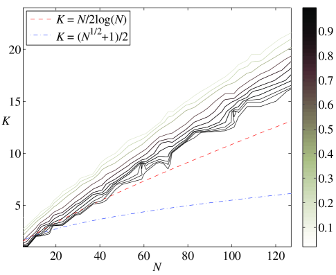
Figure 2: Numerical results from 100 independent Matlab simulations implementing BP for different $(N,K)$-pairs. The solid, gray-black lines are contours whose values represent the fraction of successful recoveries vs. the $N$-$K$ domain. The dashed, red line shows that Theorem 2 is overly pessimistic. The region below this is the zone of “perfect reconstruction.” The lower dash-dotted, blue line illustrates that Theorem 1 is too strict.

IV Radar

IV-A Classical Radar Primer

Consider the following simple (narrowband) 1-dimensional, monostatic, single-pulse, far-field radar model. Monostatic refers to the setup where the transmitter (Tx) and receiver (Rx) are collocated. The far-field assumption permits us to model the targets as point sources. Suppose a target located at range $x$ is traveling with constant velocity $v$ and has reflection coefficient $s_{xv}$. Figure 3 shows such a radar with one target. After transmitting signal $f(t)$, the receiver observes the reflected signal

$$r(t)\;=\;s_{xv}\>\!f(t-\tau_{x})\>\!\mathrm{e}^{2\pi\mathrm{i}\omega_{v}t},$$ (13)

where $\tau_{x}=2x/c$ is the round trip time of flight, $c$ is the speed of light, $\omega_{v}\approx-2\omega_{0}v/c$ is the Doppler shift, and $\omega_{0}$ is the carrier frequency. The basic idea is that the range-velocity information $(x,v)$ of the target can be inferred from the observed time delay-Doppler shift $(\tau_{x},\omega_{v})$ of $f$ in (13). Hence, a time-frequency shift operator basis is a natural representation for radar systems [23].

Figure 3: Simplified radar model. Tx transmits signal $f$, and Rx receives the reflected (or echoed) signal $r$ according to (13).

Using a matched filter at the receiver, the reflected signal $r$ is correlated with a time-frequency shifted version of the transmitted signal $f$ via the cross-ambiguity function (1)

$$|\mathcal{A}_{rf}(\tau,\omega)| = \Big{|}\!\int_{\mathbb{R}}\!r(t)\>\!\overline{f(t-\tau)}\>\!\mathrm{e}^{-2\pi\mathrm{i}\omega t}dt\>\!\Big{|}$$ (14)

$$= |\>\!s_{xv}\>\!V_{f}\!f(\tau-\tau_{x},\omega-\omega_{v})|$$

$$= |\>\!s_{xv}\>\!\mathcal{A}_{f}(\tau-\tau_{x},\omega-\omega_{v})|.$$

From this we see that the time-frequency plane consists of the ambiguity surface of $f$ centered at the target’s “location” $(\tau_{x},\omega_{v})$ and scaled by its reflection coefficient $|s_{xv}|$. Extending (14) to include multiple targets is straightforward. Figure 4 illustrates an example of the time-frequency plane with five targets; two of these have overlapping uncertainty regions. The uncertainty region is a rough indication of the essential support of $\mathcal{A}_{f}$ in (3). Targets which are too close will have overlapping ambiguity functions. This may blur the exact location of a target, or make uncertain how many targets are located in a given region in the time-frequency plane. Thus, the range-velocity resolution between targets of classical radar is limited by the radar uncertainty principle.

Figure 4: The time-frequency plane discretized into an $N\times N$ grid. Shown are five targets with their associated uncertainty regions. Classical radar detection techniques may fail to resolve the two targets whose regions are intersecting. In contrast, compressed sensing radar will be able to distinguish them as long as the total number of targets is much less then $N^{2}$.

IV-B Compressed Sensing Radar

We now propose our stylized compressed sensing radar which under appropriate conditions can “beat” the classical radar uncertainty principle! Consider $K$ targets with unknown range-velocities and corresponding reflection coefficients. Next, discretize the time-frequency plane into an $N\times N$ grid as depicted in Figure 4. Recognizing that each point on the grid represents a unique time-frequency shift $\boldsymbol{H}_{i}$ (10) (with a corresponding reflection coefficient $s_{i}$), it is easy to see that every possible target scene can be represented by some matrix $\boldsymbol{H}$ (6). If the number of targets $K\ll N^{2}$, then the time-frequency grid will be sparsely populated. By “vectorizing” the grid, we can represent it as an $N^{2}\!\times 1$ sparse vector $\boldsymbol{s}$.

Assume that the Alltop sequence $\boldsymbol{f}_{\!\mbox{\footnotesize{A}}}$ is sent by the transmitter. The received signal now is of the form in (7). If the number of targets obey the sparsity constraints in Theorems 1-3 then we will be able to reconstruct the original target scene using compressed sensing techniques. Moreover, the resolution of the recovered target scene is limited by how the time-frequency plane is discretized as dictated by the $N^{2}$ unique time-frequency shifts. That is, multiple targets located at adjacent grid points can be resolved due to the nature of compressed sensing reconstruction. The effect of discretization on the resolution is discussed in more detail in the next section.

In reality, we are not actually “beating” the classical uncertainty principle as claimed above. Rather, we are just transferring to a different mathematical perspective. The new compressed sensing uncertainty principle is dictated by the sparsity constraints of Theorems 1-3.

It is interesting to note that Alltop specifically mentions the applicability of his sequence to spread-spectrum radar. The cubic phase in (12) is known in classical radar as a discrete quadratic chirp, which is similar to what bats use to “image” their environment (although bats use a continuous sonar chirp). The use of a chirp is an effective way to transmit a wide-bandwidth signal over a relatively short time duration. However, here in compressed sensing radar we make use of the incoherence property of the Alltop sequence, which is due to specific properties of prime numbers. Recall the three key points of this novel approach: (1) the transmitted signal must be incoherent, (2) there is no matched filter, (3) instead, compressed sensing techniques are used to recover the sparse target scene.

IV-C Comparison of Resolution Limits

In this section we analyze the resolution limit for compressed sensing radar and compare it to the resolution limit dictated by the radar uncertainty principle.

Assume that the transmitted signal is bandlimited to $[-\frac{1}{2}B_{1},\frac{1}{2}B_{1}]$. Actually, the received signal will have a somewhat larger bandwidth $B>B_{1}$ due to the Doppler effect. However, in practice this increase in bandwidth is small, so we can assume $B\approx B_{1}$. We observe the signal over a duration $T$ and for simplicity sample it at the Nyquist rate $B$. That means we gather $N=BT$ many samples during the observation interval. It is well-known that observing a signal over a duration period $T$ gives rise to a maximum frequency resolution of $1/T$. The time resolution is equal to the Nyquist sampling rate, i.e., $1/B$. The step-size for the discretization of the time-frequency plane is therefore limited to $1/T$ and $1/B$, respectively.

If $N\geq 5$ is prime then we can use the Alltop sequence as described in the previous section and recover multiple targets with a resolution of $1/N$. Otherwise, there exist other “incoherent” sequences which can provide similar results to Theorems 1-3; and therefore, can also achieve a resolution of $1/N$. Thus for fixed $T$ and fixed $B$, the smallest rectangle in the time-frequency plane which can be resolved with compressed sensing radar has size $1/T\times 1/B=1/N$.

Now consider the Heisenberg uncertainty box associated with the radar uncertainty principle. When $\varepsilon=0$ in (4) this box must have an area of at least unity. This lower bound determines the resolution limit of classical radar. Juxtapose this with the resolution limit of compressed sensing: we can easily make this box smaller by increasing the observation period $T$ and/or the bandwidth $B$. Therefore, in theory, compressed sensing radar can achieve better resolution than conventional radar.

Can we achieve an even better resolution than $1/N$ for fixed duration $T$ and fixed bandwidth $B$ with compressed sensing radar? Not with the existing theory and the existing algorithms. To achieve better resolution one might be tempted to increase the sampling rate. However, oversampling introduces correlations between the samples, therefore it would not improve the incoherence of the columns of $\boldsymbol{\Phi}$ (in practice though we always oversample signals, but for different reasons).

The lower limit of $1/(TB)$ appears in other areas of classical radar as well, usually in the context of “thumbtack” functions. A function is “thumbtack-like” if all of its values are close to zero except for a unique large spike. These waveforms are also sometimes referred to as “low-correlation” sequences. Due to Properties 1 and 2 of the Alltop sequence in Section III-D we see that its ambiguity surface actually has this thumbtack feature too. Other thumbtack-like ambiguity surfaces include those associated with the waveforms which generate the equiangular line sets found in [24]. The crucial difference here is that, in general, the lower resolution limit of $1/(TB)$ can only be achieved in classical radar if there is just one target. As soon as several targets are clustered together then interference from the non-zero portions of the ambiguity function causes false positives. This dictates the resolution limit, i.e., how close targets can be and still be able to reliably distinguish them. The next section show computer simulations which demonstrate this.

IV-D Compressed Sensing and Classical Radar Simulations

Figures 5 and 6 show the result of Matlab radar simulations. For purposes of normalization the grid spacing in these figures is ${1}/{\sqrt{N}}$. Hence, the numbers shown on the axes represent multiples of ${1}/{\sqrt{N}}$. A random time-frequency scene with $K=8$ targets and $N=47$ is presented in Figure 5. The compressed sensing radar simulation used the Alltop sequence to identify the targets. In the noise-free case of Figure 5 it is clear that compressed sensing was able to perfectly reconstruct the target scene ($\|\boldsymbol{s}-\boldsymbol{s^{\bigstar}}\|_{2}\sim 10^{-8}$). Moreover, it is obvious that targets located at adjacent grid points can be resolved, confirming the discussion of the last section.

Figure 5 shows how compressed sensing starts to suffer in the presence of additive white Gaussian noise (AWGN). Here the signal-to-noise ratio (SNR) is 15 dB. Some faint false positives have appeared, yet the target scene has still been identified. The performance with 5 dB SNR is shown in Figure 5. One target was lost, many false positives have appeared, and the magnitudes of the targets have been significantly reduced. Clearly, these are all undesirable effects. It remains an open problem in the compressed sensing community how to deal with such noisy situations.

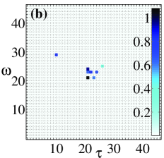
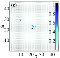
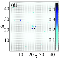
Figure 5: Radar simulation with $K=8$ targets on a $47\times 47$ time-frequency grid. (a) Original target scene. Compressed sensing reconstruction of original target scene with SNR: (b) $\infty$ dB, (c) 15 dB, (d) 5 dB. Notice in (b) that compressed sensing perfectly recovers (a) in the case of no noise.

As a comparison to compressed sensing Figure 6 presents classical radar reconstruction (which uses a matched filter as described in Section IV-A) with two different transmitted pulses. The ambiguity surfaces associated with these two waveforms demonstrate, in some sense, two extremes of traditional radar performance. In the first case, the ambiguity surface is a relatively wide Gaussian pulse, whereas in the second case the ambiguity surface is a highly concentrated “thumbtack” function. We stress that these are not necessarily the final results of traditional target reconstruction, and are included only for rough comparison. In practice, radar engineers use extremely advanced techniques to determine target range and velocity.

Figures 6, 6, and 6 show the original target scene of Figure 5 reconstructed using a Gaussian pulse. The (self) ambiguity function associated with a Gaussian pulse is a two-dimensional (2D) Gaussian pulse as a result of the STFT in (2). Therefore, according to (14) we see that the radar scenes in these figures consist of a 2D Gaussian pulse centered at each target in the time-frequency plane. In each of these it is clear that the targets in the center are contained within the Heisenberg boxes of its neighbors. Depending on the sophistication of subsequent algorithms some of the targets may be unresolvable. It is also apparent that Figures 6 and 6 suffer from added noise, and this compounds the problem of accurate resolution [4].

As a consequence of the grid spacing, the Heisenberg box associated with the Gaussian pulse’s ambiguity surface has been normalized to a square of unit area. This roughly corresponds to the support size of $U$ in (4), and is empirically verified in Figure 6 where we see that the diameter of the uncertainty region around the isolated target at $(\tau,\omega)=(10,29)$ spans approximately seven grid points. Since the grid spacing is ${1}/{\sqrt{N}}$ we confirm that the base and height of the Heisenberg box are each approximately ${7}/{\sqrt{47}}\approx 1$.

Returning to the discussion of the previous section, it is clear that the noise-free cases shown in Figures 5 and 6 experimentally confirm that compressed sensing radar can achieve much higher resolution than traditional techniques. To make the comparison fair, we are using the same number of observations in the recovery for both compressed sensing and classical radar. In this sense, it becomes apparent that we are leveraging the power of compressed sensing theory in a different way than explained in Section II. The typical compressed sensing application makes far fewer observations than necessary and still obtains perfect reconstruction of the data. However, in this model of compressed sensing radar we implicitly assume Nyquist sampling of the baseband signal. Therefore, with this setup, the benefit of employing compressed sensing recovery manifests itself as a dramatic increase in resolution.

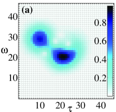
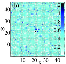
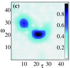
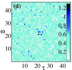
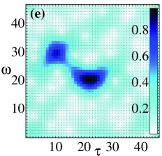
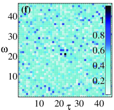
Figure 6: Traditional radar reconstruction of Fig. 5’s original target scene. With no noise: (a) Gaussian pulse, (b) Alltop sequence. With SNR = 15 dB: (c) Gaussian pulse, (d) Alltop sequence. With SNR = 5 dB: (e) Gaussian pulse, (f) Alltop sequence.

In contrast with a Gaussian pulse we now examine a waveform whose associated ambiguity surface is thumbtack-like. Figures 6, 6, and 6 depict the original target scene traditionally reconstructed using the Alltop sequence. Take note of the distinction with compressed sensing radar presented in Section IV-B which also uses this function. Here, the classical approach transmits the Alltop sequence, and then uses a matched filter to correlate the received signal with a time-frequency shifted Alltop sequence as in (14). The radar scene will now consist of a thumbtack function centered at each target. In theory, this radar would provide target resolution similar to our compressed sensing version (i.e., the target is represented as a point source in time-frequency plane rather than a “spread out” uncertainty region).

However, the situation is not so simple. The non-zero portions of the ambiguity function can accumulate to create undesirable effects. This is shown in Figure 6 where it is apparent, even in the ideal case of no added noise, that there is a great deal of interference. Moreover, this type of “noise” is deterministic and cannot be remedied by averaging over multiple observations. Notice that the interference seems to be distributed over a wide range of amplitudes. In fact, referring to the original target scene in Figure 5, it appears that some of the weaker targets (i.e., the ones with the smallest reflection coefficient in magnitude) have been buried in this noise. Even if a reasonable threshold could be determined, perhaps only a few of the strongest targets would be detected and many false positives would remain. This is a substantial problem since the dynamic range of the targets can be quite large.

We present these results to emphasize that naive application of traditional radar techniques with the Alltop sequence will fail if the radar scene contains more than just a few strong targets. The outcome will be similar if other low-correlation sequences are used.

Regardless of whether a transmitted waveform has an ambiguity surface which is spread or narrow, interference from adjacent targets will necessarily occur in classical radar, and this will result in undesirable effects. In contrast, compressed sensing radar does not experience this interference since it completely dispenses with the need for a matched filter. Therefore, there are no issues with the ambiguity function of the transmitted signal.

V Other Applications

Narrowband radar is by no means the only application to which the techniques presented here can be used. Wideband radar systems admit a received signal which is of the form

$$|r(t)|\;\sim\;\Big{|}f\Big{(}\frac{t-a\>\!\tau_{x}}{a}\Big{)}\Big{|},\qquad a=1-2v/c.$$

This shift-scaled signal is well-represented by a wavelet basis, and it seems feasible to replace the time-frequency dictionary by a properly chosen time-scale dictionary. In a different direction, the methods introduced in this paper can also be extended to multiple-input multiple-output (MIMO) radar systems.

Our approach can also be applied, with suitable modifications, to other applications that involve the identification of a linear (time-varying) system. For instance, a challenging task in underwater acoustic communication is the estimation of the acoustic propagation channel. Unlike mobile radio channels, underwater acoustic channels often exhibit large delay spreads with substantial Doppler shifts. Of course, the location of the scatterers and the amount of Doppler shift are a priori not known. However, it is known that underwater communication channels do have a sparse representation in the time-frequency domain, e.g., see [14]. Thus, there is a good chance that our approach via compressed sensing can lead to a channel estimation method that provides higher resolution than conventional methods. We point out that in order to turn compressed sensing-based underwater acoustic channel estimation into a reliable method, one needs to carefully incorporate various other properties of underwater environments, e.g., whether we are dealing with a deep sea environment or a shallow water environment.

Another application where the proposed compressed sensing approach seems useful arises in high-resolution radar imaging. For instance, when we consider the imaging of (moving) point targets, one would need to combine our time-frequency based approach with the Born approximation of Helmholtz’s equation. This approach is a topic of our current research.

Other applications arise in blind source separation [15], sonar, as well as underwater acoustic imaging based on matched field processing.

VI Discussion

We have provided a sketch for a high-resolution radar system based on compressed sensing. Assuming that the number of targets obey the sparsity constraint in Theorem 2, the Alltop sequence can perfectly identify the radar scene with high probability using compressed sensing techniques. Numerical simulations confirm that this sparsity constraint is too strict and can be relaxed to $K\leq N/(2\log{N})$, although this has yet to be proven mathematically.

It must be emphasized that our model presents radar in a rather simplified manner. In reality, radar engineers employ highly sophisticated methods to identify targets. For example, rather than a single pulse, a signal with multiple pulses is often used and information is averaged over several observations. We also did not address how to discretize the analog signals used in both compressed sensing and classical radar. A more detailed study covering these issues is the topic of another paper.

Related to the discretization issue is the fact that compressed sensing radar does not use a matched filter at the receiver. This will directly impact A/D conversion, and has the potential to reduce the overall data rate and to simplify hardware design. These matters are discussed in [1], although it does not consider the case of moving targets. In our study the major benefit of relinquishing the matched filter is to avoid the target uncertainty and interference resulting from the ambiguity function.

Since many of the implementation details of our compressed sensing radar have yet to be determined, and since classical radar can also be implemented in many ways we were only able to make a rough comparison between their respective resolutions. Regardless, the radar uncertainty principle lies at the core of traditional approaches and limits their performance. We contend that compressed sensing provides the potential to achieve higher resolution between targets. The radar simulations presented confirm this claim.

It must be stressed again that the success of this stylized compressed sensing radar relied on the incoherence of the dictionary $\boldsymbol{\Phi}_{\!\mbox{\footnotesize{A}}}$ resulting from the Alltop sequence. There exist other probing functions with similar incoherence properties. Numerical simulations with $\boldsymbol{f}$ as a random Gaussian signal, as well as a constant-envelope random-phase signal indicate similar behavior to what we have reported for the Alltop sequence. At the time of writing this paper we became aware of a similar study [25] where the properties of these functions are analyzed in the context of abstract system identification using compressed sensing.

There is also the possibility of combining classical radar techniques with $\ell_{1}$ recovery. Initial tests show that while we get good reconstruction, the results are not guaranteed, even in the case of no noise. Figure 7 shows a striking example. In this noise-free scenario, a Gaussian pulse has been transmitted and reconstruction is done using $\ell_{1}$ minimization. Figure 7 shows an original radar scene with $K=3$ targets. It is clear from Figure 7 that none of the targets have been correctly recovered. In contrast, Theorem 1 proves that we are guaranteed to perfectly recover both of these target scenes when transmitting the Alltop sequence. (Note, in order to employ Theorem 1, we need to satisfy $K<\frac{1}{2}(\sqrt{N}+1)$. With $N=47$ we can only use $K=3$ targets since $3<\frac{1}{2}(\sqrt{47}+1)\approx 3.93$.)

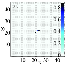
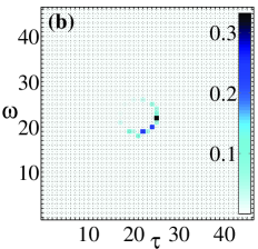
Figure 7: Radar simulation with $K=3$ targets on a $47\times 47$ time-frequency grid. (a) Original target scene. (b) Traditional Gaussian pulse and reconstruction using $\ell_{1}$ minimization (no noise). It is clear that conventional radar with $\ell_{1}$ minimization completely fails. However, Theorem 1 guarantees perfect recovery in this case.

Appendix A Proof of the Theorems

For notational simplicity denote the coherence of dictionary $\boldsymbol{\Phi}$ as $\mu$. We need the following theorems which deal with incoherent dictionaries such as $\boldsymbol{\Phi}_{\!\mbox{\footnotesize{A}}}\in\mathbb{C}^{N\times N^{2}}$. Recall for $\boldsymbol{\Phi}_{\!\mbox{\footnotesize{A}}}$ that $\mu={1}/{\sqrt{N}}$ with prime $N\geq 5$.

Proposition 1 ([26], Theorem B).

Let $\boldsymbol{X}$ be a random $K$-column subdictionary of $\boldsymbol{\Phi}$ (i.e, every $K$-column subset of $\boldsymbol{\Phi}$ has an equal probability of being chosen). The condition $\sqrt{\mu^{2}K\log{K}\cdot\vartheta}+\frac{K}{N^{2}}\|\boldsymbol{\Phi}\|^{2}\leq c\delta$ with $\vartheta\geq 1$ implies that ${\mathbb{P}}{\{\|\boldsymbol{X^{*}X}-\boldsymbol{I}\|\geq\delta\}}\leq K^{-\vartheta}$ where $c$ is an absolute constant.

Proposition 2 ([26], Theorem 14).

Suppose random $\boldsymbol{s}\in\mathbb{C}^{N^{2}}$ has support $T$, sparseness $K=|T|$, and nonzero coefficients whose phases are uniformly distributed on the interval $[0,2\pi)$. Set $\boldsymbol{y}\;\!=\;\!\boldsymbol{\Phi}\boldsymbol{s}$, and let $\boldsymbol{\Phi}_{T}$ be the submatrix consisting of the columns $\boldsymbol{\varphi}_{j}$ of $\boldsymbol{\Phi}$ for $j\in T$. Suppose $8\mu^{2}K\leq 1/\log{(N^{2}\!/\zeta)}$ and that the least singular value $\sigma_{\min}(\boldsymbol{\Phi}_{T})\geq 1/\sqrt{2}$. Then $\boldsymbol{s}$ is the unique solution to BP except with probability $2\zeta$.

Proposition 3 ([27], Theorem 3).

Suppose a noisy signal $\boldsymbol{y}=\boldsymbol{\Phi}\boldsymbol{s}+\boldsymbol{e}$ is constructed as a sparse combination of the columns of dictionary $\boldsymbol{\Phi}\in\mathbb{C}^{N\times N^{2}}$ with coherence $\mu$. Assume the sparsity of $\boldsymbol{s}$ obeys $K<(1+\mu)/(2\mu+4\varepsilon\sqrt{N}/T)$, and the entries of the noise are bounded $|e_{n}|\leq\varepsilon$. Then the solution $\boldsymbol{s^{\bigstar}}$ to BP exhibits stability $\|\boldsymbol{s}-\boldsymbol{s^{\bigstar}}\|_{1}\leq T$.

A-A Theorem 1

Proof:

Theorem B in [7] (which incorporates results from [27], [28], and [29]) concludes for general dictionary $\boldsymbol{\Phi}$ that every $K$-sparse signal $\boldsymbol{s}$ with $K<\frac{1}{2}(\mu^{-1}+1)$ is the unique sparsest representation, and is guaranteed to be recovered by both BP and OMP when observing $\boldsymbol{y}=\boldsymbol{\Phi}\boldsymbol{s}$. Set $\boldsymbol{\Phi}=\boldsymbol{\Phi}_{\!\mbox{\footnotesize{A}}}$ and assume the hypothesis of Theorem 1. Equation (7) provides $\boldsymbol{y}=\boldsymbol{H}\boldsymbol{f}_{\!\mbox{\footnotesize{A}}}=\boldsymbol{\Phi}_{\!\mbox{\footnotesize{A}}}\boldsymbol{s}$. The result follows by substituting ${\mu=1/{\sqrt{N}}}$. ∎

A-B Theorem 2

Proof:

Set $\boldsymbol{\Phi}=\boldsymbol{\Phi}_{\!\mbox{\footnotesize{A}}}$. Let $\mathscr{A}$ denote the event that $\|\boldsymbol{X^{*}X}-\boldsymbol{I}\|<\frac{1}{2}$, and let $\mathscr{B}$ represent the event that BP recovers random $\boldsymbol{s}$ from the observation $\boldsymbol{y}=\boldsymbol{H}\boldsymbol{f}_{\!\mbox{\footnotesize{A}}}=\boldsymbol{\Phi}_{\!\mbox{\footnotesize{A}}}\boldsymbol{s}$. Proposition 1 concerns ${\mathbb{P}}{(\mathscr{A}^{\complement})}$ where $\mathscr{A}^{\complement}$ is the complement of set $\mathscr{A}$, and Proposition 2 addresses ${\mathbb{P}}{(\mathscr{B}|\mathscr{A})}$. To apply these propositions we need their conditions to be satisfied simultaneously. Since $\boldsymbol{\Phi}_{\!\mbox{\footnotesize{A}}}$ is a unit-norm tight frame we know that $\|\boldsymbol{\Phi}_{\!\mbox{\footnotesize{A}}}\|^{2}=N$. With $\mu={1}/{\sqrt{N}}$ and taking $\delta=\frac{1}{2}$ the condition of Proposition 1 is

$$\sqrt{\frac{K}{N}\log{K}\cdot\vartheta}\;+\;\frac{K}{N}\;\leq\;\frac{c}{2}.$$ (15)

Fix $\zeta=\varepsilon^{2}$ for some sufficiently small desired probability of error in Proposition 2. The sparsity condition can now be rewritten as $K\leq N/(16\log{(N/\varepsilon)})$. Substituting this into (15) the LHS is less than

$$\!\!\!\!\!\!\!\!\!\!\!\!\!\!\!\!\!\!\!\!\!\!\!\!\!\!\!\!\!\!\sqrt{\frac{\vartheta}{16\log{(N/\varepsilon)}}\log\Big{(}\frac{N}{16\log{(N/\varepsilon)}}\Big{)}}\;+\;\frac{1}{16\log{(N/\varepsilon)}}$$ (16)

$$< \sqrt{\frac{\vartheta}{16\log{(N/\varepsilon)}}\log{{N}}}\;+\;\sqrt{\frac{1}{16\log{(N/\varepsilon)}}}$$

$$< \frac{1}{2}\sqrt{\frac{\vartheta\;\!{\log{{N}}}}{\log{(N/\varepsilon)}}}\qquad\mbox{(since $\vartheta,\log{N}\geq 1$)}.$$

Choose $\vartheta\geq 1$ such that $\sqrt{{\vartheta\;\!{\log{{N}}}}/{\log{(N/\varepsilon)}}}\leq c$ is satisfied. Assume the other conditions of Proposition 2 (observe that event $\mathscr{A}$ implies $\sigma_{\min}(\boldsymbol{\Phi}_{T})\geq 1/\sqrt{2}$), and let $\boldsymbol{X}=\boldsymbol{\Phi}_{T}$ in Proposition 1. Then

$${\mathbb{P}}{(\mathscr{B})} \geq {\mathbb{P}}{(\mathscr{B}|\mathscr{A})}\;\!{\mathbb{P}}{(\mathscr{A})}$$ (17)

$$\geq (1-2\varepsilon^{2})(1-K^{-\vartheta})$$

$$> 1-2\varepsilon^{2}-K^{-\vartheta}$$

as desired.∎

A-C Theorem 3

Proof:

As in the proof of Theorem 1, this follows immediately mutatis mutandis. ∎

References

- [1] R. Baraniuk and P. Steeghs, “Compressive radar imaging,” Proc. 2007 IEEE Radar Conf., pp. 128–133, Apr. 2007.
- [2] R. E. Blahut, “Theory of remote surveillance algorithms,” in Radar and Sonar, Part I, ser. IMA Volumes in Mathematics and its Aplications, R. E. Blahut, W. Miller Jr., and C. H. Wilcox, Eds. NY: Springer-Verlag, 1991, vol. 32, pp. 1–65.
- [3] K. Gröchenig, “Uncertainty principles for time-frequency representations,” in Advances in Gabor Analysis, ser. Applied and Numerical Harmonic Analysis, H. G. Feichtinger and T. Strohmer, Eds. Boston: Birkhäuser, 2003, pp. 11–30.
- [4] A. W. Rihaczek, High-Resolution Radar. Boston: Artech House, 1996, (originally published: McGraw-Hill, NY, 1969).
- [5] D. L. Donoho, “Compressed sensing,” IEEE Trans. Inf. Theory, vol. 52, no. 4, pp. 1289–1306, 2006.
- [6] E. J. Candès, J. Romberg, and T. Tao, “Robust uncertaitny principles: Exact signal reconstruction from highly incomplete frequency information,” IEEE Trans. Inf. Theory, vol. 52, no. 2, pp. 489–509, Feb. 2006.
- [7] J. A. Tropp, “Greed is good: Algorithmic results for sparse approximation,” IEEE Trans. Inf. Theory, vol. 50, no. 10, pp. 2231–2242, Oct. 2004.
- [8] D. Needell and R. Vershynin, “Uniform uncertainty principle and signal recovery via regularized orthogonal matching pursuit,” July 2007, preprint.
- [9] R. A. Rankin, “The closest packing of spherical caps in dimensions,” Proc. Glasgow Math. Assoc., vol. 2, pp. 139–144, 1955.
- [10] L. R. Welch, “Lower bounds on the maximum cross-correlation of signals,” IEEE Trans. Inf. Theory, vol. 20, no. 3, pp. 397–399, 1974.
- [11] P. Delsarte, J. M. Goethals, and J. J. Seidel, “Bounds for systems of lines and Jacobi poynomials,” Philips Res. Repts, vol. 30, no. 3, pp. –, 1975, issue in honour of C.J. Bouwkamp.
- [12] K. Gröchenig, Foundations of time-frequency analysis. Boston: Birkhäuser, 2001.
- [13] P. A. Bello, “Characterization of randomly time-variant linear channels,” IEEE Trans. on Comm., vol. 11, no. 4, pp. 360–393, Dec. 1963.
- [14] W. Li and J. C. Preisig, “Estimation and equalization of rapidly varying sparse acoustic communication channels,” Proc. IEEE OCEANS 2006, pp. 1–6, Sept. 2006.
- [15] Z. Shan, J. Swary, and S. Aviyente, “Underdetermined source separation in the time-frequency domain,” Proc. IEEE ICASSP 2007, pp. 945–948, April 2007.
- [16] W. O. Alltop, “Complex sequences with low periodic correlations,” IEEE Trans. Inf. Theory, vol. 26, no. 3, pp. 350–354, May 1980.
- [17] M. Planat, H. C. Rosu, and S. Perrine, “A survey of finite algebraic geometrical structures underlying mutually unbiased quantum measurements,” Foundations of Physics, vol. 36, no. 11, pp. 1662–1680, Nov. 2006.
- [18] T. Strohmer and R. Heath Jr., “Grassmannian frames with applications to coding and communications,” Appl. Comp. Harm. Anal., vol. 14, no. 3, pp. 257–275, 2003.
- [19] D. M. Appleby, “Symmetric informationally complete–positive operator valued measures and the extended Clifford group,” Journal Math. Phys., vol. 46, 2005, 052107.
- [20] D. Tse and P. Viswanath, Fundamentals of Wireless Communication. Cambridge: Cambridge University Press, 2005.
- [21] M. Grant, S. Boyd, and Y. Ye, “cvx: Matlab software for disciplined convex programming.” [Online]. Available: http://www.stanford.edu/boyd/cvx/
- [22] MOSEK Optimization Software, http://mosek.com/.
- [23] L. Auslander and R. Tolimieri, “Radar ambiguity functions and group theory,” SIAM Journal on Mathematical Analysis, vol. 16, no. 3, pp. 577–601, 1985.
- [24] S. D. Howard, A. R. Calderbank, and W. Moran, “The finite Heisenberg-Weyl groups in radar and communications,” EURASIP Journal on Applied Signal Processing, vol. 2006, pp. 1–12, article ID 85685.
- [25] G. E. Pfander, H. Rauhut, and J. Tanner, “Identification of matrices having a sparse representation,” June 2007, preprint.
- [26] J. A. Tropp, “On the conditioning of random subdictionaries,” Aug. 2007, preprint.
- [27] D. L. Donoho and M. Elad, “On the stability of the basis pursuit in the presence of noise,” EURASIP Signal Processing Journal, vol. 86, no. 3, pp. 511–532, Mar. 2006.
- [28] M. Elad and A. Bruckstein, “A generalized uncertainty principle and sparse representation in pairs of bases,” IEEE Trans. Inf. Theory, vol. 48, no. 9, pp. 2558–2567, Sept. 2002.
- [29] R. Gribonval and M. Nielsen, “Sparse representations in union of bases,” IEEE Trans. Inf. Theory, vol. 49, no. 12, pp. 3320–3325, Dec. 2003.