The Anatomy of Mitos Web Search Engine

Abstract

Engineering a Web search engine offering effective and efficient information retrieval is a challenging task. This document presents our experiences from designing and developing a Web search engine offering a wide spectrum of functionalities and we report some interesting experimental results. A rather peculiar design choice of the engine is that its index is based on a DBMS, while some of the distinctive functionalities that are offered include advanced Greek language stemming, real time result clustering, and advanced link analysis techniques (also for spam page detection).

1 Introduction

Engineering a Web search engine offering effective and efficient information retrieval is a challenging task. The objective of this document is to present our experiences from designing and developing Mitos (previously named groogle), a currently emerged search engine that offers a wide spectrum of functionalities. Distinctive functionalities include: (a) an advanced stemmer for the Greek language, (b) real time result clustering, (c) advanced link analysis techniques (also for spam detection).

Apart from describing the overall architecture and component specifications, we report some interesting experimental results regarding all associated tasks (i.e. crawling, stemming, stopwords elimination, indexing, query evaluation, clustering). One crucial design choice of Mitos is that its index is based on a DBMS. This choice has some benefits and some drawbacks. An advantage is that we can exploit all amenities offered by a DBMS. To the problem at hand, some benefits include: (a) efficient index update (e.g. efficient deletion of those index entries that concern web pages that no longer exist, or addition of newly crawled or submitted web pages), and (b) straightforward extension of the index schema with additional columns and relations (e.g. for widening the spectrum of functionalities offered). The drawbacks include higher storage space requirements and poorer performance in certain tasks. To clarify this aspect, we compare our engine with other well-known inverted file-based IR systems (like Terrier) and discuss the results of this comparison.

The rest of this paper is organized as follows: Section 2 describes the overall architecture of the engine. Section 3 describes briefly each component. Section 4 reports experimental results, and finally, Section 5 concludes the paper and identifies issues for further work and research.

2 Architectural Overview

This section gives a high level overview of the architecture and the functioning of the system. Most components of Mitos  are implemented in Java 5 to preserve platform-independent deployment. The current installation of Mitos runs on a single machine (Pentium IV 3.2GHz, 2GB RAM, Debian) and is accessible through http://groogle.csd.uoc.gr:8080/mitos/.

Two are the basic processes: the indexing process that is performed offline and the searching process that is performed every time a user is searching for something based on a query. Figure 1 illustrates the component diagram and outlines the indexing and retrieval process.

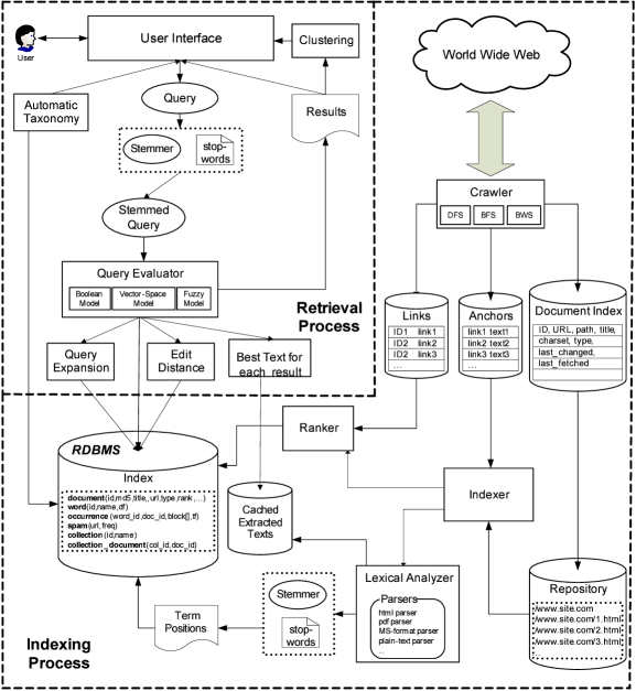
Figure 1: The Component Model of Mitos

At the indexing phase, the crawler is responsible for recursively fetching Web pages given a starting list of URLs to visit. The fetched pages are stored in a local repository for further processing. Each downloaded page is assigned a unique ID number and that number is used for referring to that page (e.g. in Links). The crawler also builds a Document Index that maps the ID of each page with its url and other useful properties (like path, title, last changed/fetched, etc). In addition, it stores the hyperlinks (including the anchor texts) in the file Links. This file is useful for various link analysis-based ranking techniques (like PageRank). The contents of the pages in the repository are indexed by the Indexer. At first, the Lexical Analyzer identifies tokens, removes stopwords and applies stemming algorithms. Then documents are seen as vectors of terms and the Index is created using a relational DBMS. For each document, its word occurrences, their weights and the PageRank of the document is stored. The exact positions of each word occurrence in a document can be optionally stored. In addition, the full text of documents is extracted and stored locally (in order to enable the derivation of document surrogates while presenting the results of retrieval) The exact process is described later in Section 3.5.

The retrieval process starts after the submission of a user query. Several retrieval models are supported (Section 3.7). If a query term does not exist in the lexicon, the system suggests replacing that term with terms that exist and whose Edit Distance (from the submitted term) is less than a threshold. Moreover, for each query the system suggests a list of terms which could be used to expand (refine) the submitted query (these terms are derived by analyzing the top-ranked documents). Regarding the presentation of the search results, each document is presented by a surrogate that includes a short indicative excerpt (containing as much of the query terms as possible). In addition, search results are optionally clustered into different groups, so that each group share some common trait. Various clustering algorithms are supported (Section 3.9).

Mitos offers a number of auxiliary modules including a module for automatically constructing taxonomies (Section 3.10) and a module for aiding the detection of spam pages in particular it identifies the subset of the fetched pages that are worth inspecting by a human (the pages that are manually marked as spam, are then taken into account by the link analysis-based ranking techniques).

3 Components Description

This section describes each component in more detail. Table 1 shows some notations that will be used in the sequel.

Table 1: Notations

Symbol	Meaning
$N$	Number of documents indexed at the repository
$E$	Number of web links at the repository
$K$	Edit distance tolerance
$L$	Number of top pages used in query expansion and clustering,
	levels of automatic taxonomy
$M$	Levels with highest frequencies in automatic taxonomy
$S$	Number of query expansion suggested terms
$V$	Vocabulary
$q$	query
$|q|$	number of words in the query
$|ans(q)|$	number of documents with not empty degree of relevance with $q$

Regarding experiments, we crawled all documents of our university department (http://www.csd.uoc.gr) and FORTH-ICS (http://www.ics.forth.gr) web sites. The whole collection is approximately 2.8 GB. About 32% of the files use a Greek character encoding.

3.1 Crawler

The crawler roams the web, identifies all the hyperlinks in each page and adds them to a list of URLs to visit. URLs are then recursively visited according to a set of policies. Currently, three traversal policies are supported: Breadth-first (BFS), Depth-first (DFS) and Depth-within-site (DWS). Crawler can be configured to download only files of a specific type (e.g. html, pdf, rdf) as well as to ignore others based on extension (e.g. *.tmp). The identification of files is based on extension and on content for dynamic web pages. Furthermore it is compatible with the Robots Exclusion Protocol to ignore specified files or directories. The downloaded documents are stored in the local file system. Each web site occupies a different directory that has the name of its domain (e.g. http://www.cnn.com will be stored under the directory ./www.cnn.com) and its documents are stored locally under the same absolute paths. A Document Index, created also by the crawler, keeps information about each document. These include the md5 of the document, its canonicalized URL, the absolute path in the disk, its title, its type (e.g. html, pdf, etc.) and the dates that was last modified and last fetched. Furthermore, the out-links of each downloaded web page are stored. The md5 of the document is computed based on its URL to eliminate the possibility that two documents will have the same hash. We have not observed any collision so far. The hash is used as a unique identifier (ID) for the document. The Document Index is used by the Indexer to analyze all downloaded documents and build the index. To overcome the time spent due to I/O latencies, the crawler uses multiple threads. Table 2 shows the time needed to download 100.000 documents from popular servers all over the world regarding the number of threads for BFS and DFS algorithms. Each thread uses one distinct site as a seed, so different threads do not overlap. The efficiency is almost the same for both algorithms. We also observe a linear speedup for the number of threads that is, however, highly dependable on the selected web servers and the link capacity.

Table 2: Times to crawl and download 100.000 pages

Number of	Traversal Algorithm
Threads	BFS	DFS
5	13552 sec	13751 sec
10	6725 sec	6687 sec
20	3562 sec	3763 sec

3.2 Lexical Analyzer

The Lexical Analyzer plays a major part in the pre-processing of the documents. It is responsible for converting a string of characters into a stream of tokens. Most IR systems use single words as terms. The Lexical Analyzer is called by the indexer for each document, with its file type and encoding as parameters. After processing the document it returns a hash map that contains all document’s words, along with their frequency and position.

The process of document analysis can be divided in the following steps:

1. Recognition of the document’s structure

2. Extraction of document’s text. The text is analyzed in tokens and the terms to be inserted in the lexicon are selected. For each token $t_{i}$ identified in the document $d_{j}$, the analyzer returns the frequency (i.e $freq_{ij}$ ), the maximum frequency (i.e $max_{k}\{freq_{kj}\;|\;t_{k}\in d_{j}\})$) of terms in the document and the positions of $t_{i}$ in $d_{j}$. Then, the frequencies are normalized by the frequency of the term that appears mostly in the document.

3. Insertion of stemmed terms into the hash map

The selection of the terms to be used as index terms determines the quality of the lexicon. Words that are considered non-informative, like function words (the, in, of, a) also called stop-words are often ignored. There is a list of stop-words which consists of 400 words (320 english and 80 greek words). The main benefit of stop-words removal is that it reduces the size of the index, however it may reduce recall (e.g. consider a user is looking for documents containing the phrase ’to be or not to be’). For this reason, some web search engines do not eliminate stop-words from documents. In Mitos, stop-words elimination is optional. Furthermore, there are options for the removal of numbers and terms consisted of both characters and numbers.

The lexical analyzer accepts the following file types: html (html, htm, php, jsp, asp), doc, ppt, pps, xls, rtf, txt. For the text extraction from the documents various software components were used, specifically pdfbox for pdf documents, Jakarta POI for doc, ppt, pps, xls, and RTFEditorKit for RDF documents. The analyzing time of each document type is shown in Table 3.

Table 3: Lexical Analysis Times

File Type	Average Time of 100 experiments (sec)
html	0.0361
pdf	0.3750
doc	0.0808
ppt	0.0732
pps	0.2630
xls	0.0983
rtf	0.1917
txt	0.0343

3.3 Stemmer (including a Greek one)

The main idea behind stemming is that users searching for information on retrieval will also be interested in articles that have information about retrieve, retrieved, retrieving, retriever, and so on. Several stemmers for various languages have been developed over the years, each with its own set of stemming rules. However, the usefulness of stemming for improved search quality has always been questioned in the research community, especially for English. The consensus is that, for English, stemming yields small improvements in search effectiveness; however, in cases where it causes poor retrieval, the user can be considerably annoyed [11].

Stemming is possibly more beneficial for languages with many word inflexions (like German and Greek) [12]. Currently there were only few stemmers for the Greek language [9]. The stemmer used in Mitos is based on the automated technique of affix removal - Porter’s Algorithm [13]. By studying the greek language grammar rules, a collection of common suffixes for nouns and adjectives was gathered, including comparative, participle, singular and plural forms in all genders and also verbs in different voices and tenses. This collection was expanded using 270 ”productive suffixes” for words produced by other words with the same semantics. The total number of suffixes used is 782. In the simple past and past continuous tenses the inflexion may be applied with a possible addition of an accentuated letter as a prefix, or internal change in case of compound words. Therefore a collection of adverbs and prothesses as prefixes was considered necessary to eliminate these inflections and derive the base word of the compound. Another point where the stemming could be problematic when using common methods of affix removal, are the irregularities of verbs. The restricted set of these words was used to reduce the semantically equal but lexically different roots into a unique root. Also a collection of unmodified words was gathered, since the stemming process would be useless. Finally, the inflexions of the last character of the root, provide according to ancient greek grammar rules, three different sets of characters and digraphs and a single character which will replace each of these sets.

The greek stemmer is initialized, using the files of suffixes, prefixes, irregular verbs and unmodified words to construct an equal number of Trie structures. The prefixes file contains 83 entries and as far as the irregular verbs is concerned, variations of 29 different verbs were used. Additional information is kept in the suffixes trie, reffering to the type, verbal or not, of the word that is matched. Also in the prefixes trie the initial form is kept as a replacement. The irregular verbs trie contains the stemmed variations and a predefined stem.

Table 4: Examples of Greek Stemmer

Word	Word Split	prefixes-First Stem	Increment-Alternate	Final Stem
$\pi\rho\alpha\tau\tau\omega$	$\pi\rho\alpha\tau\tau\omega$	$\pi\rho\alpha\tau\tau$	$\pi\rho\alpha\xi$	$\pi\rho\alpha\xi$
$\pi\rho\alpha\kappa\tau\iota\kappa o\varsigma$	$\pi\rho\alpha\kappa\tau\iota\kappa\varsigma$	$\pi\rho\alpha\kappa\tau$	$\pi\rho\alpha\xi$	$\pi\rho\alpha\xi$
$\pi\rho\alpha\xi\eta$	$\pi\rho\alpha\xi\eta$	$\pi\rho\alpha\xi$	$\pi\rho\alpha\xi$	$\pi\rho\alpha\xi$
$\pi\rho\alpha\gamma\mu\alpha$	$\pi\rho\alpha\gamma\mu\alpha$	$\pi\rho\alpha\gamma\mu$	$\pi\rho\alpha\xi$	$\pi\rho\alpha\xi$
$\alpha\nu\alpha\delta\iota\alpha\tau\alpha\xi\eta$	$\alpha\nu\alpha-\delta\iota\alpha-\tau\alpha\xi\eta$	$\alpha\nu\alpha-\delta\iota\alpha-\tau\alpha\xi$	$\alpha\nu\alpha-\delta\iota\alpha-\tau\alpha\xi$	$\alpha\nu\alpha\delta\iota\alpha\tau\alpha\xi$
$\alpha\nu\alpha\delta\iota\alpha\tau\alpha\sigma\sigma\omega$	$\alpha\nu\alpha-\delta\iota\alpha-\tau\alpha\sigma\sigma\omega$	$\alpha\nu\alpha-\delta\iota\alpha-\tau\alpha\sigma\sigma$	$\alpha\nu\alpha-\delta\iota\alpha-\tau\alpha\xi$	$\alpha\nu\alpha\delta\iota\alpha\tau\alpha\xi$
$\alpha\nu\alpha\delta\iota\epsilon\tau\alpha\xi\alpha$	$\alpha\nu\alpha-\delta\iota\epsilon-\tau\alpha\xi\alpha$	$\alpha\nu\alpha-\delta\iota\alpha-\tau\alpha\xi$	$\alpha\nu\alpha-\delta\iota\alpha-\tau\alpha\xi$	$\alpha\nu\alpha\delta\iota\alpha\tau\alpha\xi$
$\pi\alpha\omega$	$\pi\alpha\omega$	$\pi$	$\pi\eta\gamma$	$\pi\eta\gamma$
$\pi\eta\gamma\alpha\iota\nu\omega$	$\pi\eta\gamma\alpha\iota\nu\omega$	$\pi\eta\gamma$	$\pi\eta\gamma$	$\pi\eta\gamma$

A word to be stemmed is first checked whether it belongs to an unmodified words set. Currently, this set contains 291 words. The actual stemming procedure starts with the prefixes separation which produces alternative prefixes. Suffix removal is applied on the derived word after the replacement of all accented-characters. Since the current stem comes from a verbal suffix type, it is examined if it belongs to the irregular verbs in order to retrieve the replacement stem. In other cases an optimization is conducted. The optimization may increase the length of the root by one or two letters and may be followed by a last character replacement. Finally, existing prefix is reconcatenated to produce the final stem of the word. Examples of the process can be seen in Table 4.

3.4 Lexicon

We conducted some measurements in order to see the distribution of words in our collection and the effects of stemming and stop-words removal.

Figure 2a shows the frequencies of terms in the Index, when stemming is not enabled and stopwords have not been removed. One can observe that a few terms, including many stop-words (like the terms ’and’, ’the’, ’for’, ’with’, etc.) get upward of 4000 occurrences, whereas most terms got only a few occurrences (about 54% of the terms have got only a single occurrence). Specifically the index has 301052 terms with 4824739 occurences. Figure 3a shows the same plot, but on a log-log scale.

To investigate to what extent the plotted function approximates a power law, we rely on a commonly used method (based on the least square errors method), called Linear Regression [14], to fit a line in a set of 2-dimensional points and, thus, to investigate whether the log-log plot of the function approximates a line. The accuracy of the approximation is indicated by the correlation coefficient, the absolute value of which (hereafter called $ACC$) always lies in $[0,1]$. An $ACC$ value $1.0$ indicates perfect linear correlation, i.e., the points are exactly on a line. In this respect, we observed that the function plotted in Figure 2 approximates ($ACC=0.996$, i.e. $99.6\%$ confidence) a power law with exponent $1.29$.

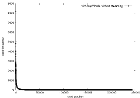
(a)

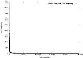
(b)

Figure 2: Linear scale plot of the words and their frequencies. In the right plot the words are stemmed and stop-words have been removed while in the left not.

Figures 2b and 3b show the term frequencies when stemming is enabled and stop-words have been removed. Now our index consists of 220518 terms (26.7% reduction caused by stemming) and 3435040 occurences (28.8% reduction caused by stopwords). That function also approximates ($ACC=0.996$) a power law but with slightly decreased exponent, i.e. $1.18$.

Although the log-log distributions of both functions follow a power law, we observe a top concavity deviation, frequently met on many datasets[6].

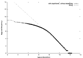
(a)

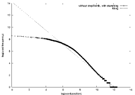
(b)

Figure 3: Log-log scale plot of the words and their frequencies. In the right plot the words are stemmed and stop-words have been removed while in the left not.

3.5 DBMS-based Indexer

The Indexer iterates through all the records of the Document Index and uses the Lexical Analyzer component to create a hash table that contains the words and their exact positions for each document in the Repository. The index is built on top of a DBMS (in particular over PostgreSQL 8.3). The database schema can be seen in Table 5.

The use of a relational DBMS is motivated by the following facts:

• it allows for incremental indexing of document collections. To the best of our knowledge, no other open-source IR system allows incremental indexing, i.e., one should always create the index from scratch. Furthermore, the ”deletion” of documents from the index (e.g. when a Web page disappears or when it is classified as spam) is efficient, while this operation is very expensive in inverted files. Savings in time and computational resources are straightforward. Moreover, this functionality is especially useful, for the IR research community, which frequently faces the need to conduct experiments on top of an IR system.

• makes our index to exhibit the well-known ACID properties. In this manner, the index can be appended by an new document collection while at the same time being able to respond to user queries.

• allows for efficient information retrieval by the advanced query planing and optimization features. Such capabilities are very useful when ranking is based on complex ranking formulas (current IR systems are commonly optimized only for one kind of queries).

In addition, the use of PostgreSQL among other relational DBMSs is justified by the fact that it supports a family of (easily extensible) secondary memory indices, called SP-GiST [3, 2], that allow for advanced indexing functionality. For instance, the well-known structure of Tries, which has been extensively used by IR systems, has been implemented [8] as a member of the more general category of SP-GiST indices. According to [7], it offers more than 150% performance increase for exact search matches over to postgreSQL B+-trees, and scales better especially with the increase in the data size. Another, worth studying index that has been built on top of PostgreSQL is the tree-Trie index, appropriate for indexing relationships with set-value attributes [15]. Although at the current state of Mitos implementation, we have not yet experimented with such advanced PostgreSQL indices, their study seems a promising direction for our future research and development efforts.

Table 5: Database schema of the Index. In parentheses is shown the size (in bytes) of each field.

$Table$	$Field$	$Type$ (Bytes)
document	id	$\mathsf{int4}$ (4)
	md5	$\mathsf{char}$ (16)
	title	$\mathsf{varchar}$ (title.length)
	path	$\mathsf{varchar}$ (path.length)
	link	$\mathsf{varchar}$ (link.length)
	type	$\mathsf{varchar}$ (type.length)
	encoding	$\mathsf{varchar}$ (encoding.length)
	norm	$\mathsf{float}$ (4)
	rank	$\mathsf{float}$ (4)
word	id	$\mathsf{int4}$ (4)
	name	$\mathsf{varchar}$ (name.length)
	df	$\mathsf{int4}$ (4)
occurence	word_id	$\mathsf{int4}$ (4)
	doc_id	$\mathsf{int4}$ (4)
	block[]	$\mathsf{Array\langle int4\rangle}$ (4$\times$ block.length)
	tf	$\mathsf{float}$ (4)
spam	url	$\mathsf{varchar}$ (url.length)
	freq	$\mathsf{int4}$ (4)
collection	id	$\mathsf{int4}$ (4)
	name	$\mathsf{varchar}$ (name.length)
collection_document	col_id(4)	$\mathsf{int4}$ (4)
	doc_id(4)	$\mathsf{int4}$ (4)

The document table keeps all necessary information for each document. The Lexicon is stored in the word table. The current Lexicon contains about 250 thousand words. A separate table is used to store the word offsets. We take advantage of the array data type that is supported by PostgreSQL, to avoid the insertion of a new tuple for every occurrence - all occurrences of a word in a document will be in the same tuple. In this respect, we exploit the idea of the inverted index, by modeling the term occurrences in documents as a set-value attribute (e.g., array of integers), while at the same time relying on a relational DBMS.

Indexer can optionally use block addressing in order to reduce space requirements for storing term positions. The occurrences of a term that are near can be grouped together proportional to the block size. Block size can either be fixed, so each document will have a variable number of blocks, or can vary, so that the number of blocks will be the same for each document.

Of course we can further reduce the space requirements of our index, by storing only the tf (normalized) of a term in a document and not its occurrences. Hence, we drop the attribute block of table occurence. In that case, when Mitos should report the query results to the user, we have to parse the text file of a document to find the best text with respect to the query terms, because this information does not exist in the index. This is the approach adopted by the current Mitos working installation.

3.5.1 Bulk Index Creation/Updates

At a first glance, it seems that the benefits of the use of a relational DBMS is at the expense of efficiency of the data storage and retrieval. For instance the guarantee of the ACID properties implies an additional time cost. The concurrency control, the update of DBMSs indices (e.g., B-trees etc.) and their possible reorganization on disc due to the insertion of new tuples in the corresponding relations, are only two of the factors which may harm the efficiency of our index.

In order to reduce the effect of these problems, we:

• use the copy function of PostgreSQL. In this manner, we skip the concurrency control, as well as several integrity constraints checks, while at the same time we minimize the I/O’s needed to insert a specific amount of new tuples.

• drop DBMSs indices on relations, afterwards index, and at the end re-create the same DBMSs indices. In this manner, we pay time only to compute the indices organization that corresponds to the final state of the relations contents, instead of paying time to compute temporal indices organizations that will need to be changed after the next tuple(s) insertion.

• provide hints to the PostgreSQL query optimizer to force it to choose the optimal access paths (i.e., by taking advantage from the built relation indices) as well as the optimal query execution plan.

After all documents in the collection have been indexed, for each document $d$ we compute the norm ($\|\vec{d}\|$) of its vector ($\vec{d}$) as defined by the tf-idf weighting scheme, and store it in the norm field. This will speed-up the evaluation of a query at the searching phase, as we will see in 3.7.

Furthermore, we also consider anchor texts at weighting since they can provide better quality results [5]. Anchor texts and the pointed URLs are stored offline by the crawler. When indexing finishes, the terms of the anchors are stored in the DBMS as if they were contained in the pointed document. Thus, anchor terms are affecting document weighting indirectly by increasing the frequencies of the terms in the Lexicon. If an anchor term does not exist in the occurrence table, then the term is inserted in the table with a tf value equal to 0.5, otherwise its tf value is updated using the formula $newTF=(oldTF+0.5)/1.5$.

To improve performance and increase the speed during searching, we took advantage of indexing options offered by the DBMS. In particular, 5 indices have been built: a unique btree index on word.name, a unique btree index on word.id, a unique btree index on document.id, a btree index on occurrence.word_id and a btree index on occurence.doc_id. We have also clustered occurrence table according to doc_id field, word table according to name field and document table according to id field. The last two tables of the relational schema allow having collections (like News, GreekWeb, EntireWeb, etc), where a document may belong to more than one collection.

Table 6 shows the sizes and the times required to build the Index in various configurations (of stemming and stop-words removal), assuming the collection described at beginning of this section. We observe that term positions constitute a significant factor for the size of the Index. Nearly 40% of the whole Index is devoted to term positions, even in the case where block addressing is used. Besides that, even in the worst case, where term positions are stored and full indexing is performed, the size of the final Index is only 13% of the original collection size.

The overall efficiency is satisfactory as 2.8 GB are indexed in less than an hour (more on comparison with other systems at Section 4).

Table 6: Indexing

Options	Index Size	% Of Collection	Indexing Time
Without Term Positions
Full	214.99 MB	7.4%	2892 sec
Stop-words removed	195.06 MB	6.8%	2808 sec
Stemmed words	174.54 MB	6%	2836 sec
Stop-words removed and stemmed	156.39 MB	5.5%	2752 sec
With Term Positions (Block addressing - block size=2K)
Full	353.13 MB	12.3%	3030 sec
Stop-words removed	315.64 MB	11%	2961 sec
Stemmed words	290.96 MB	10.1%	2890 sec
Stop-words removed and stemmed	256.46 MB	8.9%	2844 sec
With Term Positions
Full	376.65 MB	13.1%	2943 sec
Stop-words removed	331.38 MB	11.6%	2883 sec
Stemmed words	317.08 MB	11.1%	2904 sec
Stop-words removed and stemmed	274.54 MB	9.6%	2760 sec

3.6 Link Analysis-based Ranker

The Ranker provides a number of link analysis techniques. At first it constructs a directed graph where each node represents a fetched document and the edges of each node represent the corresponding hyperlinks of that document. The graph is constructed using the IDs and the out-links of the fetched documents that are stored in the Document Index (derived by the Cralwer). It implements the PageRank [5] ranking algorithm and the resulting ranks are stored in the rank field of the document table in the Index. Biased PageRank is also supported. In particular, the Ranker can receive as input a file that may contain (a) spam pages and (b) preferred pages. With such an input it behaves like a biased PageRank algorithm, specifically like the TrustRank algorithm described in [10]. To avoid leaking edges on the web graph, we consider only the out-links that point to documents that have been fetched. We do not want to rank pages that are not included in the repository. We treat those pages as if they were spam pages and as a consequence they do not participate in rank computation.

To combat spam pages, it is important to be able to identify pages that are well connected with other pages. If such a well-connected page is a spam page then it will transport its rank to a lot of other (probably spam) pages. To identify such pages the approach described in [10] is followed, i.e. we compute the Inverse PageRank (whose computation is similar to PageRank by reversing the direction of edges). The top ranked pages are then proposed for human inspection.

Table 7: Execution times for ranking algorithms

$N$	$E$	$i$	$PageRank$	$Biased\ PageRank$	$Inverse\ PageRank$
1000	23175	10	0.0503	0.0567	0.0660
2000	36052	10	0.0798	0.0856	0.1025
3000	54115	10	0.1187	0.1296	0.1612
10000	133510	11	0.3236	0.3562	0.4294
14723	151616	11	0.3937	0.4184	0.5032

Table 7 reports the execution times for running PageRank, Inverse PageRank and Biased PageRank and stopping after $\log N$ iterations, where $N$ denotes the number of pages and $E$ the number of links. We observe that the execution times are quite fast.

Also note that the stored ranks can be exploited by the crawler, so that pages with higher rank will be downloaded earlier.

3.7 Query Evaluator

The Query Evaluator allows users to restrict the search space according to file type of the sought documents (e.g. .html, .pdf, .ps, .ppt, .doc). In addition, it supports several retrieval models, specifically the Vector Space (VSM), the Boolean, the Extended Boolean, and the Fuzzy Model (under $tf*idf$ weighting as described in [4]). The last three allow user queries to contain AND, OR, and NOT operators. Apart from this, user queries are treated like the indexed documents, so stemming and stopwords removal can optionally be applied on them. In case any of the query terms do not exist in the index, Mitos proposes alternatives to the user, by using the Edit distance algorithm, searching the index for those words whose distance is less or equal than a predefined constant $K$ (default = 2) and whose document frequency is from the smallest ones, namely words with big discreet ability. The user selects the desired term and the corrected query is evaluated again. To find the alternatives, the classical dynamic programming algorithm is used (whose time complexity is independent of $K$). Table 8 reports the average time needed to find possible matches to miss-spelled or incorrect words (for $K=1$ or more values) using our Edit Distance implementation. We used a set of 100 miss-spelled words that was created by doing random transformations (insertion, deletion or substitution) in words from the index. We observe that the execution time is proportional to the vocabulary size. Threshold $K$ does not affect execution times, as expected.

Table 8: Execution times for Edit Distance

$K$	Average Time of 100 experiments (sec)
	$|V|=50000$	$|V|=100000$	$|V|=200000$
1	0.1450	0.2922	0.5895
5	0.1458	0.2938	0.5992
10	0.1438	0.2908	0.5861

As the Boolean Model is an exact match model, query results are ranked according to PageRank. However, the retrieval model that is used by default is a hybrid model combining VSM and PageRank. The formula that is currently used for computing the similarity between a document an a query is:

$$sim(d,q)=0.7*CosSim(d,q)+0.3*PageRank(d)$$

A new hybrid retrieval model is under construction. Let $|q|$ denote the number of words in $q$. The answer of $q$, denoted by $answer(q)$ is a linear order of blocks, i.e. $answer(q)=\langle B_{|q|},\ldots,B_{1}\rangle$, where $B_{i}$ comprises all those pages what have $i$ words of the query ( $1\leq i\leq|q|$). The elements of each block $B_{i}$ are ordered according to $sim(d,q)$ as defined earlier.

3.8 Local Automatic Analysis for Query Expansion

The initial query (as provided by the user) may be an inadequate or incomplete representation of the user’s information need. The aim of this component is to aid users in reformulating their original query by suggesting additional terms. In our case, the system suggests terms that occur frequently in the top-ranked documents of the answer of the original query. These terms are selected using a very simple and fast method. For each term $t_{i}$ that appears in the top $L$ (by default $L$=5) documents returned by the Query Evaluator, we sum its term frequencies (i.e. all $tf_{ij}$ where $j$ in top-$L$ documents) and we recommend to the user the $S$ terms (by default $S$=5) with the highest accumulative frequency. Some examples are shown in Table 9. The computation is very fast and has almost linear time complexity with respect to $L$ (depending of course to the number of different terms appearing in the top L documents). Mean execution times with the same query, $S$=5 and different $L$ values are shown in Table 10.

Table 9: Query Expansion Examples

	$Initial\ Query$	$Expanded\ Terms$
1	retrieval	imag	medic	index	storag	system
2	web	system	servic	page	process	cours
3	user	interfac	layer	system	develop	softwar

Table 10: Query Expansion Average Times

$L$	$Time\ (sec)$
5	0.002
10	0.003
15	0.004
20	0.004

3.9 Result Clustering

Results clustering in Web searching is provided only by a limited number of search engines mainly because it is rather a computationally expensive task. Vivisimo probably offers the best results clustering today. Our objective was to provide an efficient and effective method for results clustering. As in Web searching the results of a query can be numerous, hierarchical clustering seems a more appropriate choice than flat clustering, as it could give an overview of a large answer set. Instead of applying a hierarchical agglomerative clustering algorithm, Mitos offers several more efficient algorithms all based on K-means. Although K-means derives a flat set of clusters we extended it with an additional step that assigns a name to each of the clusters derived and methods for building hierarchies over these names. Let $C=\{C_{1},\ldots C_{K}\}$ be the $K$ clusters obtained by applying K-means algorithm over the set of top-$L$ documents of the current answer ($L$ is a parameter, whose default value is 100). For each $i=1\ldots K$ we use $c_{i}$ to denote the centroid vector of $C_{i}$. The set of names of a set of clusters $C$ comprises the $m$-most weighted terms of each $c_{i}$ where $m$ is the smallest integer such that all clusters have a distinct name (i.e. a distinct set of words). Below we just sketch the methods that are currently supported for building hierarchies.

• Bottom-up Intersection (BU-i)
  This method is based on the intersection of the names of the original clusters. At first we find the nodes whose names have the biggest (in size) intersection and we group them by creating a new node that has these nodes as children. The name of the newly created node is the intersection of names of its children. We continue analogously until reaching a single node (and in each step we ignore the nodes that have already fathers).

• Bottom-up Weighted (BU-w)
  This method takes into account the weights of the centroid vectors. At first we order the words of each individual cluster name based on their significance in decreasing order (in case of ties we order the corresponding words alphabetically). Subsequently we order the resulting cluster names alphabetically. In this way the clusters that have the same most weighted term(s) will be placed consequently in the resulting order.Additional layers of internal nodes can be created by grouping the clusters based on their names. Specifically two or more clusters are grouped under the same node if their names have a common prefix (i.e. at least one common word at their beginning).

• Top-Down (TD)
  This is actually a divisive clustering method. The original $K$ clusters are considered as children of the root node. We continue clustering the contents of each cluster by reapplying K-means. We stop clustering a cluster when the maximum depth ($d_{mx}$) has been reached or when the size of that cluster is too small to be further partitioned (less than a threshold $sz_{mn}$).

Finding the configurations that work well in practice is subject for further research. As one could expect, if stemming is activated then the cluster names contain stems (instead of real words) and this reduces their quality (readability).

3.10 Automatic Taxonomy Construction

Mitos can also organize the words that appear in its lexicon in the form of a taxonomy. A quite efficient method was designed for this purpose. It consists of the following steps:

• Compute the minimum and maximum frequency of the words in the lexicon (denoted by $df_{mn}$ and $df_{mx}$ respectively).

• Partition the interval $[df_{mn},df_{mx}]$ into $L$ successive intervals (where $L$ is administrator-provided), i.e. $[df_{mn},df_{1}],\ldots,[df_{L-1},df_{mx}]$. We will refer to them with $lev_{1},\ldots,lev_{L}$ respectively.

• Ignore the intervals corresponding to low frequencies, specifically keep only the $M$ intervals with the highest frequencies ($M$ is administrator-provided and it should be $M<L$), i.e. keep only $lev_{L-M-1},\ldots,lev_{L}$.

• Assign to each of these $M$ intervals those words whose frequency falls to that interval.

• For each word $w_{i}$ of level $z$ (where $z\leq L-1$) connect it with the most ”correlated” word of the level $z+1$ (that word will be the ”parent” of $w_{i}$). In this way we get a tree-structured hierarchy of words.

Regarding step (5), the correlation $c_{ij}$ between two words $w_{i}$ and $w_{j}$ is computed using the formula:

$$c_{ij}=\sum_{d_{k}\in D}tf_{ik}\times tf_{jk}$$ (1)

where $tf_{ik}$ is the frequency of term $i$ in document $k$.

As an example, Table 11 describes the partitioning obtained assuming $L=20$ (for each level the table shows the number of words that belong to that level). To construct the taxonomy we have considered only the last 5 groups (empty groups, like level 19, are considered as non existant). So the taxonomy includes 35 words in total. After creating the connections between words we realized that each word has an average of 1.4 child nodes.

The reason for partitioning words into groups (according to their frequency) is for avoiding computing the correlation matrix between all pairs of words (which would be formidably expensive). In addition, ignoring those words that occur rarely further improves efficiency (as more than 95% of the vocabulary has a very small document frequency) and does not harm the quality of the result as these words do not describe the main concepts of the document corpus, and we have not anyway adequate statistical information to connect them right in a hierarchy.

Table 11: Partitioning the lexicon into two groups

	Low frequency                                             High frequency
Level	1	2	3	4	5	6	7	8	9	10	11	12	13	14	15	16	17	18	19	20
Num. Of Words	217142	1103	523	292	199	128	83	83	53	52	25	18	18	14	14	7	8	2	0	4

The taxonomy is created after the end of crawling or on demand and requires around 68 minutes. The reason for this slow performance is that a vast number of queries is issued to the database, asking the $tfs$ of the terms in the top five levels for each document (testing collection comprises of 14246 documents).

3.11 Presentation of Results

The final step of the retrieval process is the presentation of the results. Contrary to popular web search engines, Mitos computes all the results at once. For each page in the results, a small surrogate is presented, including the title of the page and a short excerpt that we call best text. This excerpt should ideally contain all words of the query. To find such query-dependent excerpts Mitos keeps a copy of the full text of the pages (in addition to the index) at a cost of extra storage space. For this purpose, after the lexical analysis of each document, its full text is stored in a separate file in the local file system. This yields a total overhead of about 9.77% of the original collection size.

The query-dependent excerpt is computed as follows: Since by default, we do not store term positions in the index, we split the full text of relevant documents, shown in the results page, into 10-grams of words. The final excerpt is the concatenation of the two 10-grams that contain the most occurences of query terms.

Finally, the user interface provides necessary components (check boxes and radio buttons), to support edit distance and query expansion functionalities, previously described. Additionally, in case the clustering option has been selected by the user, the clusters are represented in an accessible way by splitting the page in two frames. The left frame contains the names of the clusters in tree-order while the contents of the selected cluster are displayed on the right. An indicative screen dump is shown in Figure 4.

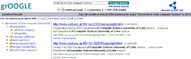
Figure 4: Results page

Table 12: Administration functionalities

$Modules$	$Functionalities$
Crawler	Starting points (seeds)
	Collection name
	Accept/Reject filetype list
	Maximum downloaded pages
	Host/Domain spanning
	Traversal algorithm
	Maximum crawling depth
	Repository path
	Configuration file path
	Logging (file path, log level)
	Re-crawling time period
Indexer	Create index
	Drop index
	Create new collection
Clustering	Algorithm used
	Number of clusters
	Maximum number of documents to be clustered
	Max/min title length for clusters
	Maximum depth for cluster tree
	Name hierarchy for cluster tree
	Minimum documents in clusters
	Maximum number of words in each document
Taxonomy	Number of levels
	Number of output levels
Query Expansion	Enable/Disable
	Number of relevant documents
	Number of relevant words
Query Evaluator	Edit distance tolerance

3.12 Administration

This module glues together the various components and offers to the administrator of the web search engine a Web-based user interface for controlling its behavior, quickly and easily. Supported functionalities are listed in Table 12.

4 Comparison with Other Systems

Mitos offers a really wide spectrum of functionalities. Just indicatively, Table 13 lists the features that Mitos and some well known IR systems and web search engines offer.

Table 13: System & Functionalities Matrix

Functionality	Mitos	google	Terrier v.1.1	Vivisimo	Yahoo!	Lucene	Lemur
Crawler	$\checkmark$	$\checkmark$	$\checkmark$	$\checkmark$	$\checkmark$	$\times$	$\times$
Greek Stemmer	$\checkmark$	$\times$	$\times$	$\times$	$\times$	$\times$	$\times$
Result Clustering	$\checkmark$	$\times$	$\times$	$\checkmark$	$\times$	$\times$	$\checkmark$
Edit Distance	$\checkmark$	$\checkmark$	$\times$	$\times$	$\checkmark$	$\times$	$\times$
Query Expansion	$\checkmark$	$\times$	$\checkmark$	$\times$	$\checkmark$	$\checkmark$	$\checkmark$
Link Analysis	$\checkmark$	$\checkmark$	$\times$	$\times$	$\checkmark$	$\times$	$\checkmark$
Several Retrieval Models	$\checkmark$	$\times$	$\checkmark$	$\times$	$\times$	$\times$	$\checkmark$

4.1 Indexing Performance

We compared the indexing mechanisms of Mitos and Terrier version 1.1 using our collection (the one described in Section 3). The entire collection is approximately 2.8 GB. Block addressing and debug message printing were disabled in both tools. Stemming and stop-words removal were also disabled in Mitos. The results of the comparison are shown in Table 14. Notice that the number of documents indexed by the two tools is not the same. Mitos managed to index more documents than Terrier due to its better file type identification technique. The files that Mitos failed to index are executables and media files, constituting only the 3.8% of the collection.

Regarding index size, the index of Terrier is about 8 times smaller than that of Mitos. Recall that Mitos uses a DBMS, while Terrier uses compression and special data structures. Nevertheless, the index size of Mitos is less than the 10% of the collection’s size. The size may increase in the future, if we decide to use the SP-GiST trie, since the B+-trees scale better with respect to index size according to [7].

On the other hand, Mitos offers faster index creation: it takes less than 1 hour to index about 2.8 GB of documents and is about four times faster than Terrier. In the future we will try to reproduce our findings with an updated Terrier version.

Table 14: Comparison of Indexing Techniques

$Tool$	$Index\ Size$	$Documents\ Indexed$	$Time$
Terrier v.1.1	23.8 MB (0.8%)	11699 (80.6%)	11694 sec
Mitos	214.99 MB (7.4%)	14246 (97.2%)	2892 sec

4.2 Searching Performance

Table 15 reports query evaluation times. These query evaluation times were calculated using the previously described collection of $N$=14246 documents with a vocabulary size of $|$V$|$=220518.

Table 15: Query Evaluation Times

Model	q	$|$ans(q)$|$	Time
Vector	csd math	1449	79 ms
Boolean	csd or math	1449	58 ms
Extended Boolean	csd or math	1449	187ms
Fuzzy	csd or math	1449	165 ms
Vector	information retrieval systems	6329	315 ms
Boolean	information or retrieval or systems	6329	260 ms
Extended Boolean	information or retrieval or systems	6329	522 ms
Fuzzy	information or retrieval or systems	6329	557 ms

Table 16 compares the evaluation times and results of Mitos and Terrier, using the Vector Space model and the collection previously described. 100 random queries were executed on both engines and average times were calculated. The process was repeated for 1 up to 10 random query terms. The modulus of the average difference in the number of the results was also calculated for each case.

Terrier offers constant searching times, regardless of terms number in the query and much higher performance than Mitos (due to the not optimized and DBMS nature of Mitos). On the other hand Mitos times increase monotonically with the number of terms in the query. Note the difference in the results number, a consequence of the bigger number of documents indexed by Mitos.

Table 16: Average Evaluation Times and Result Differences for 100 Iterations

$Query\ Terms\ Num.$	$\textit{{Mitos}}\ Avg.\ Time$	$Terrier\ Avg.\ Time$	$|Result\ Avg.\ Diff.|$
1	0.0690	0.0018	2.35
2	0.1598	0.0020	10.01
3	0.1540	0.0022	14.94
4	0.1741	0.0014	7.12
5	0.2016	0.0016	28.79
6	0.2005	0.0018	52.4
7	0.2434	0.0018	78.24
8	0.2714	0.0014	5.16
9	0.3284	0.0017	56.71
10	0.3212	0.0044	90.23

5 Summary and Concluding Remarks

There are only few concise papers (e.g. [1]) that discuss all aspects revolving the design, implementation and evaluation of Web search engines. This paper presented a brief description of Mitos, a currently developed web search engine offering a wide spectrum of functionalities including an advanced stemmer for the Greek language and real-time result clustering. Another distinctive characteristic of Mitos is that its index is based on a DBMS. For this reason, we have discussed issues regarding the usage of DBMSs for managing the index and we have compared our engine with other engines whose index is not based on a DBMS. In brief, the DBMS-based index requires more storage space and offers poorer performance (as expected), but on the other hand it is more extensible. In addition:

• we realized that stemming has a number of benefits (improves recall, reduces the size of the index), but affects negatively the selection of the best text (that is used for creating document surrogates), the quality (readability) of the cluster names, and the quality of the suggested terms (during query expansion),

• we verified that the distribution of words approximates a power-law distribution,

• we realized that result clustering is a hard problem that is worth further research.

In future, we plan to

• conduct experiments with larger collections.

• extend the crawler so that to support important-first-traversal (also taking into account the rank field in the db).

• continue improving the real-time results clustering module

• investigate PostgreSQL indices that offer better performance for indexing and query evaluation.

• reproduce indexing times with an updated version of Terrier and a bigger documents collection.

References

- [1] A. Arasu, J. Cho, H. Garcia-Molina, A. Paepcke, and S. Raghavan. Searching the Web. ACM Transactions on Internet Technology, 1(1):2–43, 2001.
- [2] Walid Aref, Daniel Barbará, and Padmavathi Vallabhaneni. The handwritten trie: indexing electronic ink. SIGMOD Rec., 24(2):151–162, 1995.
- [3] Walid G. Aref and Ihab F. Ilyas. Sp-gist: An extensible database index for supporting space partitioning trees. J. Intell. Inf. Syst., 17(2-3):215–240, 2001.
- [4] Ricardo Baeza-Yates and Berthier Ribeiro-Neto. “Modern Information Retrieval”. ACM Press, Addison-Wesley, 1999.
- [5] Sergey Brin and Lawrence Page. “The Anatomy of a Large-scale Hypertextual Web Search Engine”. In Proceedings of the 7th International WWW Conference, Brisbane, Australia, April 1998.
- [6] Deepayan Chakrabarti and Christos Faloutsos. Graph mining: Laws, generators, and algorithms. ACM Comput. Surv., 38(1), 2006.
- [7] Mohamed Y. Eltabakh, Ramy Eltarras, and Walid G. Aref. Space-partitioning trees in postgresql: Realization and performance. In ICDE ’06: Proceedings of the 22nd International Conference on Data Engineering (ICDE’06), page 100, Washington, DC, USA, 2006. IEEE Computer Society.
- [8] M.Y. Eltabakh, W.G. Aref, and R. Eltarras. To trie or not to trie? realizing space-partitioning trees inside postgresql: Challenges, experiences and performance. Technical Report TR-05-008, Department of Computer Science, Purdue University, USA, April 2005.
- [9] Ntais G. Development of a stemmer for the greek language. Master’s thesis, Department of Computer and Systems Sciences, Stockholm University / Royal Institute of Technology, Sweden, 2006.
- [10] Zoltan Gyongyi, Hector Garcia-Molina, and Jan Pedersen. “Combating Web Spam with TrustRank”. In Procs. of the 30th Intern. Conference on Very Large Data Bases, VLDB’2004, Toronto, Canada, August 2004.
- [11] David A. Hull. Stemming algorithms: A case study for detailed evaluation. Journal of the American Society of Information Science, 47(1):70–84, 1996.
- [12] Preslav Nakov. Design and evaluation of inflectional stemmer for bulgarian.
- [13] M. F. Porter. An algorithm for suffix stripping. pages 313–316, 1997.
- [14] W. H. Press, S. A. Teukolsky, W. T. Vetterling, and B. P. Flannery. Numerical Recipes in C. Cambridge University Press, 1992. (2nd edition).
- [15] Manolis Terrovitis, Spyros Passas, Panos Vassiliadis, and Timos Sellis. A combination of trie-trees and inverted files for the indexing of set-valued attributes. In CIKM ’06: Proceedings of the 15th ACM international conference on Information and knowledge management, pages 728–737, New York, NY, USA, 2006. ACM Press.