Forward-like functions for dual parametrization of GPDs from the nonlocal chiral quark model

Abstract

We derive the set of inversion relations allowing to establish the link between the dual parametrization of GPDs and a broad class of phenomenological models for GPDs. As an example we consider the results of the calculation of the pion GPD in the nonlocal chiral quark model (NlCQM) to recover the set of forward-like functions $Q_{2\nu}$ representing this GPD in the framework of dual parametrization. We also argue that Abel tomography method overlooks possible $\delta$-function like contributions to GPD quintessence function which make explicit contribution to the $D$-from factor.

1 Introduction

Generalized parton distributions (GPDs) pioneers have been in focus of intensive studies during the past decade. These distributions, which arise as natural generalization of parton distribution functions (PDFs) familiar from inclusive reactions, proved to be an extremely efficient tool for the description of hadron properties in terms of quark and gluonic degrees of freedom. Experimentally GPDs are accessed through hard exclusive reactions. Reviews of both theoretical and experimental aspects are given e.g. in refs GPV ; Diehl ; BelRad ; Boffi .

It is needless to say that the direct extraction of GPDs from the amplitudes of hard exclusive processes is highly demanded, since these functions contain a wealth of information on hadron structure. Unfortunately, the problem turns out to be very complicated, since GPDs depend on three variables ($x,\,\xi,\,t$) as well as on renormalization scale. Moreover, GPDs always enter the observable quantities (cross-sections, spin asymmetries etc.) as certain convolutions with perturbative kernels. All this makes the extraction of GPDs from the observables an extremely difficult task. As a palliative different models for GPDs are employed. These models should satisfy the requirements of polynomiality and positivity which are the consequences of general principles of Lorentz invariance and positivity of probability.

Historically the most popular model for GPDs is double distribution parametrization suggested by Radyushkin RadDDandEvolution . In this parametrization the GPD is given as a convolution of a forward parton distribution $q(\beta)$ with a specific profile function $h(\beta,\alpha)$:

$$\begin{split}&H^{q}(x,\xi,t=0)=\\ &\int_{-1}^{1}d\beta\int_{-1+|\beta|}^{1-|\beta|}d\alpha\,\delta(x-\beta-\alpha\xi)\,h(\beta,\alpha)q(\beta).\end{split}$$

This parametrization presents a simple and convenient form of GPDs and is used in numerous phenomenological applications. However, as was pointed out in Polyakov:1999gs , it does not satisfy the polynomiality condition in its full form. To overcome this problem one has to complete GPD in double parametrization with the so-called $D$-term.

A different elegant way to implement polynomiality of GPDs was proposed in Polyakov:2002wz . This alternative parametrization is called dual since it is based on the representation of GPDs as infinite series of $t$-channel exchanges. In this paper we discuss some properties of dual parametrization and derive the set of inversion relations allowing to establish the link between a broad class of phenomenological models of GPDs and the dual parametrization. As an example we consider the nonlocal chiral quark model for quark GPDs in a pion and with the help of the inversion formulas determine the shape of the corresponding forward-like functions $Q_{0}$, $Q_{2}$, $Q_{4}$. We compare these functions to the GPD quintessence function $N(x)$ calculated with the help of the method of Abel tomography Tomography . We also calculate the $D$-form factor as well as the first coefficient of Gegenbauer expansion of the $D$-term in the framework of nonlocal chiral quark model.

2 Basic facts on the dual parametrization of GPDs

Below we consider only the case of the singlet ($C=+1$) GPD for spin-$0$ target. In the forward limit this GPD is reduced to $\frac{1}{2}(q(x)+\bar{q}(x))$. The generalization for the nonsinglet ($C=-1$) GPD (the one reducing to $\frac{1}{2}(q(x)-\bar{q}(x))$ in the forward limit) is straightforward.

According to the result of Polyakov:1998ze , the partial wave decomposition in the $t$-channel for singlet GPD $H(x,\xi,t)$ can be written as the following formal series:

$$\begin{split}&H(x,\xi,t)=\\ &\sum_{n=1\atop\text{odd}}^{\infty}\sum_{l=0\atop\text{even}}^{n+1}B_{nl}(t)\,\theta\left(1-\frac{x^{2}}{\xi^{2}}\right)\left(1-\frac{x^{2}}{\xi^{2}}\right)C_{n}^{\frac{3}{2}}\left(\frac{x}{\xi}\right)P_{l}\left(\frac{1}{\xi}\right),\end{split}$$ (1)

where $C_{n}^{\frac{3}{2}}(\chi)$ stand for Gegenbauer polynomials; $P_{l}(\chi)$ are Legendre polynomials and $B_{nl}(t)$ are the generalized form factors; $x$, $\xi$ and $t$ stand for usual GPD variables.

The problem of summing up the formal series (1) was solved in Polyakov:2002wz . For this one has to introduce the set of forward-like functions $Q_{2\nu}(x,t)$ $(\nu=0,\,1,\,...)$ whose Mellin moments generate the generalized form factors $B_{nl}(t)$:

$$B_{n\,n+1-2\nu}(t)=\int_{0}^{1}dxx^{n}Q_{2\nu}(x,t)\,.$$ (2)

The set of forward-like functions $Q_{2\nu}(x,t)$ is connected to GPD $H(x,\xi,t)$ in dual parametrization with the help of the following relation:

$$\begin{split}&H(x,\xi,t)=\sum_{\nu=0}^{\infty}\left\{\frac{\xi^{2\nu}}{2}\left[H^{(\nu)}(x,\xi,t)-H^{(\nu)}(-x,\xi,t)\right]\,\right.\\ &-\left(1-\frac{x^{2}}{\xi^{2}}\right)\theta(\xi-|x|)\\ &\times\sum_{l=1\atop\text{odd}}^{2\nu-3}C_{2\nu-l-2}^{\frac{3}{2}}\left(\frac{x}{\xi}\right)\left.P_{l}\left(\frac{1}{\xi}\right)\int_{0}^{1}dyy^{2\nu-l-2}Q_{2\nu}(y,t)\right\}\,,\end{split}$$ (3)

where the functions $H^{(\nu)}(x,\xi,t)$ defined for $-\xi\leq x\leq 1$ are given by the following integral transformations:

$$\begin{split}H^{(\nu)}(x,\xi,t)&=\theta(x>\xi)\frac{1}{\pi}\int_{y_{0}}^{1}\frac{dy}{y}\left[\left(1-y\frac{\partial}{\partial y}\right)Q_{2\nu}(y,t)\right]\\ &\times\left.\int_{s_{1}}^{s_{2}}ds\,\frac{x_{s}^{1-{2\nu}}}{\sqrt{2x_{s}-x_{s}^{2}-\xi^{2}}}\right.\,+\\ &\theta(x<\xi)\frac{1}{\pi}\int_{0}^{1}\frac{dy}{y}\left[\left(1-y\frac{\partial}{\partial y}\right)Q_{2\nu}(y,t)\right]\\ &\times\left.\int_{s_{1}}^{s_{3}}ds\frac{x_{s}^{1-2\nu}}{\sqrt{2x_{s}-x_{s}^{2}-\xi^{2}}}\right.\,.\end{split}$$ (4)

Here $x_{s}=2\frac{x-\xi s}{(1-s^{2})y}$. $s_{i}$, ($i=1,...\,4$) stand for the four roots of the equation $2x_{s}-x_{s}^{2}-\xi^{2}=0$ given by the following expressions:

$$\begin{split}&s_{1}=\frac{1}{y}\left(\mu-\sqrt{\left(1-x\,y\right)\,\left(1+{\mu}^{2}\right)-(1-y^{2})}\right);\\ &s_{2}=\frac{1}{y}\left(\mu+\sqrt{\left(1-x\,y\right)\,\left(1+{\mu}^{2}\right)-(1-y^{2})}\right);\\ &s_{3}=\frac{1}{y}\left(\lambda-\sqrt{\left(1-x\,y\right)\,\left(1+{\lambda}^{2}\right)-(1-y^{2})}\right);\\ &s_{4}=\frac{1}{y}\left(\lambda+\sqrt{\left(1-x\,y\right)\,\left(1+{\lambda}^{2}\right)-(1-y^{2})}\right),\end{split}$$

where we have introduced the notations:

$$\mu=\frac{1-\sqrt{1-\xi^{2}}}{\xi};\ \ \ \ \lambda=\frac{1}{\mu}\;.$$

$y=y_{0}$ and $y=\frac{1}{y_{1}}$ are two solutions of the equation: $s_{1}=s_{2}$:

$$y_{0}=\frac{x\,\left(1+{\mu}^{2}\right)}{2}+{\sqrt{\frac{x^{2}\,{\left(1+{\mu}^{2}\right)}^{2}}{4}-{\mu}^{2}}};$$

$$y_{1}=\frac{x\,\left(1+{\lambda}^{2}\right)}{2}+{\sqrt{\frac{x^{2}\,{\left(1+{\lambda}^{2}\right)}^{2}}{4}-{\lambda}^{2}}}.$$

Here we give a short summary of the main features of dual parametrization approach:

• Once dual parametrization is used the corresponding GPD satisfies all general constrains such as the forward limit and the polynomiality condition in their full form.

• At the leading order the scale dependence of forward-like functions $Q_{2\nu}(x,t)$ is given by the usual DGLAP evolution equation.

• The forward-like function $Q_{0}(x,t=0)\equiv Q_{0}(x)$ is expressed through the singlet forward parton distribution $q(x)+\bar{q}(x)$ as:

  $$Q_{0}(x)=q(x)+\bar{q}(x)-\frac{x}{2}\int_{x}^{1}\frac{dy}{y^{2}}\,(q(y)+\bar{q}(y)).$$ (5)

• The basic mechanical characteristics of a hadron (hadron momentum and angular momentum fractions carried by quarks, radial distribution of forces experienced by quarks in a hadron) are contained in the lowest forward-like functions $Q_{0}(x)$, $Q_{2}(x)$.

3 GPD quintessence and Abel tomography

The amplitudes of hard exclusive processes are given by the convolutions of GPDs with the perturbative kernel. The leading order DVCS amplitude can be expressed through the corresponding elementary amplitude:

$$A(\xi,t)=\int_{0}^{1}dxH(x,\xi,t)\left[\frac{1}{\xi-x-i\epsilon}-\frac{1}{\xi+x-i\epsilon}\right]\,.$$ (6)

In the framework of dual parametrization of GPDs it turns out possible to specify what part of information on GPDs can be reconstructed from the known amplitudes of hard exclusive processes. In Tomography the explicit formulae relating the special combination of forward-like functions $Q_{2\nu}$ to the amplitude of hard exclusive process were derived.

The crucial role in this issue is played by the so-called GPD quintessence function Tomography ; Polyakov:2007rw ; Polyakov:2008xm :

$$N(x,t)=\sum_{\nu=0}^{\infty}x^{2\nu}Q_{2\nu}(x,t)\,.$$

GPD quintessence function is of particular importance since, according to the result of Tomography , the real and the imaginary parts of the standard amplitude (6) are expressed in terms of this function:

$$\text{Im}A(\xi,t)=\int_{\frac{1-\sqrt{1-\xi^{2}}}{\xi}}^{1}\frac{dx}{x}\,N(x,t)\left[\frac{1}{\sqrt{\frac{2x}{\xi}-x^{2}-1}}\right]\,;$$ (7)

$$\begin{split}&\text{Re}A(\xi,t)=2D(t)+\int_{0}^{\frac{1-\sqrt{1-\xi^{2}}}{\xi}}\frac{dx}{x}\,N(x,t)\times\\ &\left[\frac{1}{\sqrt{1-\frac{2x}{\xi}+x^{2}}}+\frac{1}{\sqrt{1+\frac{2x}{\xi}+x^{2}}}-\frac{2}{\sqrt{1+x^{2}}}\right]+\\ &\int_{\frac{1-\sqrt{1-\xi^{2}}}{\xi}}^{1}\frac{dx}{x}\,N(x,t)\left[\frac{1}{\sqrt{1+\frac{2x}{\xi}+x^{2}}}-\frac{2}{\sqrt{1+x^{2}}}\right]\,.\end{split}$$ (8)

Here $D(t)$ stands for the so-called $D$-form factor which actually is the subtraction constant in the dispersion relation in $\xi$ plane for the amplitude $A(\xi,t)$ Anikin:2007yh ; Diehl:2007ru . The following expression for the $D$-form factor was derived in Tomography :

$$\begin{split}D(t)=&\int_{0}^{1}\frac{dx}{x}Q_{0}(x,t)\left(\frac{1}{\sqrt{1+x^{2}}}-1\right)+\\ &\int_{0}^{1}\frac{dx}{x}\left[N(x,t)-Q_{0}(x,t)\right]\frac{1}{\sqrt{1+x^{2}}}\,.\end{split}$$ (9)

Moreover, the GPD quintessence function $N(x,t)$ can be recovered from the known imaginary part of the amplitude (6). The corresponding procedure was described in Tomography ; Moiseeva:2008qd . With the help of Joukowski conformal map it turns out possible to present the relation between the imaginary part of the amplitude and $N(x,t)$ (7) in the form of the so-called Abel integral equation Moiseeva:2008qd . This equation can be easily inverted yielding the following relation for $N(x,t)$ Tomography :

$$\begin{split}N(x,t)=&\frac{2}{\pi}\,\frac{x(1-x^{2})}{(1+x)^{\frac{3}{2}}}\int_{\frac{2x}{1+x^{2}}}^{1}\frac{d\xi}{\xi^{\frac{3}{2}}}\frac{1}{\sqrt{\xi-\frac{2x}{1+x^{2}}}}\times\\ &\left\{\frac{1}{2}\text{Im}A(\xi,t)-\xi\frac{d}{d\xi}\text{Im}A(\xi,t)\right\}\,.\end{split}$$ (10)

Thus the information on GPD which can be recovered from the amplitude of a hard exclusive process (at fixed hard scale) is encoded in the GPD quintessence function $N(x,t)$ and the value of $D$-form factor $D(t)$. The formula (10) allows to restore GPD quintessence function $N(x,t)$ for $x\neq 0$ from the measured imaginary part of the amplitude. In what follows we are going to show that $N(x,t)$ may obtain additional $\delta$-function like contributions having a support at $x=0$ which are overlooked by Abel tomography procedure described above. These contributions affect the value of $D$-form factor giving additional contribution to (9).

4 Polynomiality and the $D$-term

The polynomiality condition for Mellin moments of the generalized parton distribution implies that pioneers :

$$\begin{split}&\int_{-1}^{1}dx\,x^{N}H(x,\xi,t)=\\ &h_{0}^{(N)}(t)+h_{2}^{(N)}(t)\xi^{2}+...+h_{N+1}^{(N)}(t)\xi^{N+1}\ \ \ (N-\text{odd})\,.\end{split}$$ (11)

In the framework of the dual parametrization the set of coefficients $h_{k}^{(N)}$ can be calculated from the partial wave decomposition of Mellin moments that follows from (1) Polyakov:1998ze :

$$\begin{split}&\int_{-1}^{1}dx\,x^{N}H(x,\xi,t)=\xi^{N+1}\sum_{n=1\atop\text{odd}}^{N}\sum_{l=0\atop\text{even}}^{n+1}B_{nl}(t)P_{l}\left(\frac{1}{\xi}\right)\times\\ &\frac{\Gamma(\frac{3}{2})\Gamma(N+1)(n+1)(n+2)}{2^{N}\Gamma(\frac{N-n}{2}+1)\Gamma(\frac{N+n}{2}+\frac{5}{2})}\ \ \ (N-\text{odd})\,.\end{split}$$ (12)

Hence, for even $k\leq N+1$:

$$\begin{split}&h_{k}^{(N)}(t)=\sum_{n=1\atop\text{odd}}^{N}\sum_{l=0\atop\text{even}}^{n+1}B_{nl}(t)\frac{1}{(N+1-k)!}P_{l}^{(N+1-k)}\left(0\right)\times\\ &\frac{\Gamma(\frac{3}{2})\Gamma(N+1)(n+1)(n+2)}{2^{N}\Gamma(\frac{N-n}{2}+1)\Gamma(\frac{N+n}{2}+\frac{5}{2})}\,.\end{split}$$ (13)

A special attention is to be payed to the coefficients $h^{(N)}_{N+1}$ which are generated by the so-called $D$-term Polyakov:1999gs . An important advantage of dual parametrization of GPDs comparing e.g. to double distribution parametrization is that the $D$-term is its natural ingredient. The coefficients $d_{n}(t)$ of the Gegenbauer expansion of the $D$-term

$$\begin{split}&D(z,t)=\\ &(1-z^{2})\left[d_{1}(t)C_{1}^{\frac{3}{2}}(z)+d_{3}(t)C_{3}^{\frac{3}{2}}(z)+d_{5}(t)C_{5}^{\frac{3}{2}}(z)+...\right]\,\end{split}$$

can be computed with the help of the following generating function Tomography :

$$\begin{split}\sum_{n=1\atop\text{odd}}^{\infty}&d_{n}(t)\alpha^{n}=\\ &\frac{1}{\alpha}\int_{0}^{1}\frac{dz}{z}\sum_{\nu=0}^{\infty}(\alpha z)^{2\nu}Q_{2\nu}(z,t)\left(\frac{1}{\sqrt{1+\alpha^{2}z^{2}}}-\delta_{\nu 0}\right).\end{split}$$

Let us now assume that a certain additional artificial $D$-term $\theta(1-\frac{x^{2}}{\xi^{2}})\,\delta{D}\left(\frac{x}{\xi},t\right)$ is appended to GPD $H(x,\xi,t)$. $\delta{D}(z,t)$ is supposed to be an arbitrary odd function with respect to variable $z$ having the support $-1\leq z\leq 1$. Its Gegenbauer expansion reads:

$$\delta{D}(z,t)=(1-z^{2})\sum_{n=1\atop\text{odd}}^{\infty}\delta{d}_{n}(t)\,C_{n}^{\frac{3}{2}}(z).$$ (14)

In the Mellin moments the $D$-term contributes only to the highest power of $\xi$:

$$\begin{split}&\int_{-1}^{1}dx\,x^{N}\theta\left(1-\frac{x^{2}}{\xi^{2}}\right)\,\delta{D}\left(\frac{x}{\xi},t\right)=\\ &\xi^{N+1}\sum_{n=1\atop\text{odd}}^{N}\delta{d}_{n}(t)\frac{\Gamma(\frac{3}{2})\Gamma(N+1)(n+1)(n+2)}{2^{N}\Gamma(\frac{N-n}{2}+1)\Gamma(\frac{N+n}{2}+\frac{5}{2})}\,.\end{split}$$ (15)

The $D$-term contribution to the $N$-th Mellin moment (15) can be incorporated into the general form (12) employed in the framework of dual parametrization with the help of the following change of the form factors $B_{(2\nu-1)\,0}=\int_{0}^{1}dxx^{2\nu-1}Q_{2\nu}(x)$ ($\nu\geq 1$):

$$\begin{split}&B_{(2\nu-1)\;0}(t)\longrightarrow B_{(2\nu-1)\;0}(t)+\delta{d}_{2\nu-1}(t);\\ &Q_{2\nu}(x,t)\longrightarrow Q_{2\nu}(x,t)-\delta{d}_{2\nu-1}(t)\frac{2}{(\nu-1)!}\,\delta^{(2\nu-1)}(x);\end{split}$$ (16)

Hence we can conclude that:

• The initial implicit assumption of dual parametrization approach that the functions $Q_{2\nu}(x,t)$ belong to the class of smooth functions seems to be too restrictive.

• Instead one has to consider the functions $Q_{2\nu}(x,t)$ with $\nu>0$ as generalized functions. In fact this is quite natural since the functions $Q_{2\nu}$ are not directly measurable. The physical (observable) quantities are always expressed through Mellin convolutions of forward-like functions $Q_{2\nu}(x,t)$.

Let us now turn to the GPD quintessence function $N(x,t)$. Once the $\delta{D}(t)$ term is added to GPD $N(x,t)$ receives additional singular contribution with the point-like support:

$$\delta{N}(x,t)=-\sum_{n=1\atop\text{odd}}^{\infty}x^{n+1}\,\delta{d}_{n}(t)\frac{2}{n!}\,\delta^{(n)}(x)\,.$$ (17)

Clearly the non-zero contribution to observable quantities may come only from the convolution of $\delta N(x)$ with a kernel having a $1/x$ singularity at $x=0$. Hence (17) does not affect the value of $\text{Im}A(\xi,t)$. This means that the presence of the contribution of the type (17) can not be revealed with the help of the method of Abel tomography. As for the real part of the amplitude one can check that the convolution of $\delta{N}(x,t)$ with the kernel singular at $x=0$ appearing in second item of (9) results in the explicit contribution to the $D$-form factor.

Thus, in variance with statement of Tomography ; Polyakov:2007rw , we conclude that the correct value of the $D$-form factor can not be computed just from known $Q_{0}(x,t)$ and $N(x,t)$ recovered with the help of Abel tomography method (10) since this method overlooks the singular contributions of type (17). The missing information on the $D$-form factor can be obtained from the direct measurement of the real part of the amplitude.

Let us also point that the singular contribution (17) does not alter the value of $J$ ($J>0$) Mellin moments of GPD quintessence function which, according to the result of Tomography , Polyakov:2007rw are related to the contributions of states with fixed angular momentum in $t$-channel:

$$\int_{0}^{1}dx\,x^{J-1}N(x,t)=\frac{1}{2}\int_{-1}^{1}dz\,\frac{\Phi_{J}(z,t)}{1-z}.$$ (18)

Here $\Phi_{J}(z,t)$ stands for the distribution amplitude corresponding to two quark exchange in the $t$-channel with fixed angular momentum $J$.

5 On the expansion of GPD around $\xi=0$ to the order $\xi^{4}$

Starting from (4) one can construct the systematic expansion of the GPD $H(x,\xi,t)$ in powers of small $\xi$ for the fixed value of $x>\xi$. In Tomography such an expansion was constructed to the order $\xi^{2}$. Here we present the result up to the order $\xi^{4}\,$. According to (3) for $x>\xi$ ($\xi\geq 0$):

$$\begin{split}&H(x,\xi,t)=\\ &\frac{1}{2}\,H^{(0)}(x,\xi,t)+\frac{1}{2}\,\xi^{2}H^{(1)}(x,\xi,t)+\frac{1}{2}\,\xi^{4}H^{(2)}(x,\xi,t)+...\end{split}$$ (19)

The result for $H^{(0)}(x,t)$ up to the order $\xi^{4}$ reads:

$$\begin{split}&H^{(0)}(x,\xi,t)=Q_{0}(x,t)+\frac{\sqrt{x}}{2}\int_{x}^{1}\frac{dy}{y^{\frac{3}{2}}}Q_{0}(y,t)+\\ &\xi^{2}\left[\frac{x^{2}-1}{4x}\frac{\partial}{\partial x}Q_{0}(x,t)+\right.\\ &\left.\frac{1}{32}\int_{x}^{1}dyQ_{0}(y,t)\left\{\frac{1}{y}\left(3\,{\sqrt{\frac{x}{y}}}+3\,{\sqrt{\frac{y}{x}}}\right)+\right.\right.\\ &\left.\left.\frac{1}{y^{3}}\left(3\,{\sqrt{\frac{y}{x}}}-{\left(\frac{y}{x}\right)}^{\frac{3}{2}}\right)\right\}\right]+\\ &\xi^{4}\left[-\frac{(1-x^{2})(9x^{2}+3)}{64x^{3}}\frac{\partial}{\partial x}Q_{0}(x,t)\right.+\\ &\frac{2x(1-x^{2})^{2}}{64x^{3}}\frac{\partial^{2}}{\partial x^{2}}Q_{0}(x,t)+\\ &\frac{1}{64}\int_{x}^{1}dyQ_{0}(y,t)\left.\left\{\frac{1}{y}\left(\frac{105}{32}{\sqrt{\frac{x}{y}}}+\frac{45}{16}{\sqrt{\frac{y}{x}}}+\frac{45}{32}{\left(\frac{y}{x}\right)}^{\frac{3}{2}}\right)+\right.\right.\\ &\left.\left.\frac{1}{y^{3}}\left(\frac{45}{16}{\sqrt{\frac{y}{x}}}-\frac{3}{8}{\left(\frac{y}{x}\right)}^{\frac{3}{2}}+\frac{9}{16}{\left(\frac{y}{x}\right)}^{\frac{5}{2}}\right)+\right.\right.\\ &\left.\left.\frac{1}{y^{5}}\left(\frac{45}{32}{\left(\frac{y}{x}\right)}^{\frac{3}{2}}+\frac{9}{16}{\left(\frac{y}{x}\right)}^{\frac{5}{2}}-\frac{15}{32}{\left(\frac{y}{x}\right)}^{\frac{7}{2}}\right)\right\}\right]+O(\xi^{6})\,.\end{split}$$ (20)

The result for $H^{(1)}(x,\xi,t)$ to the order $\xi^{2}$ reads:

$$\begin{split}&H^{(1)}(x,\xi,t)=\frac{1}{4}Q_{2}(x,t)+\\ &\frac{3}{32}\int_{x}^{1}dyQ_{2}(y,t)\frac{1}{y}\left(\frac{1}{2}{\sqrt{\frac{x}{y}}}+{\sqrt{\frac{y}{x}}}+\frac{5}{2}{\left(\frac{y}{x}\right)}^{\frac{3}{2}}\right)+\\ &\xi^{2}\left[\frac{1+x^{2}}{16x^{2}}Q_{2}(x,t)-\frac{1-x^{2}}{16x}\frac{\partial}{\partial x}Q_{2}(x,t)+\right.\\ &\left.\frac{1}{1024}\int_{x}^{1}dyQ_{2}(y,t)\times\right.\\ &\left.\left\{\frac{1}{y}\left(35\,{\sqrt{\frac{x}{y}}}+45\,{\sqrt{\frac{y}{x}}}+45\,{\left(\frac{y}{x}\right)}^{\frac{3}{2}}+35\,{\left(\frac{y}{x}\right)}^{\frac{5}{2}}\right)+\right.\right.\\ &\left.\left.\frac{1}{y^{3}}\left(15\,{\sqrt{\frac{y}{x}}}-3\,{\left(\frac{y}{x}\right)}^{\frac{3}{2}}+9\,{\left(\frac{y}{x}\right)}^{\frac{5}{2}}+75\,{\left(\frac{y}{x}\right)}^{\frac{7}{2}}\right)\right\}\right]+\\ &O(\xi^{4})\,.\end{split}$$ (21)

Finally the result for $H^{(2)}(x,\xi,t)$ to the order $\xi^{0}$ reads:

$$\begin{split}&H^{(2)}(x,\xi,t)=\frac{1}{16}Q_{4}(x,t)+\frac{5}{1024}\int_{x}^{1}dy\,Q_{4}(y,t)\frac{1}{y}\times\\ &\left(\frac{7}{4}{\sqrt{\frac{x}{y}}}+3\,{\sqrt{\frac{y}{x}}}+\frac{9}{2}{\left(\frac{y}{x}\right)}^{\frac{3}{2}}+7\,{\left(\frac{y}{x}\right)}^{\frac{5}{2}}+\frac{63}{4}{\left(\frac{y}{x}\right)}^{\frac{7}{2}}\right)+\\ &O(\xi^{2})\,.\end{split}$$ (22)

Several notes are in order:

• One can check that exactly the same expansion is valid for non-singlet ($C=-1$) GPDs. Clearly in this case one has to use the set of non-singlet forward-like functions.

• An important property of the expansion of the GPD in powers of $\xi$ (19), (20), (21), (22) is that up to the particular order $\xi^{2\mu}$ it involves only a finite number of functions $Q_{2\nu}(x)$ with $\nu\leq\mu$ (e.g. to the order $\xi^{4}$ only $Q_{0}$, $Q_{2}$ and $Q_{4}$ are relevant). This allows to invert this expansion and to express the set of functions $Q_{2\nu}$ through GPDs for various phenomenological parametrizations of GPDs. This problem is addressed in the next Section.

• Let us assume the small $x$ behavior for the forward-like functions to be the following: $Q_{2\nu}(x)\sim\frac{1}{x^{2\nu+\alpha}}$, where the power $\alpha$ governs the small $x$ behavior of forward quark distribution ($\alpha<2$). Then with the help of explicit calculation one can check that the $N$-th Mellin moments of the appropriate coefficients of small $\xi$ expansion (19) will produce the values of $h_{k}^{(N)}$ for $k\leq N-1$ coinciding with those obtained from (13). However, the result for the coefficient at the highest power of $\xi$ of $N$-th Mellin moment $h_{N+1}^{(N)}$ obtained from the expansion (19) does not coincide with the value (13) if $\alpha\geq 0$.

6 Expressions for forward-like functions

Let us assume that the expansion of the singlet (or nonsinglet) GPD $H(x,\xi)\equiv H(x,\xi,t=0)$ around $\xi=0$ for $x>\xi$ calculated in the framework of a certain model is known:

$$H(x,\xi)=\phi_{0}(x)+\phi_{2}(x)\xi^{2}+\phi_{4}(x)\xi^{4}+O(\xi^{6})\,.$$ (23)

Here

$$\phi_{2\nu}(x)=\frac{1}{(2\nu)!}\,\frac{\partial^{2\nu}}{\partial\xi^{2\nu}}\,H(x,\xi)_{\xi=0}\,.$$

Using this expansion together with (19) one can try to determine the corresponding functions $Q_{2\nu}(x,t=0)\equiv Q_{2\nu}(x)$ from order to order.

Let us start with the function $Q_{0}$. Clearly, since the GPD calculated in the realistic model has the correct forward limit

$$\phi_{0}(x)\equiv H(x,\xi=0)=\frac{q(x)}{2}\,.$$

Here $q(x)$ stands for either for singlet (quark plus antiquark) or nonsinglet (quark minus antiquark) combination of forward quark distributions. Hence for $Q_{0}(x)$ we get

$$q(x)=Q_{0}(x)+\frac{\sqrt{x}}{2}\int_{x}^{1}\frac{dy}{y}\frac{1}{\sqrt{\,y}}\,Q_{0}(y)$$

and after inverting it we recover the usual expression for $Q_{0}(x)$:

$$Q_{0}(x)=q(x)-\frac{x}{2}\int_{x}^{1}\frac{dy}{y^{2}}\,q(y)\,.$$ (24)

Let us now consider a more involved case. In order to express $Q_{2}(x)$ one has to invert the following Mellin convolution:

$$Q_{2}(x)+\frac{3}{8}\int_{x}^{1}\frac{dy}{y}\left(\frac{1}{2}\sqrt{\frac{x}{y}}+\sqrt{\frac{y}{x}}+\frac{5}{2}\left(\frac{y}{x}\right)^{\frac{3}{2}}\right)Q_{2}(y)=f_{2}(x),$$ (25)

where $f_{2}(x)$ is determined by the $O(\xi^{2})$ term of expansion (23) minus the known $O(\xi^{2})$ contribution of $Q_{0}(x)$. Let $M_{2\;N}$ and $f_{2\;N}$ denote $N$-th Mellin moments of $Q_{2}$ and $f_{2}$ respectively:

$$\int_{0}^{1}dxx^{N}Q_{2}(x)=M_{2\;N};\ \ \ \ \int_{0}^{1}dxx^{N}f_{2}(x)=f_{2\;N}.$$

Then the relation between the $N$-th Mellin moments ($N>0$) of l.h.s. and r.h.s. of equation (25) reads:

$$M_{2\;N}\left(1+\frac{3}{8}\frac{8(1+6N+4N^{2})}{(-3-2N+12N^{2}+8N^{3})}\right)=f_{2\;N}\,.$$ (26)

The relation (26) can be easily inverted yielding the following expression for the forward-like function $Q_{2}(x)$:

$$Q_{2}(x)=f_{2}(x)-\int_{x}^{1}dyf_{2}(y)\left(\frac{15\,x}{16\,y^{2}}+\frac{3}{8\,y}+\frac{3}{16\,x}\right).$$

Now using the explicit expression for $f_{2}(x)$ we obtain the following result for $Q_{2}(x)$:

$$\begin{split}&Q_{2}(x)=\frac{2(1-x^{2})}{x^{2}}\,q(x)+\frac{(1-x^{2})}{x}\,q^{\prime}(x)+\\ &\int_{x}^{1}dy\,q(y)\left(\frac{-15\,x}{4\,y^{4}}-\frac{3}{2\,y^{3}}+\frac{5\,x}{4\,y^{2}}\right)+\\ &8\phi_{2}(x)-\int_{x}^{1}dy\,\phi_{2}(y)\left(\frac{15\,x}{2\,y^{2}}+\frac{3}{y}+\frac{3}{2\,x}\right).\end{split}$$ (27)

In the same manner we can derive the equation for $Q_{4}(x)$:

$$\begin{split}&Q_{4}(x)=f_{4}(x)-\\ &\int_{x}^{1}dyf_{4}(y)\left(\frac{35}{256}\frac{y^{2}}{x^{3}}+\frac{15}{64}\frac{y}{x^{2}}+\frac{45}{128}\frac{1}{x}+\frac{35}{64}\frac{1}{y}+\frac{315}{256}\frac{x}{y^{2}}\right)\,,\end{split}$$ (28)

where $f_{4}(x)$ is determined by the $O(\xi^{4})$ term of expansion (23) minus the known $O(\xi^{4})$ contribution of $Q_{0}(x)$ and $Q_{2}(x)$. Using the previously obtained results for $Q_{0}(x)$ and $Q_{2}(x)$ we derive the following explicit expression for $Q_{4}(x)$:

$$\begin{split}&Q_{4}(x)=\left(\frac{49}{8\,x^{4}}-\frac{17}{8\,x^{2}}\right)\,\left(1-x^{2}\right)q(x)+\\ &\left(\frac{7}{4\,x^{3}}-\frac{11}{4\,x}\right)\,\left(1-x^{2}\right)q^{\prime}(x)+\frac{{\left(1-x^{2}\right)}^{2}}{2\,x^{2}}q^{\prime\prime}(x)-\\ &\int_{x}^{1}dy\,q(y)\left(\frac{315\,x}{16\,y^{6}}+\frac{35}{4\,y^{5}}-\frac{135\,x}{8\,y^{4}}-\frac{21}{4\,y^{3}}+\frac{27\,x}{16\,y^{2}}\right)+\\ &\left(\frac{24}{x^{2}}-40\right)\phi_{2}(x)+\frac{8\,\left(1-x^{2}\right)}{x}\,\phi_{2}^{\prime}(x)-\\ &\int_{x}^{1}dy\phi_{2}(y)\left(\frac{315\,x}{8\,y^{4}}-\frac{7}{8\,x^{3}}+\frac{35}{2\,y^{3}}-\frac{135\,x}{4\,y^{2}}-\frac{21}{2\,y}-\frac{15}{4\,x}\right)+\\ &\frac{96}{3}\,\phi_{4}(x)-\\ &\int_{x}^{1}dy\,\phi_{4}(y)\left(\frac{45}{4\,x}+\frac{315\,x}{8\,y^{2}}+\frac{35}{2\,y}+\frac{15\,y}{2\,x^{2}}+\frac{35\,y^{2}}{8\,x^{3}}\right)\;.\end{split}$$ (29)

The expressions for $Q_{2\nu}$ with $\nu>2$ can be derived in a completely analogous way although they are very bulky. Thus we have described the reparametrization procedure in principle allowing to express any particular forward like function $Q_{2\nu}$ through GPD for a broad class of phenomenological models.

Note, that the starting point for the derivation of the expressions for $Q_{2\nu}(x)$ is the small $\xi$ expansion of $H(x,\xi)$ for $x>\xi$. Certainly this expansion is not affected when a $D$-term $\delta{D}\left(\frac{x}{\xi}\right)$ (14) is added to $H(x,\xi)$. Hence apart from the smooth part $Q_{2\nu}(x)$ with $\nu>0$ may obtain singular contributions of the type (16), which are certainly overlooked by the reparametrization procedure.

7 Pion GPDs calculated in the instanton-motivated effective chiral quark model

Now, in order to illustrate the application of the formalism discussed above, we are going to consider a certain specific model. As an example we have chosen the so-called instanton motivated effective quark model with non-local interactions Diakonov:1985eg (see Appendix A) allowing the calculation of pion distribution amplitude (DA), $2\pi$ DAs and pion GPDs at a low normalization point Petrov:1997ve ; Petrov:1998kg ; Polyakov:1998td ; Polyakov:1999gs ; Anikin:2000th ; Praszalowicz:2001pi ; Praszalowicz:2003pr .

The generalized parton distribution in a pion is defined as Fourier transform of the matrix element of quark light-cone operator taken between the pion states:

$$\begin{split}&\frac{1}{2}\int\frac{d\lambda}{2\pi}e^{i\lambda xn\cdot\bar{p}}\langle\pi^{b}(p^{\prime})|\bar{\psi}^{f^{\prime}}(-\frac{\lambda n}{2})\,{\hbox to0.0pt{/\hss}n}\,\psi^{f}(\frac{\lambda n}{2})|\pi^{a}(p)\rangle=\\ &\delta^{ab}\delta^{f^{\prime}f}H^{I=0}(x,\xi,t)+i\epsilon^{abc}(\tau^{c})^{f^{\prime}f}H^{I=1}(x,\xi,t).\end{split}$$ (30)

Here, as usual, $\bar{p}=\frac{p+p^{\prime}}{2}$; $\Delta=p^{\prime}-p$; $t=\Delta^{2}$. The skewness parameter is defined as $\xi=-\frac{\Delta^{+}}{2\bar{p}^{+}}$. $H^{I=0}(x,\xi,t)$ and $H^{I=1}(x,\xi,t)$ stand for isoscalar and isovector GPDs in a pion. In the forward limit these GPDs are reduced to the usual singlet (quark plus antiquark) and valence (quark minus antiquark) quark distributions respectively:

$$H^{I=0}(x,\xi=0,t=0)=\frac{1}{2}\left[q(x)+\bar{q}(x)\right],$$ (31)

$$H^{I=1}(x,\xi=0,t=0)=\frac{1}{2}\left[q(x)-\bar{q}(x)\right].$$ (32)

E.g. for $\pi^{+}$:

$$\begin{split}&H^{I=0}(x,\xi=0,t=0)=\\ &\begin{cases}&\frac{1}{2}\,[u^{\pi^{+}}(x)+\bar{u}^{\pi^{+}}(x)]\ \ \ \ \ \ \ \ \ \;\text{for}\;x>0\\ &\frac{1}{2}\,[-d^{\pi^{+}}(-x)-\bar{d}^{\pi^{+}}(-x)]\ \ \ \text{for}\;x<0\end{cases}\;.\end{split}$$ (33)

and

$$\begin{split}&H^{I=1}(x,\xi=0,t=0)=\\ &\begin{cases}&\frac{1}{2}\,[u^{\pi^{+}}(x)-\bar{u}^{\pi^{+}}(x)]\ \ \ \ \ \ \ \ \ \;\text{for}\;x>0\\ &\frac{1}{2}\,[-d^{\pi^{+}}(-x)+\bar{d}^{\pi^{+}}(-x)]\ \ \ \text{for}\;x<0\end{cases}\;.\end{split}$$ (34)

In the framework of the effective chiral quark model the isoscalar pion GPD obtains contributions from three diagrams presented on Fig 5, while the isovector one only from two first diagrams:

$$\begin{split}&H^{I=0}(x,\xi,t)=\mathcal{I}_{1}(x,\xi,t)+\mathcal{I}_{2}(x,\xi,t)+\mathcal{I}_{3}(x,\xi,t)\,;\\ &H^{I=1}(x,\xi,t)=\mathcal{I}_{1}(x,\xi,t)-\mathcal{I}_{2}(x,\xi,t)\,.\end{split}$$ (35)

One can check that $\mathcal{I}_{1}(x,\xi,t)$ is nonzero only if $-\xi\leq x\leq 1$; $\mathcal{I}_{3}(x,\xi,t)$ is nonzero only if $-\xi\leq x\leq\xi$;

$$\begin{split}&\mathcal{I}_{2}(x,\xi,t)=-\mathcal{I}_{1}(-x,\xi,t);\ \ \ \mathcal{I}_{3}(-x,\xi,t)=-\mathcal{I}_{3}(x,\xi,t)\\ &\mathcal{I}_{2}(x,-\xi,t)=\mathcal{I}_{1}(x,\xi,t);\ \ \ \mathcal{I}_{3}(x,-\xi,t)=\mathcal{I}_{3}(x,\xi,t)\end{split}$$ (36)

and hence $\mathcal{I}_{2}(-x,\xi,t)$ is nonzero only if $-1\leq x\leq\xi$.

Note that in the nonlinear chiral quark model

$$H^{I=0}(x,\xi,t)=\begin{cases}H^{I=1}(x,\xi,t)\ \ \ \text{for}\ \ \ x\geq\xi\\ -H^{I=1}(x,\xi,t)\ \ \ \text{for}\ \ \ x\leq-\xi\end{cases}\,.$$ (37)

Hence the result of calculation of forward like functions $Q_{2\nu}$ for the case of isovector quark GPD in a pion will be the same as that for isoscalar case. Thus in what follows we are going to consider the case of isoscalar quark GPD in a pion. For simplicity we set $t=0$, $m_{\pi}=0$. The explicit expression for the relevant contributions $\mathcal{I}_{1}$, $\mathcal{I}_{2}$, $\mathcal{I}_{3}$ are listed in the Appendix B.

On Fig. 1 we show the results of calculation of isoscalar quark GPD in a pion in the framework of nonlocal chiral quark model for $t=0$, $m_{\pi}=0$ and various values of $\xi$.

Figure 1: Quark isoscalar GPD calculated in the nonlocal chiral quark model (NlCQM) for various values of $\xi$. With the dashed line we show $H^{I=0}(x,\xi=0,t=0)\equiv\frac{1}{2}\left[q(x)+\bar{q}(x)\right]$.

8 Calculation of $Q_{2}(x)$ and $Q_{4}(x)$ and checking of the polynomiality condition

In this section we illustrate the application of the reparametrization procedure described in Sect. 6. Having in hands an analytic result (35), (B4) for quark isoscalar GPD in a pion $H(x,\xi)$ for $x\geq\xi$ calculated in the framework of non-local chiral quark model we can explicitly construct its small $\xi$ expansion for $x\geq\xi$ (23). Next with the help of (5), (27), (29) we can compute the forward-like functions $Q_{0}(x)$, $Q_{2}(x)$ and $Q_{4}(x)$. It is extremely instructive to compare these results to the general form of GPD quintessence function $N(x)$. This quantity also can be easily computed in the framework of chiral quark model.

In Fig. 2 we compare the results for $Q_{0}(x)$ (short-dashed line), $Q_{0}(x)+x^{2}Q_{2}(x)$ (long-dashed line), $Q_{0}(x)+x^{2}Q_{2}(x)+x^{4}Q_{4}(x)$ (thin solid line) calculated in the framework of nonlocal chiral quark model with the help of (5), (27), (29) to GPD quintessence function $N(x)$ reconstructed from the imaginary part of the DVCS amplitude (6) with the help of (10). On Fig. 3 we show the results for individual contributions of $Q_{0}(x)$, $Q_{2}(x)$ and $Q_{4}(x)$ functions into $N(x)$. It is interesting to note that in the case of nonlocal chiral quark model the functions $Q_{2\nu}(x)$ with higher $\nu$ provide only small corrections to the values of $N(x)$. In other words in the model under consideration the few first terms really dominate in the expansion of $N(x)$ into the sum of $x^{2\nu}Q_{2\nu}(x)$ induced by the inversion of small $\xi$ expansion of GPD. In fact the same conclusion remains valid in the case when Radyushkin DD-model is used as an input for the dual parametrization of GPDs (the corresponding analysis will be published elsewhere).

Figure 2: We compare our results for $Q_{0}(x)$ (short-dashes line), $Q_{0}(x)+x^{2}Q_{2}(x)$ (long-dashed line), $Q_{0}(x)+x^{2}Q_{2}(x)+x^{4}Q_{4}(x)$ (thin solid line) to $N(x)=\sum_{\nu=0}^{\infty}x^{2\nu}Q_{2\nu}(x)$ (thick solid line).

Figure 3: We show the results for $Q_{0}(x)$ (short-dashed line), $x^{2}Q_{2}(x)$ (long-dashed line), $x^{4}Q_{4}(x)$ (thin solid line) and compare them to to the contribution of $Q_{2\nu}(x)$ with $\nu>2$ into $N(x)$: $N(x)-\sum_{\nu=0}^{2}x^{2\nu}Q_{2\nu}(x)=x^{6}Q_{6}(x)+...$ (thick solid line).

Now we are going to address the problem of polynomiality of GPD $H(x,\xi)$. Let us introduce the following notations for the two sets of coefficients $h_{k}^{(N)}$:

$$\begin{split}&\int_{-1}^{1}dxx^{N}H^{NlCQM}(x,\xi)=\sum_{k=0\atop\text{even}}^{N+1}h_{k}^{(N)\,NlCQM}\xi^{k}\,;\\ &\int_{-1}^{1}dxx^{N}H^{Dual}(x,\xi)=\sum_{k=0\atop\text{even}}^{N+1}h_{k}^{(N)\,Dual}\xi^{k}\,.\end{split}$$ (38)

Here the coefficients $h_{k}^{(N)\,NlCQM}$ can be estimated from the known explicit expression for GPD in a pion calculated in nonlocal chiral quark model. The coefficients $h_{k}^{(N)\,Dual}$ are given by (13). They can be calculated using (2) together with the set of functions $Q_{2\nu}(x)$ obtained with the help of reparametrization procedure.

Note that the quark isoscalar GPD in a pion $H(x,\xi)$ calculated in nonlocal quark chiral model satisfies the so-called soft pion theorem:

$$H(x,\xi=1)=0.$$

In particular this means that the following condition is valid for the coefficients $h_{k}^{(N)\,NlCQM}$ of its $N$-th Mellin moment:

$$h_{N+1}^{(N)\,NlCQM}=-\sum_{k=0\atop\text{even}}^{N-1}h_{k}^{(N)\,NlCQM}\,.$$ (39)

Using our results for the functions $Q_{0}$, $Q_{2}$, $Q_{4}$ (5), (27), (29) one can check that for $k=0,2,4;$ and arbitrary odd $N>k+1$:

$$h_{k}^{(N)\,Dual}=2\int_{0}^{1}dxx^{N}\phi_{k}(x)=h_{k}^{(N)\,NlCQM}\,;$$

and

$$h_{0}^{(1)\,Dual}=2\int_{0}^{1}dx\,x\phi_{0}(x)=h_{0}^{(1)\,NlCQM}\,,$$

while

$$\begin{split}&h_{2}^{(1)\,Dual}=2\int_{0}^{1}dx\,x\phi_{2}(x)\neq h_{2}^{(1)\,NlCQM}\ \\ &h_{4}^{(3)\,Dual}=2\int_{0}^{1}dx\,x^{3}\phi_{4}(x)\neq h_{4}^{(3)\,NlCQM}\,.\end{split}$$

Hence the generalized parton distribution $H(x,\xi)$ calculated in the framework of dual parametrization with the help of the functions $Q_{0}$, $Q_{2}$, $Q_{4}$ given by (5) , (27), (29) does not satisfy the soft pion theorem (39). Fortunately this problem can be cured by adjusting the values of generalized form factors $B_{10}$, $B_{30}$. To do that we need just to add a suitable $D$-term. This results in the following change of functions $Q_{2}$, $Q_{4}$ (see Sect. 4):

$$\begin{split}&Q_{2}(x)\longrightarrow Q_{2}(x)-\delta{d}_{1}\,\frac{2}{1!}\,\delta^{\prime}(x);\\ &Q_{4}(x)\longrightarrow Q_{4}(x)-\delta{d}_{3}\,\frac{2}{3!}\,\delta^{(3)}(x)\,.\end{split}$$

The values of the corresponding coefficients can be easily estimated numerically:

$$\delta{d}_{1}\approx-0.406\,;\ \ \ \ \delta{d}_{3}\approx-0.018\,.$$

The value of $\delta{d}_{5}$ need to adjust the function $Q_{6}(x)$ is $\delta{d}_{5}\approx-0.003$.

9 Calculation of the $D$- form factor

The tomographic procedure of calculation of the GPD quintessence function $N(x)$ described in Tomography is not sensitive to the contributions to $N(x)$ with the point-like support of the type (17), which do not affect the imaginary part of DVCS amplitude (6). However, $\delta{N}(x)$ makes an explicit contribution

$$2\,\delta{D}=2\sum_{k=1\atop\text{odd}}^{\infty}\delta{d}_{k}$$

to the $D$-form factor and hence to the real part of DVCS amplitude. Thus it is extremely edifying to compare the results for $\text{Re}A(\xi)$ (8) calculated with the help of the function $N(x)$ computed using the inversion formula (10) with the results of nonlocal chiral quark model used as an input to the exact value of $\text{Re}A(\xi)$ in nonlocal chiral quark model obtained by the direct calculation of principal value integral in (6). The result is presented on Fig. 4.

Figure 4: Here we compare the results for the imaginary (left panel) an real (right panel) parts of DVCS amplitude calculated in the framework of nonlocal chiral quark model (black dots) to that obtained from the function $N(x)$ (7), (8) (solid lines). The function $N(x)$ is calculated with the help of the inversion formula (10) for which the result for $\text{Im}A(\xi)$ in non-linear chiral quark model is used as input.

The imaginary part of DVCS amplitude is accurately reproduced with the help of the GPD quintessence function computed using (10). However, the corresponding real part indeed differs by a certain constant $2\,\delta D$ ($\delta D\approx-0.443$) from the exact value of $\text{Re}A(\xi)$ calculated from (6). This difference should certainly be taken as an effect of the singular term $\delta{N}(x)$ overlooked by the inversion procedure (10). Note that first three terms $\delta{d}_{1}$, $\delta{d}_{3}$, $\delta{d}_{5}$ (that specify the corrections (16) for $Q_{2}$, $Q_{4}$ and $Q_{6}$ forward-like functions) calculated in the previous Section give already a reasonable approximation to $\delta{D}$ value: $\delta{d}_{1}+\delta{d}_{3}+\delta{d}_{5}\approx-0.427$.

Finally, using the results $N(x)$, $Q_{0}(x)$ and $\tilde{D}$ we can estimate the complete $D$-form factor in nonlocal chiral quark model:

$$D^{NlCQM}(t=0)=\sum_{k=1\atop\text{odd}}^{\infty}(d_{k}+\delta{d}_{k})\approx-0.523\,.$$

It is also extremely instructive to estimate the first coefficients of the Gegenbauer expansion of the $D$-term which has clear physical interpretation. According to the results of Polyakov:2002wz ; Polyakov:2002yz $d_{1}$ is associated with the forces experienced by the quarks inside a hadron:

$$d_{1}(t=0)=-\frac{m_{\pi}}{2}\int d^{3}r\,T_{jk}^{Q}(\vec{r})(r^{j}r^{k}-\frac{1}{3}\delta^{jk}r^{2}),$$

where $T_{jk}^{Q}$ is the pion matrix element of the quark stress tensor. Using our final expression for $Q_{2}(x)$ we obtain: $d_{1}(t=0)=B_{1\,0}+\delta{d_{1}}-\frac{1}{2}B_{1\,2}\approx-0.580\,.$

10 Conclusions

In the framework of dual parametrization of GPDs we have derived the inversion formulas allowing to express the forward-like functions $Q_{2}$, $Q_{4}$ through GPDs once GPD is known as a function of $x$ and $\xi$. This reparametrization procedure can be applied for a broad class of phenomenological models for GPDs. To provide an example of application of this techniques we have considered isoscalar GPD in a pion calculated in the framework of the effective chiral model. We show that in this model GPD quintessence function $N(x)$ is with high accuracy saturated by the contributions of the first few forward-like functions $Q_{2\nu}$. We also argue that the $D$-form factor can not be computed with the help of the forward-like function $Q_{0}(x,t)$ and regular part of GPD quintessence function $N(x,t)$, which can be recovered from hard exclusive process amplitude with the help of Abel tomography method. The reason for this is that Abel tomography method overlooks the contributions to $N(x,t)$ having the form of singular generalized function with the support at $x=0$. We illustrate this statement in the framework of the effective chiral model.

A Basic facts about effective chiral quark model

Pions, which are the Goldstone bosons of spontaneously broken chiral symmetry, allow the calculations of their properties with little dynamical input relying upon the chiral structure and chiral symmetry breaking. The effective chiral quark model Diakonov:1985eg ; Petrov:1997ve with nonlocal interaction was successfully applied to the calculation of leading twist pion DA, $2\pi$DAs and pion GPDs at low normalization point Petrov:1997ve ; Petrov:1998kg ; Polyakov:1998td ; Polyakov:1999gs ; Anikin:2000th ; Anikin:2000rq ; Praszalowicz:2001pi ; Praszalowicz:2003pr .

The corresponding effective action (in the momentum space) reads:

$$\begin{split}&S_{\text{eff}}=\int\frac{d^{4}k}{(2\pi^{4})}\bar{\psi}(k)\,{\hbox to0.0pt{/\hss}k}\,\psi(k)-\\ &\int\frac{d^{4}p}{(2\pi^{4})}\,\frac{d^{4}k}{(2\pi^{4})}\bar{\psi}(p)\sqrt{M_{p}}\,U^{\gamma_{5}}(p-k)\,\sqrt{M_{k}}\psi(k)\,.\end{split}$$ (A1)

$M_{k}$ stands for the momentum dependent quark mass (A2) and the matrix $U^{\gamma_{5}}$ describes the interaction between quarks and pions:

$$\begin{split}&U^{\gamma_{5}}(x)=e^{\frac{i}{F_{\pi}}\gamma^{5}\tau^{a}\pi^{a}(x)}=\\ &1+\frac{i}{F_{\pi}}\gamma_{5}\pi^{a}(x)\tau^{a}-\frac{1}{2F_{\pi}^{2}}\pi^{a}(x)\pi^{a}(x)+...\,.\end{split}$$

Hence the effective theory (A1) contains two type of vertices relevant for the calculation of matrix elements of twist-two quark operator between pion states: a Yukawa-type quark-pion vertex and a two-pion quark vertex.

The important ingredient of the model is the momentum dependence of the quark mass. In Praszalowicz:2003pr this dependence was taken in the instanton motivated form:

$$M_{k}=M\left(\frac{-\Lambda^{2}}{k^{2}-\Lambda^{2}+i\epsilon}\right)^{2n}$$ (A2)

(see also Praszalowicz:2001pi for the corresponding discussion). Quantities $\Lambda$ and $n$ are model parameters. The parameter $\Lambda$ in this model is fixed by adjusting the value of pion decay constant $F_{\pi}(\Lambda)$ to its physical value. The dependence of the results on the value of $n$ was reported to be rather weak Praszalowicz:2001pi ; Praszalowicz:2003pr . Following the choice of Praszalowicz:2003pr . we fix $n=1$. For the constituent quark mass at zero momentum $M=350$ MeV, $n=1$ and $F_{\pi}=93$ MeV the parameter $\Lambda$ is to be set to $\Lambda=1157$ MeV.

B Pion GPDs in nonlocal chiral quark model

Below we list the explicit results of Praszalowicz:2003pr for the contributions of diagrams presented on Fig. 5 into pion GPDs (35). According to the symmetry properties (36) we need expressions only for $\mathcal{I}_{1}$ and $\mathcal{I}_{3}$ contributions. For simplicity we set $t=0$, $m_{\pi}=0$.

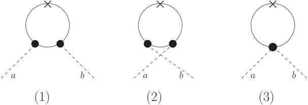
Figure 5: Diagrams of the effective chiral quark theory (A1) contributing to the matrix element $\langle\pi^{b}(p^{\prime})|\bar{\psi}^{f^{\prime}}(-\frac{\lambda n}{2})\,{\hbox to0.0pt{/\hss}n}\,\psi^{f}(\frac{\lambda n}{2})|\pi^{a}(p)\rangle$.

Then the result of Praszalowicz:2003pr for the integrals relevant for $-\xi\leq x\leq\xi$ reads:

$$\begin{split}&\mathcal{I}_{1}(x,\xi,t=0)=\frac{(-1)^{n+1}N_{C}M^{2}}{2(2\pi)^{2}F_{\pi}^{2}}\times\\ &\int_{0}^{\infty}d(\kappa_{\bot}^{2})\sum_{i=1}^{4n+1}\phi_{i}\frac{(x-1)^{6n+1}(f_{i}\,g_{i})^{n}}{{\prod_{k=1}^{4n+1}}B_{ik}D_{ik}}h_{1}^{(a)}(x,\xi),\end{split}$$ (B1)

where $N_{C}=3$ is the number of colors, $\kappa$ is the scaled variable ($\kappa^{\nu}=\frac{k^{\nu}}{\Lambda}$), $\mu=\frac{M}{\Lambda}$. For the definition of factors $f_{i}$, $g_{i}$, $B_{ik}$, $D_{ik}$ and $\phi_{i}$ see (B6), (B7).

$$\begin{split}&h_{1}^{(a)}(x,\xi)=\\ &\mu^{2}\left[(x-\xi)\frac{b_{i}^{2n}}{(x-\xi)^{2n}}+(x+\xi)z_{i}^{2n}-(x-1)\frac{d_{i}^{2n}}{(x+\xi)^{2n}}\right]+\\ &\frac{b_{i}^{2n}d_{i}^{2n}}{(x+\xi)^{4n}}z_{i}^{2n}\left[(\xi+1)\kappa_{\bot}^{2}+(\xi-x)(1+z_{i})\right].\end{split}$$ (B2)

For $-\xi\leq x\leq\xi$ $\mathcal{I}_{3}(x,\xi,t=0)$ reads:

$$\begin{split}&\mathcal{I}_{3}(x,\xi,t=0)=\\ &\frac{(-1)^{n+1}N_{C}M^{2}}{2(2\pi)^{2}F_{\pi}^{2}}\int_{0}^{\infty}d(\kappa_{\bot}^{2})\sum_{i=1}^{4n+1}\phi_{i}\left((x+\xi)z_{i}b_{i}\right)^{n}\times\\ &\frac{(x+\xi)^{2n+1}z_{i}^{2n}+(x-\xi)b_{i}^{n}}{\prod_{k=1}^{4n+1}B_{ik}}\,.\end{split}$$ (B3)

For $\xi\leq x\leq 1$ only the contribution of $\mathcal{I}_{1}$ is non-zero. It reads:

$$\begin{split}&\mathcal{I}_{1}(x,\xi,t=0)=\frac{(-1)^{n}N_{C}M^{2}}{2(2\pi)^{2}F_{\pi}^{2}}\times\\ &\int_{0}^{\infty}d(\kappa_{\bot}^{2})\sum_{i=1}^{4n+1}\phi_{i}\frac{(x-1)^{6n+1}(f_{i}\,g_{i})^{n}}{{\prod_{k=1}^{4n+1}}F_{ik}G_{ik}}h_{1}^{(b)}(x,\xi),\end{split}$$ (B4)

where

$$\begin{split}&h_{1}^{(b)}(x,\xi)=\\ &\mu^{2}\left[(x-\xi)\frac{g_{i}^{2n}}{(x-1)^{2n}}+(x+\xi)\frac{f_{i}^{2n}}{(x-1)^{2n}}-(x-1)z_{i}^{2n}\right]+\\ &\frac{f_{i}^{2n}g_{i}^{2n}}{(x-1)^{4n}}z_{i}^{2n}\left[\frac{\xi^{2}-1}{x-1}\kappa_{\bot}^{2}+\frac{\xi^{2}-x^{2}}{x-1}(1+z_{i})\right].\end{split}$$ (B5)

The symbols $b_{i}$, $d_{i}$, $B_{ik}$, $D_{ik}$ $f_{i}$, $g_{i}$, $F_{ik}$, $G_{ik}$ ($i,k=1,...,4n+1$) are defined as:

$$\begin{split}&b_{i}=2\xi(\kappa_{\bot}^{2}+1)+(\xi-X)z_{i}\,;\\ &d_{i}=-(1+\xi)(\kappa_{\bot}^{2}+1)+(x-1)z_{i}\,;\\ &B_{ik}=2\xi(\kappa_{\bot}^{2}+1)+(\xi-x)z_{i}+(\xi+x)z_{k}\,;\\ &D_{ik}=-(1+\xi)(\kappa_{\bot}^{2}+1)+(x-1)z_{i}-(\xi+x)z_{k}\,;\\ &f_{i}=-(1+\xi)(\kappa_{\bot}^{2}+1)-(\xi+x)z_{i}\,;\\ &g_{i}=(1-\xi)(\kappa_{\bot}^{2}+1)-(\xi-x)z_{i}\,;\\ &F_{ik}=-(1+\xi)(\kappa_{\bot}^{2}+1)-(\xi+x)z_{i}+(x-1)z_{k}\,;\\ &G_{ik}=(1-\xi)(\kappa_{\bot}^{2}+1)-(\xi-x)z_{i}-(x-1)z_{k}\,.\end{split}$$ (B6)

$z_{i}$, ($i=1,...,\,4n+1$) stand for the solutions of the master equation which controls the position of poles of the fermion propagator:

$$z^{4n+1}+z^{4n}-\frac{M^{2}}{\Lambda^{2}}=0\;.$$

The factors $\phi_{i}$ are introduced according to:

$$\phi_{i}=\prod_{k=1\atop k\neq i}^{4n+1}\frac{1}{z_{i}-z_{k}};\ \ \ \ \ \sum_{i=1}^{4n+1}z_{i}^{m}\phi_{i}=\begin{cases}0&\text{for}\;0\leq m<4n\\ 1&\text{for}\;m=4n\end{cases}\;.$$ (B7)

References

• (1) D. Müller, D. Robaschik, B. Geyer, F.M. Dittes, and J. Horejsi, Fortschr. Phys. 42, 101 (1994);
X. D. Ji, Phys. Rev. Lett.  78 (1997) 610 [arXiv:hep-ph/9603249];
A. V. Radyushkin, Phys. Lett.  B 380 (1996) 417 [arXiv:hep-ph/9604317];
X. D. Ji, Phys. Rev.  D 55 (1997) 7114 [arXiv:hep-ph/9609381];
J. C. Collins, L. Frankfurt and M. Strikman, Phys. Rev.  D 56 (1997) 2982 [arXiv:hep-ph/9611433].
• (2) K.Goeke, M.V.Polyakov, M.Vanderhaeghen, Progr. Part. Nucl. Phys. Vol.47, No 2, 401-515 (2001) [arXiv: hep-ph/0106012].
• (3) M. Diehl, Phys. Rept. 388, 41 (2003) [arXiv:hep-ph/0307382].
• (4) A.V. Belitsky and A.V. Radyushkin, Phys. Rept. 418, 1 (2005), [arXiv:hep-ph/0504030].
• (5) S. Boffi and B. Pasquini, “Generalized parton distributions and the structure of the nucleon,” arXiv:0711.2625 [hep-ph].
• (6) A. V. Radyushkin, Phys. Rev.  D 59, 014030 (1999) [arXiv:hep-ph/9805342].
• (7) M. V. Polyakov and C. Weiss, Phys. Rev.  D 60, 114017 (1999) [arXiv:hep-ph/9902451].
• (8) M. V. Polyakov, Nucl. Phys.  B 555, 231 (1999) [arXiv:hep-ph/9809483].
• (9) M. V. Polyakov and A. G. Shuvaev, “On ’dual’ parametrization of generalized parton distributions”, arXiv:hep-ph/0207153.
• (10) M. V. Polyakov, Phys. Lett.  B 659, 542 (2008) [arXiv:0707.2509 [hep-ph]].
• (11) M. V. Polyakov, “Educing GPDs from amplitudes of hard exclusive processes”, arXiv:0711.1820 [hep-ph].
• (12) M. V. Polyakov and M. Vanderhaeghen, “Taming Deeply Virtual Compton Scattering”, arXiv:0803.1271 [hep-ph].
• (13) A. M. Moiseeva and M. V. Polyakov, “Dual parameterization and Abel transform tomography for twist-3 DVCS”, arXiv:0803.1777 [hep-ph].
• (14) M. V. Polyakov, Phys. Lett.  B 555, 57 (2003) [arXiv:hep-ph/0210165].
• (15) I. V. Anikin and O. V. Teryaev, Phys. Rev.  D 76, 056007 (2007) [arXiv:0704.2185 [hep-ph]].
• (16) M. Diehl and D. Y. Ivanov, arXiv:0712.3533 [hep-ph].
• (17) D. Diakonov and V. Y. Petrov, Nucl. Phys.  B 272, 457 (1986).
• (18) V. Y. Petrov and P. V. Pobylitsa, arXiv:hep-ph/9712203.
• (19) V. Y. Petrov, M. V. Polyakov, R. Ruskov, C. Weiss and K. Goeke, Phys. Rev.  D 59, 114018 (1999) [arXiv:hep-ph/9807229].
• (20) M. V. Polyakov and C. Weiss, Phys. Rev.  D 59, 091502 (1999) [arXiv:hep-ph/9806390].
• (21) I. V. Anikin, A. E. Dorokhov, A. E. Maksimov, L. Tomio and V. Vento, Nucl. Phys.  A 678, 175 (2000).
• (22) I. V. Anikin, A. E. Dorokhov and L. Tomio, Phys. Part. Nucl.  31, 509 (2000) [Fiz. Elem. Chast. Atom. Yadra 31, 1023 (2000)].
• (23) M. Praszalowicz and A. Rostworowski, Phys. Rev.  D 66, 054002 (2002) [arXiv:hep-ph/0111196].
• (24) M. Praszalowicz and A. Rostworowski, Acta Phys. Polon.  B 34, 2699 (2003) [arXiv:hep-ph/0302269].