Local enrichment and its nonlocal consequences for victim-exploiter metapopulations
Abstract
The stabilizing effects of local enrichment are revisited. Diffusively coupled host-parasitoid and predator-prey metapopulations are shown to admit a stable fixed point, limit cycle or stable torus with a rich bifurcation structure. A linear toy model that yields many of the basic qualitative features of this system is presented. The further nonlinear complications are analyzed in the framework of the marginally stable Lotka-Volterra model, and the continuous time analog of the unstable, host-parasitoid Nicholson-Bailey model. The dependence of the results on the migration rate and level of spatial variations is examined, and the possibility of ”nonlocal” effect of enrichment, where local enrichment induces stable oscillations at a distance, is studied. A simple method for basic estimation of the relative importance of this effect in experimental systems is presented and exemplified.
pacs:
87.17.Aa,05.45.Yv,87.17.Ee,82.40.NpI Introduction
Spatially extended ecological systems, dispersal and metapopulation dynamics have attracted a lot of interest in recent years Kariva_Tilman1997 . In particular, the stability of an ecological system that contains many species interacting via competition, predation and symbiosis, and subject to environmental and demographic noise, poses an interesting mathematical and ecological puzzle. The role of dispersal among sites, migration amongst habitat patches, ”rescue” of a habitat by dispersal from other locations and so on, have been recognized as crucial ingredients in the stabilization mechanism.
This work concentrated on one of the basic ecological processes - the dynamics of victim-exploiter (predator-prey, host-parasitoid) populations. In the ”mean field” limit, i.e., where the chance for a predation event is fixed for any exploiter-victim pair, the simplest mathematical models are those of Lotka and Volterra Lotka1920 ; Volterra1931 for predator-prey, and Nicholson-Bailey Nicholson_Bailey1935 for host-parasitoid populations. Both models do not allow for an attractive manifold (such as fixed point, limit cycle or strange attractor). In fact, the coexistence point is either marginally stable (Lotka-Volterra like) or unstable (with the Nicholson-Bailey host parasitoid system as a prototype). In both cases one may expect to see extinction of (at least) one of the species after a short time; if the system is marginally stable the noise will drive it to extinction, while for an unstable manifold the system gravitates perpetually towards the edge of extinction.
How do victim-exploiter systems persist in nature for millions of years? One may suggest that the simple models are wrong, and assert that any realistic mathematical description of a victim-exploiter system should be ”dissipative”, supporting an attractive manifold. There are many modifications of the basic models that achieve these goals (e.g., by taking into account the finite carrying capacity of the environment or adding delayed response), and the observed population oscillations may be a result of noise perturbing an attractive fixed point McKane_Newman2005 . However, since the work of Gause Gause1934 through the classic experiments of Pimentel et al. Pimentel_ea1963 , Luckinbill Luckinbill1974 and Huffaker Huffaker1958 , it was known that small sized predator prey (or hosts and parasites) systems reach extinction in experimental time scales. The reason for this has become clear in the last decade, due to the experiments of Holyoak and Lawler Holyoak_Lawler1996 , Kerr et al. Kerr_ea2002 ; Kerr_ea2006 and Ellner et al. Ellner_ea2001 . In all of these experiments the same system goes extinct rapidly in the well-mixed limit while persisting way above the experimental time (up to h undreds of generations) when the population is spatially segregated. It follows that in many cases, and perhaps even generically, victim-exploiter systems are unstable in the well mixed limit, and acquire their stability due to its spatial structure.
What exactly stabilizes the spatial structure? a few answers have already been suggested. Some are related to the effect of spatial heterogeneity or spatio-temporal fluctuations, while others stress more generic mechanisms that may yield stability even if the space is perfectly homogenous. In this paper we focus on the effect of spatial heterogeneity (e.g., different growth rates on different spatial patches) as a stabilizer.
The observation that diffusive coupling between patches may stabilize otherwise unstable dynamics, or may result in convergence to a focus instead of a limit cycle, has been made in few disciplines independently. In ecology, Murdoch and Oaten Murdoch_Oaten1975 suggested that dispersal between Lotka-Voltera patches with spatial variability may stabilize the fixed point. Subsequent works by Crowley Crowley1981 , Ives Ives1992 , Murdoch et. al. Murdoch_ea1992 and Taylor Taylor1998 , extended this basic idea to include multi-patch systems, the effects of parasitoid aggregation, differences in diffusion parameters, density different migration and other complications that may occur in realistic systems. In chemistry, this stabilization is known alternatively as ”oscillator death” and was observed by Bar-Eli Bar-Eli1985 in the context of coupled chemical oscillators. That basic idea has since been applied to other diffusively coupled chemical systems, such as neural Kopel_Ermentrout1990 and calcium oscillations Tsaneva-Atanasova_ea2005 . Mathematically speaking, the stabilizing effect of diffusive coupling between two sites on a single species, extinction prone chaotic system has been considered by Gyllenberg et. al. Gyllenberg_ea1996 . These authors pointed out the ”salvage effect”, where the existence of a sink may stabilize the population on the source habitat; this effect also appears in the systems considered below.
Although the basic phenomenon is known, it turns out that the system of diffusively coupled unstable oscillations is quite rich and may reveal many interesting features beyond the stabilization of a fixed point. In this paper we analyze a very simple case of a single enriched site (where the prey, or host population flourish) surrounded by a less productive environment. We will examine in detail the conditions for the stability of the fixed point and the asymptotic behavior of the Lyapunov exponent, consider the possibility for the appearance of a limit cycle, and discuss the associated bifurcations. The most interesting phenomenon observed relates to the spatial population profile: here the effect of localized enrichment may yield either local or nonlocal changes, including the emergence of oscillations far from the location of enrichment, incommensurate oscillations, etc.
This paper is organized as follows: In the next section a linear toy model is presented and a few basic insights are derived. The effect of nonlinearities is emphasized for a predator-prey, marginally stable model in the third section. Although marginal stability is not a robust feature of a dynamical system and should not be considered seriously as the underlying dynamic of ecological processes, its consideration enables the attainment of basic knowledge regarding the effect of nonlinearity on stability, as will explained later on. The fourth section analyzes a Nicholson-Bailey like (unstable) system and discusses interesting nonlocal effects of enrichment. Finally, our results are discussed in view of the ”paradox of enrichment” Rosenzweig1971 , and possible experimental tests are suggested.
II A toy model: coupled linear oscillators
Let us present a linear model in order to exemplify some features of the fixed point stability (local analysis) for non-identical victim-exploiter patches. We consider two diffusively coupled harmonic oscillators (with the possibility of repulsive term with a positive constant ):
| (1) | |||||
As this system is linear, it may be diagonalized around the (only) fixed point at zero. When , the Lyapunov exponent for that fixed point turns out to be negative as long as for any , and approaches zero (marginal stability) if the dispersal is very small (no connection between oscillators), very large (single oscillator limit) or if the system is homogenous (). The Lyapunov exponent is given by:
| (2) |
and its typical behavior is illustrated in Figure 1. Linearity implies that if the fixed point is stable it is also globally attractive. The parametric dependence is characterized by the following properties:
-
•
Without loss of generality may be scaled to unity by rescaling of the time. Thus the stability is determined by three parameters: migration rate, repulsion () and the desynchronization term .
-
•
is a nonmonotonic function of the migration rate; close to zero migration, () vanishes linearly with , while for large diffusion it decays like . The optimal dispersal (given that other parameters hold fixed) is ; in which case .
-
•
The only effect of is a rigid upward shift of , as demonstrated in Figure 1, where the dashed line indicates the border between the stable and the unstable regime.
-
•
For fixed migration an increase of always helps to stabilize the system, but the effect saturates at . Accordingly, for any , there is a critical diffusion below which the system turns to be unstable, independent of the level of heterogeneity.
The limitations of this toy model are related to its linearity. In particular, once the fixed point at zero is unstable, the oscillation amplitude will grow unboundedly, and no other attractive manifold is allowed. This should not be the case if the coupled oscillators are nonlinear. One possible mechanism that may be responsible for an attractive manifold becomes clear if one looks at the system (II) in polar coordinates, where , (). In this representation the overall phase decouples and the phase space turns out to be three dimensional,
| (3) |
Where the phase desynchronization is , the amplitude desynchronization is , and the homogenous manifold is one dimensional . As implied from (II), the dynamic is either a flow towards an attractive fixed point at , or an unbounded growth of , depending on the relation between the stabilizing desynchronization factor and the repulsion . If the system is nonlinear, however, the angular velocity is generally dependent Abta_ea2007 . This implies that, although is too small close to zero, the ”effective ” may be larger far from the fixed point, leading to desynchronization and stabilization. In such a case one may expect a limit cycle in the nonlinear system. This, in fact, actually occurs, as will be demonstrated in the next sections.
Another limitation of the linear model is the fact that the location of the fixed point (at zero) is independent of the migration rate. Equations describing population dynamics support a nontrivial coexistence fixed point as well, and diffusion may alter not only its stability but also its location. In the next section we will show that the results for the asymptotic behavior of the Lyapunov exponent, as well as the saturation of for large , may not hold in more complicated nonlinear dynamics.
III Marginally stable Lotka-Volterra dynamics
Let us now take one step towards more realistic victim-exploiter systems, and consider the Lotka-Volterra continuous time dynamics, denoting the density of the predator population by , and the prey density by . On a single patch (say, when the population is well mixed, and the probability of encounter and predation is equal for any two individuals in the population) the pure LV system is marginally stable; there is a coexistence fixed point, but the system may also oscillate with any amplitude around this point, and the dynamic is determined by the initial conditions. Any type of stochasticity (demographic, environmental, random migration) will lead to random wandering of the system between all possible orbits. The amplitude of oscillations thus performs some sort of random walk, with the average amplitude growing in time until extinction Abta_ea2007 .
To consider the stabilizing effect of spatial differences in the environment, we will focus our attention on two typical situations: the case of two coupled patches, where the basic stability properties are to be demonstrated, and the case of a one dimensional ”chain” (with spatial patches and periodic boundary conditions) where the spatial population profile is examined.
We assume that predator-prey dynamics have the same parameters on all sites, the only exception is the ”zero” site where , the growth rate of the prey, is larger, i.e.,:
| (4) |
The corresponding Lotka-Volterra equations for a one dimensional array are:
| (5) |
where is the predator death rate, is the predation rate and and are the hopping rates of animals from one spatial patch to the other. Note that one can use the rescaling of the densities in order to take and set using the rescaling of time; this is the parametrization used hereon. Moreover, we focus here on the case of equal diffusivities .
As our system consists of one special site connected to a ”reservoir”, it turns out that the character of the reservoir is also of importance. A distinction should be made between the case of a single ”oasis” coupled to a desert, (i.e., where so the linear growth rate of both predator and prey is negative on all the patches except one) and the case where , where all sites are ”active”. Hereon, the first case will be regarded as an ”oasis-desert” situation (OD), where the case is named the poor-rich (PR) scenario.
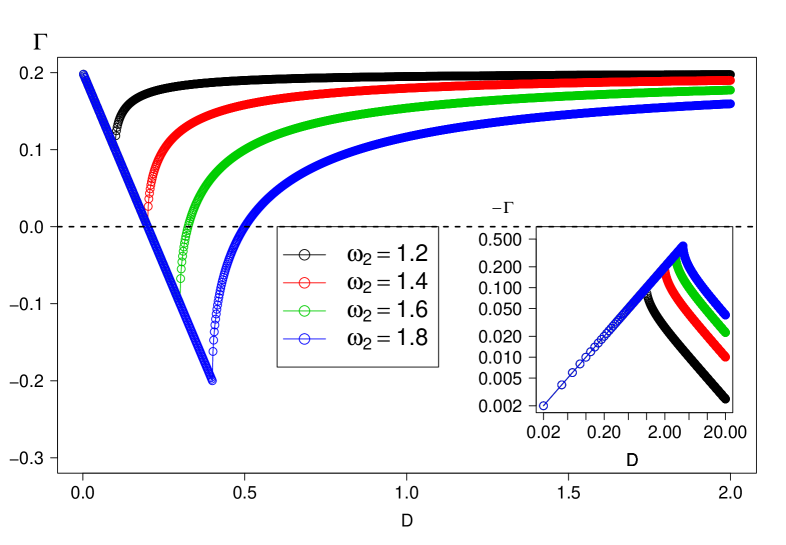
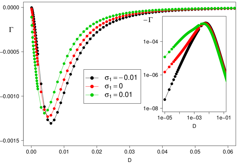
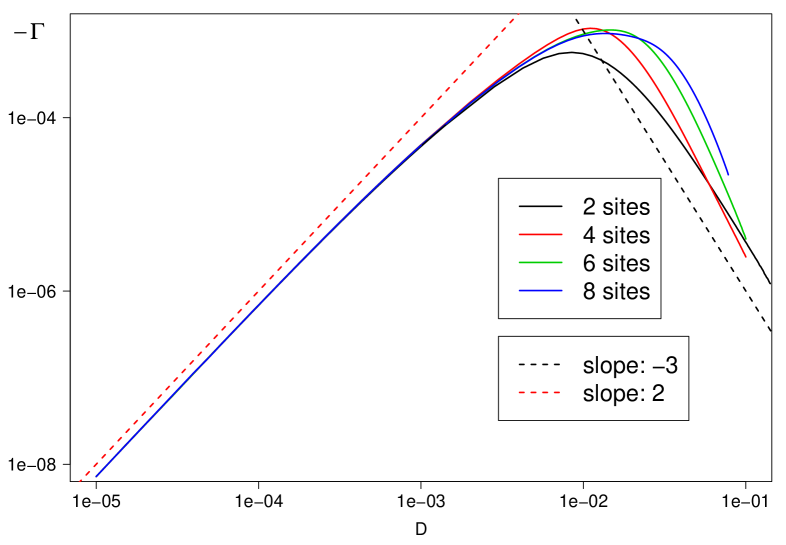
To begin, let us consider the two-patch case and examine the stability properties of the system. As the LV is marginally stable, one may expect that any spatial heterogeneity will yield stability. This is, indeed, the situation, as demonstrated in Figures 2. The general structure is very close to the linear model predictions with a few exceptions. First, the dependence of the Lyapunov exponent at small dispersal holds only in the PR case, while the OD scenario is characterized by asymptotic. Second, for the large asymptotic, approaches zero like instead of in the linear model. Both asymptotes may be obtained analytically as explained in appendix A. Note also the rightward migration of the optimal diffusion as the difference increases; this is the analog of the dependence of the linear model. As previously explained, the effects of nonlinearity have to do with the fact that the location of the fixed point itself depends on the migration rate. Beyond the two-patch limit, the stability properties are qualitatively the same, as demonstrated in Figure 3.
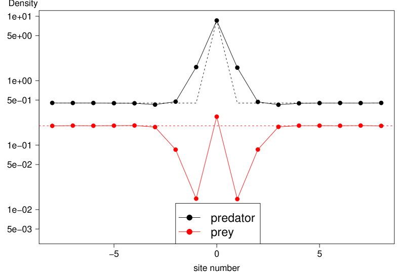
For the extended system one may consider not only the stability properties but also the spatial profile of the population densities. Let us consider first the oasis-desert scenario. Numerically solving the spatial configuration for (III) with the spatial heterogeneity defined by (4), one gets the colony profile presented in Figure 4. Clearly, deep in the desert the populations of both prey and predator are small, so the nonlinear (predation) terms in (III) are negligible. Accordingly, each of the species follows asymptotically the profile of a logistically growing population around an oasis Nelson_Shnerb1998 ; DNS ; Kariva_Tilman1997 , and the density decays like for the prey, and like for the predator. If we adopt the definition of the size of a colony as the length scale for which the population density is equal to some constant (this reflects the threshold introduced by the discreteness of the individuals), this size (up to logarithmic corrections) is for the prey and for the predator, where is the lattice spacing.
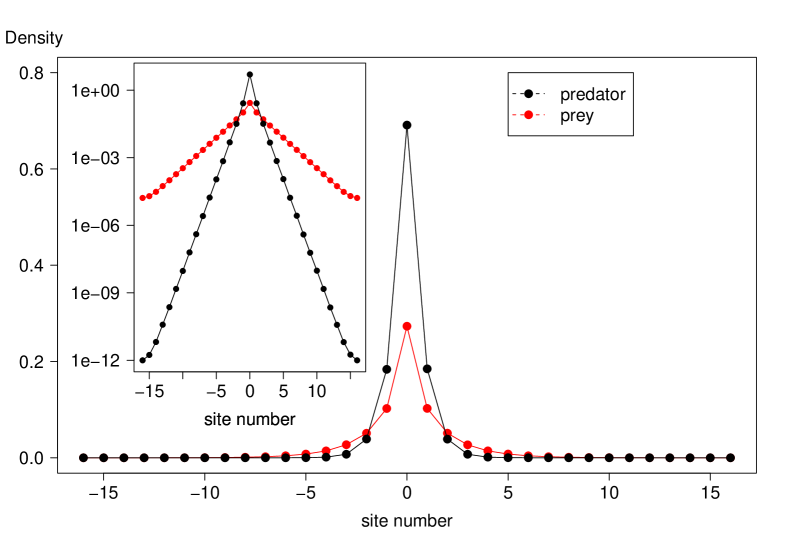
This result has two implications. First, in case of multiple oases, the interesting quantity is the typical distance between them in units of the colony size; if this is a large number, one should consider a system of two different patches, while a small number indicates strong mixing. The chance for a ”rescue effect” (where, due to noise, the population on one patch goes extinct until the ”rescue” by a rare immigrant from another habitat) may be very different for the victim and for the exploiter, depending on their death-diffusion ratio in the desert. Second, as demonstrated in Figure 4, the spatial decay of the colony may give false hints regarding the density at the oasis: in the example presented here, the predator population is rarely far away, but the predator abundance is much larger than that of the prey on the oasis. While the linear death rate of the prey is constant along the system and determines the exponential decay, its population on the oasis is dictated by the prey growth rate and is much higher.
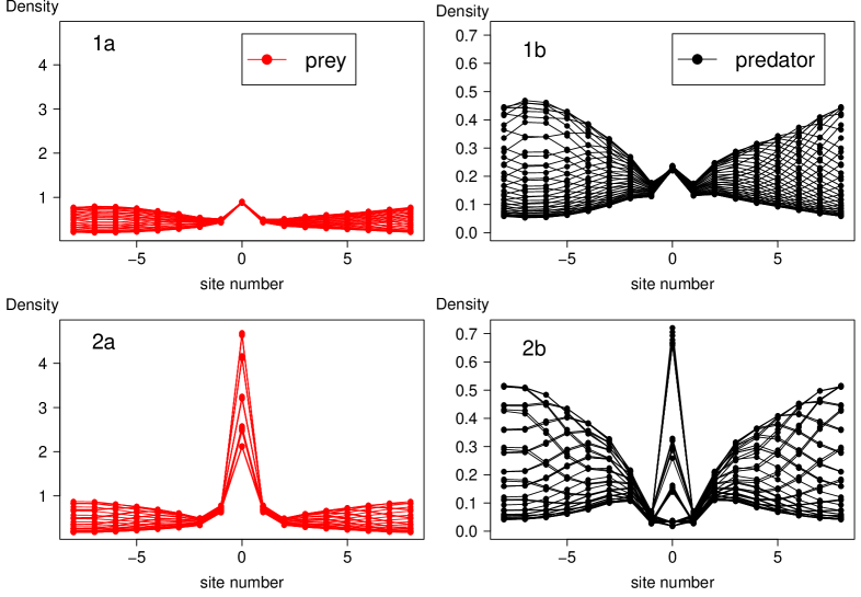
The effect of local enrichment becomes even more interesting in the poor-rich case, as one sees in Figure 5. An enrichment of the prey growth rate (say, by increasing the food supply) on a site leads to depletion of the prey in its neighborhood, while leaving the population on the rich site above its pre enrichment level. Surprisingly, the behavior of the prey density is paradoxical, but the ”paradox” is nonlocal.
IV Unstable systems: Nicholson-Bailey like model
The original mathematical description of a host-parasitoid system was formulated by Nicholson and Bailey Nicholson_Bailey1935 . If the host density is given by and the parasitoid is , Nicholson and Bailey map for nonoverlapping generations is:
| (6) |
where is the fecundity of the host in the absence of the parasitoid, is the infectivity (the chance of a single parasitoid to infect the host) and is the number of parasites produced by a single infection.
The essential feature of the NB model is its instability - it allows ever growing oscillations around its coexistence fixed point. However, the model does not allow explicitly for extinction, as P and H are positive definite along the process. As the oscillations grow, the minimal distance from the extinction phase for each of the species decays rapidly. Hence, for any realistic system, where small noise or the discreteness of individuals are taken into account, the system flows deterministically to the extinction phase.
One technical characteristic of the NB dynamics makes its analysis problematic in the context of the current discussion. Eqs. (IV) assume nonoverlapping generations, and the corresponding map, when extended to diffusively coupled spatial domains, supports attractive periodic orbits with finite basin of attraction adler . Even in the absence of spatial inhomogeneities some initial conditions are trapped in the periodic orbits, and it is hard to distinguish between this effect and stabilization due to spatial differences. In order to focus the discussion on the consequences of local enrichment, we will switch here to continuous time dynamics that imitates the relevant features of the NB model. For the sake of nonlinear dynamics analysis considered here, our model is equivalent to the small limit of the NB system, where the map may be approximated by continuous time equations, as emphasized in figure 6.
Let us assume, thus, that in a predator-prey system the encounter between a single predator and prey may result in predation, but the predation probability increases if two predators encounter a single prey (i.e., there is a predation ”Allee effect”). We ”enrich” the LV system with additional terms that correspond to this ally predation process:
| (7) |
The resulting equations admit a coexistence fixed point at , , where . This fixed point is unstable, with a positive local Lyapunov exponent. The amplitude of oscillation increases rapidly with time, but the system cannot reach the extinction phase unless some noise is presented.

To include spatial structure, we switch to a nondimensionalized form of the diffusively coupled patch system, where the definition of constants is identical with Eq. III:
| (8) |
Again, one should expect to recover the zero dimensional dynamics as approaches zero and infinity. In between, the resulting dynamics turn out to be quite rich. As in the LV case, we will check the two-patch system to get the general picture for the stability of the system, then look at a multi-patch example to see the spatial profile.
The linear model admits two options: in the presence of spacial variation the unstable system may remain unstable (in which case it flows to extinction exponentially fast) or admit (for intermediate diffusivities) an attractive fixed point. As exemplified in Figure 7, the nonlinear model (IV) turns out to admit another option: while the fixed point may be unstable, the system does not flow to extinction but to an attractive manifold like a limit cycle. This gives rise to many complications in the system behavior, including various types of bifurcations, bistability and hysteresis. Partial analysis of the bifurcations and the phase portraits for the unstable case is presented in Appendix B.
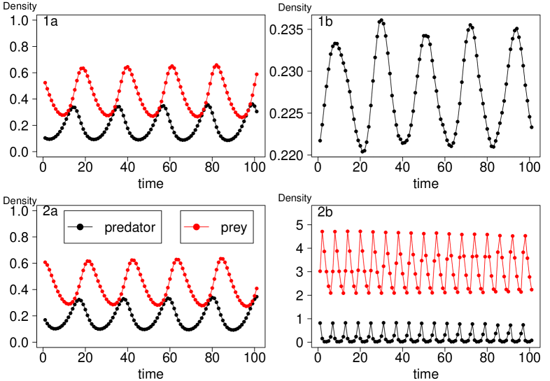
As in the marginally stable LV case, one observes a nonlocal effect of enrichment on the spatial profile. In Figure 8 a few possibilities are demonstrated. It may happen that nutrient enrichment at a single site causes the other parts of the system to change periodically, while the rich site population is almost fixed. Increasing the spatial variation, the amplitude of oscillations on the rich site grow (Figure 9), and at the same time the phase locking with the ”wings” is lost. At the end, the oscillations at the center and on the wings become incommensurate, giving rise to an attractive torus, as demonstrated in Figure 10. In the oasis-desert case the effect is less dramatic, and the oscillations appear first in the enriched region (Figure 11).

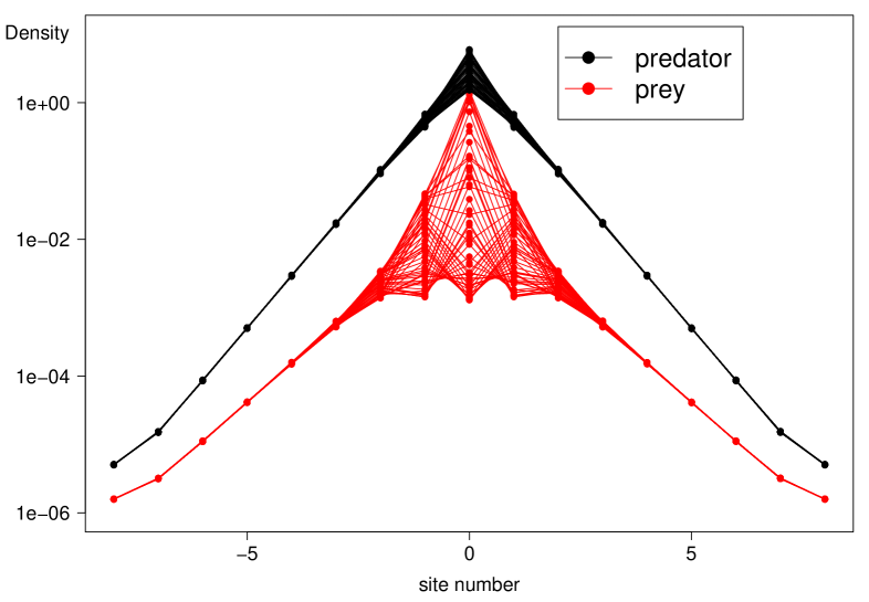
V Discussion
The effect of quenched spatial variations, where the habitat is made of local patches connected by dispersal, is stabilizing. Besides the survey of the possible states of this dynamical system and the asymptotical behavior for large and small migration rates, the nonlocal effect of enrichment emerges from the numerics as a new feature. In particular, it turns out that local enrichment may stabilize otherwise unstable system, and that the limit cycle may involve periods of large amplitude far from the enriched site, while the rich site itself involves cycles of negligible amplitude. Increasing the spatial heterogeneity, one observes an increase in oscillation amplitude on the rich site, while its neighborhood remains relatively calm. The oscillations at the enriched site may be incommensurate with the period of oscillations at the ”wings”, such that the system flows into a stable torus instead of a limit cycle.
This observation may solve the ”paradox of enrichment” Rosenzweig1971 in some cases. Many victim-exploiter models predict an increase in oscillation amplitude as a result of increased prey growth rate or carrying capacity. The empirical support of this prediction, however, is quite limited Tilman_Wedin1991 and in many experiments the effect is absent Murdoch_McCauley1985 ; Kirk1998 . From the results here one concludes that in some cases, small spatial fluctuations in the enrichment, e.g., small inhomogeneities in the concentration of food, sunlight or other resources, may stabilize the system and avoid the ”paradoxical” behavior.
What degree of enrichment uniformity is required in order to observe the paradoxical behavior? Such a question may be analyzed very easily using the toy model presented here as a basic tool for parameter estimation. As stressed above, only three parameters control the system close to the fixed point: the dispersal rate , the repulsion and the desynchronization factor . The threshold between a ”uniform like” and heterogenous system appears at , i.e., when the migration rate in/out of a patch (here a patch is defined as a region where the resource distribution is uniform) is close to the desynchronazation rate, given by the difference in oscillation period between patches. If diffusion is much larger, the system should be considered as uniform. Much smaller diffusion corresponds to the situation of almost independent patches.
For an experimental system, one should try to gain a rough estimate of the above parameters in order to ascertain the level of enrichment needed to yield a strong enough effect. Here we exemplify these considerations using two experiments: one on a predator-prey system and the other host-parasitoid.
In the experiment of Kerr et al Kerr_ea2006 , E-coli bacteria is the host and its viral pathogen, T4 coliphage, is the parasite. In the well-mixed case, the system survives about 24h before the bacteria undergoes extinction; this corresponds to seconds. The migration in that experiment is controlled by the experimentalists, as a robot taking biological material between otherwise disconnected patches. The authors present simulations, based on empirically calibrated cellular automata, that predict oscillations with a time scale of about 10 days, so is about , i.e., close to . If one chooses a day as the unit time, . From the linear system analysis, it seems that this system should be coupled to another one with in order to observe stabilization due to spatial heterogeneity.
Another example is the experiment of Holyoak and Lawler Holyoak_Lawler1996 , where the predaceous ciliate Didinium nasutom is feeding on the bacterivorous ciliate Colpidium cf. Striatum. The diffusion constant for these small (length of order 0.1-0.05 mm) creatures depends on the level of water turbulence and on the size of the tubes connecting different microcosms. The extinction time in the well mixed case is about 70 days ( seconds) and is about 10 days. In the appropriate dispersal, one may observe stabilization if the system is coupled to another set of microcosms with , i.e., relatively small enrichment will allow for stabilization.
We acknowledge helpful discussions with Marcel Holyoak. This work was supported by the EU 6th framework CO3 pathfinder and DAPHNet.
VI Appendix A
In this appendix we discuss the dependence of the system’s stability (its Lyapunov exponent) on the rate of animal dispersal. As explained above, one should recover the mean field results in the case of no migration, , and as the migration rate approaches infinity. For the Lotka-Voltera, marginally stable case, the Lyapunov exponent vanishes in these two limits, while in between it is finite and negative. We now want to explore the two limits more carefully and attain the asymptotic dependence of the Lyapunov exponent in terms of the system parameters.
To begin, let us consider the simplest spatially explicit case, i.e., a two-patch LV system. The dynamics in such a case are four dimensional and described by:
| (9) |
where the growth parameter is heterogenous. Clearly, as approaches infinity the differences between patches, and approach zero, so it is useful to rotate the coordinate system in order to separate between the homogenous manifold ( and ) and the manifold. Defining, now, , and assuming that (and the same for B) while (and the same for ), one can solve for the fixed point of the set of equations (VI), order by order in up to, say, order . This solution is then plugged into the stability matrix, and the roots of the characteristic polynomial may then be found (again, order by order in ) up to . With that, one finds that the leading contribution to the Lyapunov exponent (the first order for which the root of the characteristic polynomial admits a real part) is . The asymptotics of the Lyapunov exponent for large D turns out to be:
| (10) |
Close to , on the other hand, one should use another technique. Solving and to the n-th order in , these have to be plugged into the stability matrix, from which the characteristic polynomial is extracted. For , two (in the oasis-desert case) or all four (in the poor-rich case) of the eigenvalues are purely imaginary. The corrections to these imaginary eigenvalues are written as a power series in , and one finds that the real part of the slowly decaying eigenfunction (i.e., the Lyapunov exponent) is in the poor-rich case, but only for the oasis-desert situation. For (oasis desert situation) one gets:
| (11) |
While in the poor-rich case for the exponent is:
| (12) |
This result does not hold when the system approaches the uniform limit , as it has been obtained perturbatively, neglecting the degeneracy appearing for these parameters.
VII Appendix B
In this appendix we consider the various equilibrium states of the unstable dynamics (IV) on a heterogenous environment (IV). The 4d system is quite complicated and allows for many types of bifurcations. In the following, a general sketch of the main types of dynamical behavior is given.
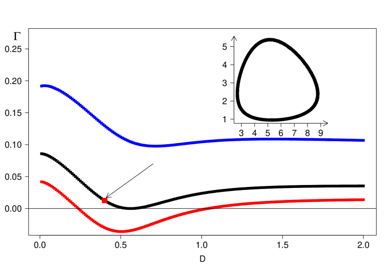
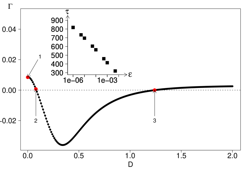
Let us take a look at Figure 12, which describes the Lyapunov exponent of the coexistence fixed point vs. . In the region of intermediate migration (between 2 and 3), the coexistence point becomes attractive due to the heterogeneity, similar to the LV system. However, at 2 the system undergoes a supercritical Hopf bifurcation, and a globally attractive limit cycle appears. As the diffusion constant approaches zero the radius of this limit cycle diverges, and finally it losses its stability via homoclinic bifurcation, and the cycle period diverges logarithmically as shown in the inset to Figure 12.
There exists, however, another set of parameters, where the coexistence fixed point does not acquire stability for any diffusion rate, as demonstrated in Figure 13. It turns out that, in this case, the limit cycle born via homoclinic bifurcation at loses its stability through an infinite period bifurcation at larger dispersal values, leaving an unstable system with oscillations that grow unboundedly until extinction. The stable cycle reemerges at even higher values of , while now its size grows as diffusion increases. It should be noted that in some cases (like the parameter range that corresponds to the middle curve in Figure 7) we have observed a limit cycle behavior for any value of .

References
- [1] P. Kariva and D. Tilman. Princeton University Press, Princeton NJ, 1997.
- [2] A. J. Lotka. Analytical note on certain rhythmic relations in organic systems. Proc. Natl. Acad. Sci. USA, 6:410–415, 1920.
- [3] V. Volterra. Variations and Fluctuations of the Number of individuals in animal Species living together. Mc Graw Hill, NY, 1931.
- [4] A.J. Nicholson and V.A. Bailey. The balance of animal populations. Proc. Zool. Soc. London, 3 Part I:551–598, 1935.
- [5] A. J. McKane and T. J. Newman. Predator-prey cycles from resonant amplification of demographic stochasticity. Phys. Rev. Lett., 94:218102, 2005.
- [6] G.F. Gause. William and Wilkins, Baltimore, 1934.
- [7] D. Pimentel, Nagel W.P., and J.L. Madden. Space-time structure of the environment and the survival of parasite-host systems. Am. Nat., 97:141–167, 1963.
- [8] L.S. Luckinbill. The effects of space and enrichment on a predator-prey system. Ecology, 55(5):1142–1147, 1974.
- [9] C.B. Huffaker. Experimental studies on predation: dispersion factors and predator prey oscillations. Hilgardia, 27:343–383, 1958.
- [10] M. Holyoak and S. P. Lawler. Persistence of an extinction-prone predator-prey interaction through metapopulation dynamics. Ecology, 77:1867–1879, 1996.
- [11] B. Kerr, M.A. Riley, M.W. Feldman, and B.J.M. Bohannan. Local dispersal promotes biodiversity in a real-life game of rock-paper-scissors. Nature, 418:171–174, 2002.
- [12] B. Kerr, C. Neuhauser, B.J.M. Bohannan, and A.M. Dean. Local migration promotes competitive restraint in a host-pathogen ’tragedy of the commons’. Nature, 442:75–78, 2006.
- [13] S.P. Ellner, E. McCauley B. E. Kendall, C. J. Briggs, P. R. Hosseini, S. N. Wood, A. Janssen, M. W. Sabelis, P. Turchin, R. M. Nisbet, and W. W. Murdoch. Habitat structure and population persistence in an experimental community. Nature, 412:538–543, 2001.
- [14] W. W. Murdoch and A. Oaten. Predation and population stability. Adv. Ecol. Res., 9:1–131, 1975.
- [15] P. H. Crowley. Dispersal and the stability of predator-prey interactions. Am. Nat., 118:673–701, 1981.
- [16] A.R. Ives. Continuous-time models of host-parasitoid interactions. Am. Nat., 140:1–29, 1992.
- [17] W. W. Murdoch, C.J. Briggs, R.M. Nisbet, W.S.C. Gurney, and A. Stewart-Oaten. Aggregation and stability in metapopulation models. Am. Nat., 140:41–58, 1992.
- [18] A.D. Taylor. Environmental variability and the persistence of parasitoid-host metapopulation models. Theo. Pop. Biol., 53:98–107, 1998.
- [19] K. Bar-Eli. On the stability of coupled chemical oscillators. Physica D, 14:242–252, 1985.
- [20] N. Kopel and Ermentrout G.B. Oscillator death in systems of coupled neural oscillators. SIAM J. Appl. Math., 50(1):125–146, 1990.
- [21] K. Tsaneva-Atanasova, D.I. Yula, and Sneyd J. Calcium oscillations in a triplet of pancreatic acinar cells. Biophysical Journal, 88:1535–1551, 2005.
- [22] M. Gyllenberg, A.V. Osipov, and G. Soderbacka. Bifurcation analysis of a metapopulation model with sources and sinks. Journal of nonlinear science, 6:329 – 366, 1996.
- [23] M.L. Rosenzweig. Paradox of enrichment: Destabilization of exploitation ecosystems in ecological time. Science, 171:385, 1971.
- [24] R. Abta, M. Schiffer, and N. M. Shnerb. Amplitude dependent frequency, desynchronization, and stabilization in noisy metapopulation dynamics. Phys. Rev. Lett., 98:098104, 2007.
- [25] David R. Nelson and Nadav M. Shnerb. Non-hermitian localization and population biology. Phys. Rev. E., 58(2):1383–1403, Aug 1998.
- [26] David R. Nelson Karin Dahmen and Nadav M. Shnerb. Life and death near a windy oasis.
- [27] F.R. Adler. Migration alone can produce persistence of host parasitoid models. Am. Nat., 141:642, 1993.
- [28] D. Tilman and D. Wedin. Oscillations and chaos in the dynamics of a perennial grass. Nature, 353:653–655, 1991.
- [29] W. W. Murdoch and E. McCauley. Three distinct types of dynamic behaviour shown by a single planktonic system. Nature, 316:628–630, 1985.
- [30] K.L. Kirk. Enrichment can stabilize population dynamics: Autotoxins and density dependence. Ecology, 79(7):2456–2462, 1998.