Double-exciton component of the cyclotron spin-flip mode in a quantum Hall ferromagnet

Abstract

We report on the calculation of the cyclotron spin-flip excitation (CSFE) in a spin-polarized quantum Hall system at unit filling. This mode has a double-exciton component which contributes to the CSFE correlation energy but can not be found by means of a mean field (MF) approach. The result is compared with available experimental data.

PACS numbers 73.21.Fg, 73.43.Lp, 78.67.De

A two-dimensional electron gas (2DEG) in a high perpendicular magnetic field possesses many remarkable features.an82 In particular, it presents a rare case of strongly correlated system governed by real Coulomb interaction (not by a model Hamiltonian!) where, nevertheless, some solutions of the quantum many-body problem can be found exactly. Indeed, under the conditions of integer quantum Hall effect (when the filling factor is $\nu=1,2,3,...$), the one-cyclotron magnetoplasma and the lowest spin-flip modes are calculated analytically to the leading order in the parameter $r_{\rm c}\!=\!E_{\rm C}/\hbar\omega_{c}$. by81 ; by83 ; ka84 ; di05 [$\omega_{c}$ is the cyclotron frequency; $E_{\rm C}\!=\alpha e^{2}/\kappa l_{B}$ is the characteristic interaction energy, $\alpha$ being the average form-factor related to the finite thickness of the 2DEG ($0.3\,\raise 1.72218pt\hbox{$<$}\kern-8.00003pt\lower 3.01385pt\hbox{$\sim$}\,\alpha\!<\!1$); $l_{B}$ is the magnetic length.] This astounding property is the feature of either filled or half-filled highest-occupied Landau level (LL) where the simplest-type excitations are single excitons or superposition of single-exciton modes. The many-body problem is thereby reduced to the two-body one, i.e. to the interaction of electron with an effective hole. Being quite in the context of similar studies, the present letter concerns however the case which can not be reduced to a single-exciton problem.

We remind that 2DEG excitons are characterized by sublevels $a\!=\!(n_{a},\sigma_{a})$ and $b\!=\!(n_{b},\sigma_{b})$ where electron is promoted from the $n_{a}$-th LL with spin-component $S_{z}\!=\!\sigma_{a}$ to the $n_{b}$-th LL with $S_{z}\!=\!\sigma_{b}$. The relevant quantum numbers are $\delta n\!=\!n_{b}\!-\!n_{a}$, $\delta S_{z}\!=\!\sigma_{b}\!-\!\sigma_{a}$, and the two-dimensional (2D) wave vector ${\bf q}$. The single exciton problem is exactly solvable in the following cases: (i) at odd filling $\nu$ when $\delta n\!=\!1$ and $\delta S_{z}\!=\!0$ (magnetoplasmon) or $\delta n\!=\!0$ and $\delta S_{z}\!=\!-1$ (spin wave);by81 ; ka84 ; dizh05 (ii) at even $\nu$ when $\delta n\!=\!1$ and $\delta S_{z}\!=\!0,\pm 1$ (magnetoplasmon and spin-flip triplet).ka84 ; di05 ; dizh05 At the same time the two-body problem may be discussed within a MF approach (in some publications called ‘time-dependent Hartree-Fock’ approximation mc85 ; lo93 ) which excludes any quantum fluctuations from a single exciton to double- or many-exciton states. For the above simplest cases of $\delta n$ and $\delta S_{z}$, the MF calculation gives an asymptotically exact result which may be found perturbatively to the first order in $r_{\rm c}$,foot1 because these $(\delta n,\,\delta S_{z})$ sets can not correspond to any states except single-exciton modes. Any complication of $(\delta n,\delta S_{z})$ makes the calculations substantially more difficult due to the necessary expansion of the basis to the entire continuous set of many-exciton states with the same total numbers $\delta n$, $\delta S_{z}$, and ${\bf q}$. For example, the double-cyclotron plasmon with $\delta n\!=\!2$, $\delta S_{z}\!=\!0$ and with given ${\bf q}$ ‘dissociates’ into double-exciton states consisting of one-cyclotron plasmon’s pairs with the total momentum equal to ${\bf q}$.ka84 At odd $\nu$, a similar ‘dissociation’ occurs for the CSFE, where $\delta n\!=\!-\delta S_{z}\!=\!1$. The proper double-exciton states are pairs of a magnetoplasmon ($\delta n\!=\!1,\,\delta S_{z}\!=\!0$) and a spin wave ($\delta n\!=\!0,\,\delta S_{z}\!=\!-1$). The problem thus changes from the two-body case to the four-body one, and the correct solution should be presented in the form of combination of the single-exciton mode and continuous set of double-exciton states.dizh05 It is important that in both cases the desired solution corresponds to a discrete line against the background of a continuous spectrum of free exciton pairs. The technique of correct solution has to be of essentially non-Hartree-Fock (non-HF) type. Actually this letter concerns the fundamental question of consistency of the MF approach.

By considering the case of unit filling factor where the number of electrons is equal to the number of magnetic flux quanta $N_{\phi}$, now we report on a study of the CSFE with ${\bf q}\!=\!0$. This state is optically active and identified in the ILS experiments.pi92 ; va06 Besides, it is exactly this spin-flip magnetoplasma mode which is the key component of the elementary perturbation used in the microscopic approach to the skyrmionic problem.di02 The calculation is performed in ‘quasi-analytical’ way which should, in principle, lead to the result which is exact in the leading approximation in $r_{\rm c}$. In our case the envelope function determining the combination of the double-exciton states is one-dimensional — i.e., it only depends on the modulus of the excitons’ relative momentum. This function is chosen in the form of expansion over infinite orthogonal basis, where every basis vector obeys a specific symmetry condition necessary for the total envelope function. Even to the first-order approximation in $r_{\rm c}$, we obtain a non-HF correction to the former HF result pi92 ; lo93 for the CSFE energy.

As a technique, we use the excitonic representation (ER) which is a convenient tool for description of the 2DEG in a perpendicular magnetic field.dz83 ; di05 ; dizh05 When acting on the vacuum $|{\rm 0}\rangle$ (in our case $|{\rm 0}\rangle\!=\!|\overbrace{\uparrow,\uparrow,...\uparrow}^{\displaystyle{\vspace{-5mm}\mbox{\tiny{$\;N_{\phi}$}}^{\vphantom{\int^{\infty}}}}}\,\rangle$), the exciton operators produce a set of basis states which diagonalize the single-particle term of the Hamiltonian and some part ${\hat{H}}_{\rm ED}$ of the interaction Hamiltonian.dizh05 ; di02 Exciton states are classified by ${\bf q}$, and it is essential that in this basis the LL degeneracy is lifted.

So, the generic Hamiltonian is ${\hat{H}}\!=\!{\hat{H}}_{1}\!+\!{\hat{H}}_{\rm int}$ where

$$\begin{array}[]{l}{\hat{H}}_{1}=\sum\limits_{\sigma}\int\!d{\bf r}\,{\hat{\Psi}}_{\sigma}^{\dagger}({\bf r})\left[\frac{1}{2m^{*}}\left(i{\vec{\nabla}}-{e\vec{A}/c}\right)^{2}\!+\!g\mu_{B}B{\hat{S}}_{z}\right]\!{\hat{\Psi}}_{\sigma}({\bf r})\quad\mbox{and}\\ {\hat{H}}_{\rm int}=\frac{1}{2}\sum\limits_{\sigma_{1},\sigma_{2}}\int\!d{\bf r}_{1}d{\bf r}_{2}\,{\hat{\Psi}}_{\sigma_{2}}^{\dagger}({\bf r}_{2}){\hat{\Psi}}_{\sigma_{1}}^{\dagger}({\bf r}_{1})U({\bf r}_{1}\!-\!{\bf r}_{2}){\hat{\Psi}}_{\sigma_{1}}({\bf r}_{1}){\hat{\Psi}}_{\sigma_{2}}({\bf r}_{2}).\end{array}$$

Choosing, e.g, the Landau gauge and substituting for the Schrödinger operator ${\hat{\Psi}}^{\dagger}_{\sigma}\!\!=\!\!\sum_{np}a^{\dagger}_{np\sigma}\psi_{np\sigma}^{*}$ (indexes $n,p,\sigma$ label the LL number, intra-LL state, and spin sublevel), one can express the Hamiltonian (1) in terms of combinations of various components of the density-matrix operators.di05 ; dizh05 ; di02 These are exciton operators defined as dz83 ; di05 ; dizh05 ; di02

$${{\cal Q}}_{ab{\bf q}}^{{\dagger}}={N_{\phi}}^{-1/2}\sum_{p}\,e^{-iq_{x}p}b_{p+\frac{q_{y}}{2}}^{{\dagger}}\,a_{p-\frac{q_{y}}{2}}\quad\mbox{and}\quad{{\cal Q}}_{ab{\bf q}}={{\cal Q}}_{ba\,-{\bf q}}^{{\dagger}}$$

and obeying the commutation algebra dizh05

$$\left[{\cal Q}_{cd\,{\bf q}_{1}}^{{\dagger}},{\cal Q}_{ab\,{\bf q}_{2}}^{{\dagger}}\right]\!\equiv\!N_{\phi}^{-1/2}\left(e^{-i({\bf q}_{1}\!\times{\bf q}_{2})_{z}/2}\delta_{b,c}{\cal Q}_{ad\,{\bf q}_{1}\!+\!{\bf q}_{2}}^{{\dagger}}-e^{i({\bf q}_{1}\!\times{\bf q}_{2})_{z}/2}\delta_{a,d}{\cal Q}_{cb\,{\bf q}_{1}\!+\!{\bf q}_{2}}^{{\dagger}}\right)$$

(in our units $l_{B}\!=\!\sqrt{c\hbar/eB}\!=\!1$). Here $a,b,c,...$ are binary indexes (see above), which means that $a_{p}^{\dagger}\!=\!a_{n_{a}p\,\sigma_{a}}^{\dagger}$, $b_{p}^{\dagger}\!=\!{a}^{\dagger}_{n_{b}p\,\sigma_{b}}$… We will also employ for binary indexes the notations $n\!=\!(n,\uparrow)$ and ${\overline{n}}\!=\!(n,\downarrow)$, so that the single-mode component of the CSFE is defined as ${\cal Q}^{\dagger}_{0\overline{1}{\bf q}}|0\rangle$. The interaction Hamiltonian can be presented as ${\hat{H}}_{\rm int}\!=\!{\hat{H}}_{\rm ED}\!+{\hat{H}}^{\prime}$ where ${\hat{H}}_{\rm ED}$, if applied to the state ${{\cal Q}}_{ab{\bf q}}^{{\dagger}}|0\rangle$, yields a combination of single-exciton states with the same numbers $\delta n$, $\delta S_{z}$, and ${\bf q}$ (see Refs. dizh05, ; di02, and therein ${\hat{H}}_{\rm ED}$ expressed in terms of exciton operators). In the framework of the above HF approximation, the CSFE correlation energy pi92 ; lo93 is obtained from the equation ${\cal E}_{0\overline{1}}({q})\!=\!\langle{\mbox{\rule{0.0pt}{11.38109pt}}}0|{\cal Q}_{0\overline{1}{\bf q}}[{\hat{H}}_{\rm int},{\cal Q}_{0\overline{1}{\bf q}}^{{\dagger}}]|0{\mbox{\rule{0.0pt}{11.38109pt}}}\rangle$ where only the ${\hat{H}}_{\rm ED}$ part of the interaction Hamiltonian contributes to the expectation. In the following, we need this so-called HF value at $q=0$, namely ${\cal E}_{0\overline{1}}(0)\!\equiv\!{\cal E}_{\rm HF}\!=\!\frac{1}{2}\int_{0}^{\infty}{p^{3}dp}V(p)e^{-p^{2}/2}$ where $2\pi V(q)$ is the Fourier component of the effective Coulomb vertex in the layer.pi92 (In the strictly 2D limit $\alpha\!\to\!1$, and $V(q)\!\to e^{2}/\kappa l_{B}q$.)

The problem arises due to the ‘troublesome’ part ${\hat{H}}^{\prime}$ of the interaction Hamiltonian which can not be diagonalized in terms of single-exciton states. For our task we keep in ${\hat{H}}^{\prime}$ only the terms contributing to $\left[{\hat{H}}^{\prime},{\cal Q}_{0\overline{1}{\bf q}}^{{\dagger}}\right]|0\rangle$ and besides preserving the cyclotron part of the total energy (i.e. commuting with ${\hat{H}}_{1}$). In terms of the ER these are  di05 ; dizh05

$${\hat{H}}_{0{\overline{1}}}^{\prime}=\sum_{\bf q}\frac{q^{2}}{2}V(q)e^{-q^{2}/2}{{\cal Q}}_{01{\bf q}}^{{\dagger}}{{\cal Q}}_{\overline{0}\,\overline{1}{\bf q}}\;+\;\mbox{H.c.}$$

Using Eqs. (3) and identities ${\cal Q}^{\dagger}_{aa{\bf q}}|0\rangle\!\equiv\!N_{\phi}^{-1/2}\delta_{{\bf q},{\bf 0}}|0\rangle$ if $a\!=\!(0,\uparrow)$ and ${\cal Q}^{\dagger}_{aa{\bf q}}|0\rangle\!\equiv\!0$ if $a\!\not=\!(0,\uparrow)$, one can find that the operation of ${\hat{H}}_{0{\overline{1}}}^{\prime}$ on vector ${\cal Q}_{0\overline{1}{\bf q}}^{{\dagger}}|0\rangle$ results in a combination of states of the type of ${N_{\phi}}^{-1/2}\sum_{\bf s}f({\bf s}){\cal Q}_{0\overline{0}\,{\bf q}/2\!-\!{\bf s}}^{\dagger}{\cal Q}_{01\,{\bf q}/2\!+\!{\bf s}}^{\dagger}|0\rangle$ with a certain regular and square integrable envelope function, $\int\!|f({\bf s})|^{2}d{\bf s}\!\sim\!1$. The norm of this combination is not small as compared to $\langle 0|{\cal Q}_{0\overline{1}{\bf q}}{\cal Q}^{\dagger}_{0\overline{1}{\bf q}}|0\rangle\!\equiv\!1$, and the terms (4) must be taken into account when calculating the CSFE energy.

On the other hand, if the set of double-exciton states $|{\bf s},{\bf q}\rangle\!=\!{\cal Q}_{0\overline{0}\,{\bf q}/2\!-\!{\bf s}}^{{\dagger}}{\cal Q}_{01\,{\bf q}/2\!+\!{\bf s}}^{{\dagger}}|0\rangle$ is considered, then one finds that they, first, are not exactly but ‘almost’ orthogonal: $\langle{\bf q}_{1},{\bf s}_{1}|{\bf s}_{2},{\bf q}_{2}\rangle\!=\!\delta_{{\bf q}_{1},{\bf q}_{2}}\left\{\delta_{{\bf s}_{1},{\bf s}_{2}}\right\}$, where $\left\{\delta_{{\bf s}_{1},{\bf s}_{2}}\right\}\!\equiv\!\delta_{{\bf s}_{1},{\bf s}_{2}}\!-e^{i({\bf s}_{1}\!\times{\bf s}_{2})_{z}}\!/N_{\phi}$; and, second, $|{\bf s},{\bf q}\rangle$ satisfies the equation

$$\left[{\hat{H}}_{\rm int},{\cal Q}_{0\overline{0}\,{\bf q}/2\!-\!{\bf s}}^{\dagger}{\cal Q}_{01\,{\bf q}/2\!+\!{\bf s}}^{{\dagger}}\right]|0\rangle=\left[{\cal E}_{\rm sw}(|{\bf q}/2\!+\!{\bf s}|)+{\cal E}_{\rm mp}(|{\bf q}/2\!-\!{\bf s}|)\right]|{\bf s},{\bf q}\rangle+|{\tilde{\varepsilon}}\rangle,$$

where the state $|{\tilde{\varepsilon}}\rangle$ has a negligibly small norm: $\langle{\tilde{\varepsilon}}|{\tilde{\varepsilon}}\rangle\sim E_{\rm C}^{2}/N_{\phi}$. Therefore the double-exciton state $|{\bf s},{\bf q}\rangle$ in the thermodynamic limit actually corresponds to free noninteracting excitons: one of them is a spin exciton (spin wave) with energy $|g\mu_{B}B|\!+\!{\cal E}_{\rm sw}$ where

$${\cal E}_{\rm sw}(q)\!=\!\int_{0}^{\infty}{pdp}V(p)e^{-p^{2}/2}\left[1\!-\!J_{0}(pq)\right],$$

while the other is a magnetoplasmon with energy $\hbar\omega_{c}\!+\!{\cal E}_{\rm mp}$ where

$${\cal E}_{\rm mp}(q)=\frac{q^{2}}{2}V(q)e^{-q^{2}/2}\!+\!\int_{0}^{\infty}\!{pdp}e^{-p^{2}/2}V(p)\left(1-\frac{p^{2}}{2}\right)\left[1\!-\!J_{0}(pq)\right]$$

[$J_{0}$ is the Bessel function (cf. Refs. by81, ; ka84, )].

Thus we try for the CSFE state the vector $|X_{\bf q}\rangle\!=\!{\hat{X}}_{\bf q}|0\rangle$ where ${\hat{X}}_{\bf q}$ is a combined operator

$${\hat{X}}_{\bf q}={\cal Q}^{\dagger}_{0\overline{1}\,{\bf q}}+\frac{1}{\sqrt{2N_{\phi}}}\sum_{\bf s}\varphi_{q}({\bf s}){\cal Q}_{0\overline{0}\,{\bf q}/2\!-\!{\bf s}}^{\dagger}{\cal Q}_{01\,{\bf q}/2\!+\!{\bf s}}^{{\dagger}}\,.$$

Actually only a certain ‘antisymmetrized’ part $\{\varphi_{q}\}$ of the envelope functions contributes to the double-exciton combination in $|X_{\bf q}\rangle$.by83 ; di05 ; dizh05 In our case the antisymmetry transform is $\{\varphi_{q}\}=\left[\varphi_{q}({\bf s})-\frac{1}{N_{\phi}}\sum_{{\bf s}^{\prime}}e^{i({\bf s}\times{\bf s}^{\prime})_{z}}\varphi_{q}({\bf s}^{\prime})\right]$. Such a specific feature originates from the generic permutation antisymmetry of the Fermi wave function of our many-electron system. We may therefore consider only ‘antisymmetric’ functions for which

$$\varphi_{q}\!=\!\{\varphi_{q}\}/2\,.$$

Our task is to find the energy of the eigenvector $|X_{\bf q}\rangle$ and the ‘wave function’ $\varphi_{q}({\bf s})$, assuming that the latter is regular and square integrable. If $E_{q}$ is the correlation part of the total CSFE energy (namely, $E_{\rm CSFE}\!=\!E_{\rm vac}\!+\!|g\mu_{B}B|\!+\!\hbar\omega_{c}\!+\!E_{q}$), then $E_{q}$ is found from foot2

$$\left[{\hat{H}}_{\rm ED}\!+\!{\hat{H}}_{0\overline{1}}^{\prime}\,,{\hat{X}}_{\bf q}\right]|0\rangle=E_{q}|X_{\bf q}\rangle.$$

Now we project this equation onto two basis states $|{\bf p},{\bf q}\rangle$ and ${\cal Q}^{\dagger}_{0\overline{1}{\bf q}}|0\rangle$, and obtain two closed coupled equations

$$\begin{array}[]{l}\left(2N_{\phi}\right)^{1/2}\left\langle{\bf q},{\bf p}|\left[{\hat{H}}_{01}^{\prime},{\cal Q}^{\dagger}_{0\overline{1}{\bf 0q}}\right]|0\right\rangle{}{}\\ {}\qquad{}\qquad+\sum\limits_{\bf s}\varphi_{q}({\bf s})\left\langle{\bf q},{\bf p}|\left[{\hat{H}}_{ED},{\cal Q}_{0\overline{0}\,\!{\bf q}/2\!-\!{\bf s}}^{\dagger}{\cal Q}_{01\,\!{\bf q}/2\!+\!{\bf s}}^{\dagger}\right]|0\right\rangle=E_{q}\varphi_{q}({\bf p})\end{array}$$

and

$${\cal E}_{0\overline{1}}(q)+(2N_{\phi})^{-1/2}\sum_{\bf s}\varphi_{q}({\bf s})\left\langle 0|{\cal Q}_{0\overline{1}{\bf q}}\left[{\hat{H}}_{01}^{\prime},{\cal Q}_{0\overline{0}\,\!{\bf q}/2\!-\!{\bf s}}^{\dagger}{\cal Q}_{01\,{\bf q}/2\!+\!{\bf s}}^{\dagger}\right]|0\right\rangle=E_{q}$$

for $E_{q}$ and $\varphi_{q}({\bf p})$.

Next step is a routine treatment of Eqs. (11) and (12) in terms of calculation of commutators guided by commutation rules (3). In the ${\bf q}\!=\!0$ case, which we immediately consider, the function $\varphi_{0}({\bf p})$ depends only on the modulus of ${\bf p}$. As a result we obtain foot3

$$\begin{array}[]{r}\left[E-{\cal E}_{\rm sw}(q)-{\cal E}_{\rm mp}(q)\right]\varphi_{0}(q)+\displaystyle{\int_{0}^{\infty}\!\!sds}\left[K_{1}(s,q)\varphi_{0}(s)\vphantom{\displaystyle{\frac{K_{2}(s)}{\pi}\!\int_{0}^{\pi}}}\right.{}{}{}\\ {}\qquad{}\qquad{}\qquad{}+\left.\displaystyle{\frac{K_{2}(s)}{\pi}\!\int_{0}^{\pi}\!d\phi}\left(1\!-\!\cos[{\bf s}\times{\bf q}]\right)\varphi_{0}(|{\bf q}\!+\!{\bf s}|)\right]=g(q)\end{array}$$

and

$$E-{\cal E}_{\rm HF}=\frac{1}{\sqrt{2}}\int_{0}^{\infty}\!\!dpp^{3}V(p)e^{-p^{2}/2}\varphi_{0}(p)$$

(we omit subscript 0 in $E_{0}$), where

$$g(q)=\frac{q^{2}}{2\sqrt{2}}V(q)e^{-q^{2}/2}-\frac{1}{2\sqrt{2}}\int_{0}^{\infty}p^{3}V(p)e^{-p^{2}/2}J_{0}(pq)dp,$$

$$K_{1}(q,s)=\frac{s^{2}}{2}e^{-s^{2}/2}V(s)J_{0}(qs),\quad\mbox{and}\quad{}K_{2}(s)=\left(2\!-\!\frac{s^{2}}{2}\right)V(s)e^{-s^{2}/2}$$

($\phi$ in Eq. (13) is the angle between ${\bf s}$ and ${\bf q}$).

The problem has thus been integrable to yield in the thermodynamic limit a pair of coupled integral equations for one-dimensional function $\varphi_{0}(q)$ and the eigenvalue $E$. In order to solve this system we employ the method of expansion in orthogonal functions

$$\varphi_{0}(q)=\sum_{n=1,3,5,...}^{2N-1}A_{n}\psi_{n}(q)\,.$$

These $\psi_{n}\!=\!\sqrt{2}L_{n}(q^{2})e^{-q^{2}/2}$ with odd indexes of the Laguerre polynomials ($\int_{0}^{\infty}qdq\psi_{m}\psi_{n}\!=\!\delta_{m,n}$) are chosen as a natural basis satisfying: (i) the property of integrability and expected analytic and asymptotic features of $\varphi_{0}(q)$; (ii) the antisymmetry condition (9). In other words, we change from the basis formed by the set of nonorthogonal double-exciton states $|{\bf s},{0}\rangle\!\equiv\!{\cal Q}_{0\overline{0}-\!{\bf s}}^{\dagger}{\cal Q}_{01{\bf s}}^{\dagger}|0\rangle$ to a new set of basis states $|{\rm DX},n\rangle\!=\!(2N_{\phi})^{-1/2}\sum_{\bf s}\psi_{n}(s)|{\bf s},{0}\rangle$ which are strictly orthogonal. Indeed, one can check by employing Eq. (3) and identity $\frac{1}{N_{\phi}}\sum_{\bf s}e^{i({\bf q}\times{\bf s})_{z}}\psi_{n}(q)\!\equiv\!\int_{0}^{\infty}sdsJ_{0}(qs)\psi_{n}(s)\!\equiv\!-\psi_{n}(q)$ that $\langle m,{\rm DX}|{\rm DX},n\rangle\!\equiv\!\delta_{m,n}$. The integer number $N$ is dimensionality of this new double-exciton basis.

After substitution of Eq. (17) into Eq. (14) the latter takes the form: $E=F$, where

$$F={\cal E}_{\rm HF}+\frac{1}{\sqrt{2}}\sum_{n=1,3,5,...}^{2N-1}A_{n}\int_{0}^{\infty}dpp^{3}V(p)e^{-p^{2}/2}\psi_{n}(p).$$

Let us consider the ideal 2D case where $V(q)=1/q$. (Here and below energy is measured in units of $e^{2}/\kappa l_{B}$.) After substitution of the expansion (18) into Eq. (13), further multiplication by basis functions $\psi_{m}(q)$ and integration ($\int...qdq$) lead to the set of $N$ linear algebraic equations with respect to $A_{n}$. Finding $A_{n}$ for a given $E$ and substituting them into Eq. (18), we obtain $F(E)$. The condition $F(E)\!=\!E$ yields the desired result $E=E_{\rm SF}$.

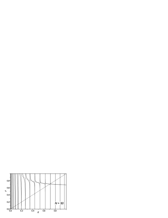
Figure 1: Graphical solution of Eqs. (13) and (14). Intersection of the $F\!=\!E$ straight line with the dotted line corresponds to the CSFE energy, $E_{\rm SF}\!\approx 0.71\!$. See text for details.

Fig. 1 shows the result of calculations for $N=50$. The lines which are restricted by vertical asymptotes reflect the result of calculation of $F(E)$. Points of singularity $E^{(i)}$, at which $F$ goes to infinity, are roots of the equation $D_{N}(E)=0$ where $D_{N}$ is the determinant corresponding to the “left-side” of the set of equations for $A_{n}$. By increasing $N$ we increase the order of equation $D_{N}(E)=0$, so that this has up to $N$ real roots. Indeed, when observing the evolution of $F(E)$ with increasing $N$, one finds that the number of singular points grows, and they become more densely placed. For $N\to\infty$ one could expect that a singular point appears within an arbitrarily small vicinity of every value $E$. Since all the vertical asymptotes $E=E^{(i)}$ are crossed by the straight line $F=E$ (see Fig. 1), we come to the conclusion that for any $E$ there is a singular solution of Eqs. (13) and (14). Such solutions with singular functions $\varphi(q)$ form a band. The physical meaning of this result is quite transparent. Namely, the band corresponds to energy ${\cal E}_{\rm sw}(q)\!+\!{\cal E}_{\rm mp}(q)$ of unbound exciton pairs. Now we only consider the solution $E=F(E)$, where the $F\!=\!E$ line crosses a conventional envelope curve tracing the regions of regularity of $\varphi_{0}$ determined by Eq. (17). Such regions at a finite $N$ should be as distant as possible from the points of singularity, and we simply define them as the vicinities of “middle” points $\overline{E}^{(i)}=\frac{1}{2}(E^{(i)}+E^{(i+1)})$. The envelope curve may obviously be defined as the line passing through the points $[\overline{E}^{(i)},\,F(\overline{E}^{(i)})]$. The intersection with the straight line $F=E$ occurs at the only point stable with respect to evolution of this picture at $N\to\infty$. This intersection point is readily seen in Fig. 1.

Fig. 1 shows the build-up of singular points (vertical lines) with vanishing $E$ and vice versa a certain rarefication of singularities in the vicinity of $E_{\rm SF}$. The former reflects growth of the density of states at the bottom of the exciton band whereas the latter is a usual effect of the “levels’ repulsion”. Note that the non-Hartree-Fock shift for the CSFE level is positive as compared to the value $E_{\rm HF}\!=\!0.627$. This is expected because the repulsion of the CSFE from the lower-lying crowded states of unbound excitons should be stronger than from the upper states having comparatively low density. At the same time, one can also see in Fig. 1 some trend towards the concentration of singularity points $E^{(i)}$ at higher energies $E$. This is evidently a consequence of the density of states growth at the top of the exciton band.

In general, the larger is $N$ the more accurate is the calculation of $\varphi_{0}(q)$ and $E$, i.e. the envelope curve in Fig. 1 becomes discernible and may be drawn only at considerable $N$. At the same time the analysis reveals that the intersection point with the $F\!=\!E$ line is rather stable and only weakly depends on $N$. This feature prompts us to consider the case $N\!=\!1$ where double-exciton states mixed with ${\cal Q}^{\dagger}_{0\overline{1}{\bf q}}|0\rangle$ are modelled by a single vector $|{\rm DX},1\rangle$. Actually the $N\!=\!1$ approximation for the problem determined by Eqs. (13), (14) and (17) is equivalent to a variational procedure for the trial double-mode state $|{X}_{0}^{\rm DM}\rangle\!=\!{\cal Q}^{\dagger}_{0\overline{1}{\bf 0}}|0\rangle\!+\!A_{1}|{\rm DX},1\rangle$, where the correlation part of the excitation energy is found from equation

$$E=\mathop{\rm min}\nolimits\limits_{A_{1}}\!\left(\frac{\langle{X}_{0}^{\rm DM}|{\hat{H}}_{\rm int}|{X}_{0}^{\rm DM}\rangle}{\langle{X}_{0}^{\rm DM}|{X}_{0}^{\rm DM}\rangle}\right)\!-\!{E}_{\rm vac}^{\rm int}\,$$

(${E}_{\rm vac}^{\rm int}$ denotes the correlation part of the ground-state energy). After minor manipulations we find that this simple double-mode approximation (DMA) reduces our problem to the secular equation $\mbox{det}\!\left|(E-{\EuScript E}_{i})\delta_{ik}+(1\!-\!\delta_{ik}){\EuScript D}_{ik}\right|\!=\!0$ (indexes $i$ and $k$ are 1 or 2), where ${\EuScript E}_{1}\!=\!\int_{0}^{\infty}\!qdqV(q)\epsilon(q),\;$ ${\EuScript E}_{2}\!=\!{\cal E}_{\rm HF},\;$ and ${}\;{\EuScript D}_{12}\!\equiv\!{\EuScript D}_{21}\!=\!\int_{0}^{\infty}\!qdqV(q)d(q)$ with $\epsilon\!=\!2q^{2}(1\!-\!q^{2})^{2}e^{-3q^{2}/2}\!+\!\frac{1}{2}(q^{2}\!-\!5q^{2}\!+\!q^{4})e^{-q^{2}}\!-\!\frac{1}{16}(q^{2}\!-\!4)^{3}e^{-3q^{2}/4}\!+\!({q^{2}}/{2}\!-\!2)e^{-q^{2}/2}$ and $d\!=\!q^{2}(q^{2}\!-\!1)e^{-q^{2}}.$ Only the largest root of this secular equation has physical meaning. In the ideal 2D case we easily obtain the DMA correlation energy of the CSFE: $E_{\rm SF}=0.766$. Comparing this result with Fig. 1 we conclude that even the DMA works rather well.

Figure 2: Main picture: DMA and HF shifts in dimensionless units against the form-factor parameter $b$. Inset: DMA shift against the magnetic field when $b\!=\!5.45\,B^{-1/2}$ ($b\!=\!0.213\,l_{B}\!/\mbox{nm},\;$ $l_{B}$ in nm’s, $B$ in Teslas); symbols are experimental data for the $25\,$nm quantum wells.va06

Fig. 2 shows the CSFE correlation energy calculated within the DMA and employing the HF approximation, if the vertex $V$ for a real 2DEG is defined as $V\!=\!F_{b}(q)/q$ with the formfactor $F_{b}(q)\!=\!\frac{1}{8}\left(1\!+\!\frac{q}{b}\right)^{-3}\left[8\!+\!9\frac{q}{b}\!+\!3\left(\frac{q}{b}\right)^{2}\right].$an82 ; lo93 Here $b=b_{0}l_{B}$ is a dimensionless parameter corresponding to dimensionless $q$. ($b_{0}$ is considered to be independent of the magnetic field.) It is seen that the non-HF shift of the CSFE energy, being about $15\%$ in the strict 2D limit (i.e., in the $b\!\to\!\infty$ case), becomes smaller ($\sim\!5-6\%$) in real samples. This difference is not observable experimentally.va06 Meanwhile, the DMA results are in good agreement with experimental data where the CSFE correlation energy is measured as a function of magnetic field, see inset in Fig. 2. The chosen value, $b_{0}\!=\!0.213/$nm, is quite consistent with the available wide quantum wells.va06

In conclusion, we note that preliminary analysis indicates that the non-HF shift should be more substantial in the case of a fractional filling, e.g. at $\nu\!=\!1/3$. Moreover, contrary to the single-mode approximation lo93 shifting the energy to lower values as compared to the HF result, the approach taking into account the double-exciton component should lead to a considerable positive shift in the CSFE correlation energy.

The authors acknowledge support of the RFBR and hospitality of the Max Planck Institute for Physics of Complex Systems (Dresden) where partly this work was carried out. The authors also thank I.V. Kukushkin, L.V. Kulik and A.B. Van’kov for the discussion.

References

• (1) T. Ando, A. B. Fowler, and F. Stern, Rev. Mod. Phys. 54, 437 (1982). The Quantum Hall Effect, Ed. by R.R. Prange and S.M. Girvin, 2nd Ed. (Springer, New York, 1990).
• (2) Yu.A. Bychkov, S.V. Iordanskii, and G.M. Eliashberg, JETP Lett. 33, 143 (1981).
• (3) Yu.A. Bychkov and E.I. Rashba, Sov. Phys. JETP 58, 1062 (1983).
• (4) C. Kallin and B.I. Halperin, Phys. Rev. B 30, 5655 (1984).
• (5) S. Dickmann, I.V. Kukushkin. Phys. Rev. B 71, 241310(R) (2005).
• (6) S.M. Dickmann, V.M. Zhilin, and D.V. Kulakovskii, JETP 101, 892 (2005).
• (7) A.H. MacDonald J. Phys. C 18, 1003 (1985).
• (8) J.P. Longo and C. Kallin, Phys. Rev. B 47, 4429 (1993).
• (9) The first-order calculations as far as the MF approach for the ${\bf q}\!=\!0$ cyclotron spin-flip plasmon at even $\nu$ give zero energy shift from the cyclotron gap $\hbar\omega_{c}$. Actually the negative shift may be found exactly by performing full perturbative calculation to the second order in $r_{\rm c}$.di05
• (10) A. Pinczuk, B.S. Dennis, D. Heiman, C. Kallin, L. Brey, C. Tejedor, S. Schmitt-Rink, L.N. Pfeiffer, and K.W. West, Phys. Rev. Lett. 68, 3623 (1992).
• (11) A.B. Van’kov, L.V. Kulik, I.V. Kukushkin, V.E. Kirpichev, S. Dickmann, V.M. Zhilin, J.H. Smet, K. von Klitzing, and W. Wegscheider. Phys. Rev. Lett., 97, 246801 (2006).
• (12) S. Dickmann, Phys. Rev. B 65, 195310 (2002).
• (13) A. B. Dzyubenko and Yu. E. Lozovik, Sov. Phys. Solid State 25, 874 (1983); ibid 26, 938 (1984); J. Phys. A 24, 415 (1991).
• (14) If using ER, the relevant operators in our case are ${\hat{H}}_{\rm ED}\!=\!\sum\limits_{a=0,\overline{0},1}\!\!\!{\hat{H}}_{a}\!+\!\!\!\!\!\sum\limits_{ab=0\overline{0},01,\overline{0}1}\!\!\!{\hat{H}}_{ab}$, where
H^a=12β€‹βˆ‘πͺV​(q)​ha​a2​(πͺ)​(𝒬a​a​πͺ†​𝒬a​a​πͺβˆ’NΟ•βˆ’1/2​𝒬a​aβ€‹πŸŽβ€ ),H^a​b=βˆ‘πͺV​(q)​[ha​a​(πͺ)​hb​b​(πͺ)​𝒬a​a​πͺ†​𝒬b​b​πͺ+|ha​b​(πͺ)|2​δσa,Οƒb​(𝒬a​b​πͺ†​𝒬a​b​πͺβˆ’NΟ•βˆ’1/2​𝒬b​bβ€‹πŸŽβ€ )]andha​b=(na!nb!)1/2​(i​qx+qy2)nbβˆ’na​Lnanbβˆ’na​(q2/2)​eβˆ’q2/4(Lij​is Laguerre polinomial).subscript^π»π‘Ž12subscriptπͺπ‘‰π‘žsuperscriptsubscriptβ„Žπ‘Žπ‘Ž2πͺsuperscriptsubscriptπ’¬π‘Žπ‘Žπͺ†subscriptπ’¬π‘Žπ‘Žπͺsuperscriptsubscript𝑁italic-Ο•12superscriptsubscriptπ’¬π‘Žπ‘Ž0†subscript^π»π‘Žπ‘subscriptπͺπ‘‰π‘ždelimited-[]subscriptβ„Žπ‘Žπ‘Žπͺsubscriptβ„Žπ‘π‘πͺsuperscriptsubscriptπ’¬π‘Žπ‘Žπͺ†subscript𝒬𝑏𝑏πͺsuperscriptsubscriptβ„Žπ‘Žπ‘πͺ2subscript𝛿subscriptπœŽπ‘ŽsubscriptπœŽπ‘superscriptsubscriptπ’¬π‘Žπ‘πͺ†subscriptπ’¬π‘Žπ‘πͺsuperscriptsubscript𝑁italic-Ο•12superscriptsubscript𝒬𝑏𝑏0†formulae-sequenceandsubscriptβ„Žπ‘Žπ‘superscriptsubscriptπ‘›π‘Žsubscript𝑛𝑏12superscript𝑖subscriptπ‘žπ‘₯subscriptπ‘žπ‘¦2subscript𝑛𝑏subscriptπ‘›π‘Žsuperscriptsubscript𝐿subscriptπ‘›π‘Žsubscript𝑛𝑏subscriptπ‘›π‘Žsuperscriptπ‘ž22superscript𝑒superscriptπ‘ž24subscriptsuperscript𝐿𝑗𝑖is Laguerre polinomial\begin{array}[]{l}{\hat{H}}_{a}\!=\!\frac{1}{2}\sum_{\bf q}\!V(q)h_{aa}^{2}({\bf q})\left({\cal Q}_{aa{\bf q}}^{\dagger}{\cal Q}_{aa{\bf q}}\!-\!N_{\phi}^{-1/2}{\cal Q}_{aa{\bf 0}}^{\dagger}\right),\\ {\hat{H}}_{ab}\!=\!\sum_{\bf q}\!V(q)\left[h_{aa}({\bf q})h_{bb}({\bf q}){\cal Q}_{aa{\bf q}}^{\dagger}{\cal Q}_{bb{\bf q}}\!+\!|h_{ab}({\bf q})|^{2}\delta_{\sigma_{a},\sigma_{b}}\left({\cal Q}_{ab{\bf q}}^{\dagger}{\cal Q}_{ab{\bf q}}\!-\!N_{\phi}^{-1/2}{\cal Q}_{bb{\bf 0}}^{\dagger}\right)\right]\\ \mbox{and}\quad h_{ab}\!=\!\left(\frac{n_{a}!}{n_{b}!}\right)^{1/2}\!\!\left(\frac{iq_{x}\!+\!q_{y}}{\sqrt{2}}\right)^{n_{b}\!-\!n_{a}}\!\!L_{n_{a}}^{n_{b}\!-\!n_{a}}(q^{2}/2)e^{-q^{2}/4}\quad(L^{j}_{i}\;\;\mbox{is Laguerre polinomial}).\end{array}
• (15) For reference we write out Eqs. (11) and (12) in the πͺβ‰ 0πͺ0{\bf q}\not=0 case:
$$\!\!\begin{array}[]{l}\left[E_{q}-{\cal E}_{\rm sw}(|{{\bf q}}/2\!-\!{{\bf p}}|)-{\cal E}_{\rm mp}(|{{\bf q}}/2\!+\!{{\bf p}}|)\right]\varphi_{q}({\bf p})\!-\!\frac{1}{\sqrt{2}}\left\{g_{q}({\bf p})\right\}{}{}{}{}\\ =(2\pi)^{-1}\int d{{\bf s}}\,\varphi_{q}({{\bf s}})\left[{\vphantom{-{\tilde{U}}_{01}(|{{\bf q}}/2+{{\bf s}}|)}}\left[U_{00}(|{{\bf p}}-{{\bf s}}|)-{\tilde{U}}_{01}(|{\bf q}/2+{\bf s}|)\right]e^{i({\bf p}\times{\bf s})_{z}}\right.{}{}\\ \left.+U_{01}(|{{\bf p}}-{{\bf s}}|)e^{i({\bf s}\times{\bf p})_{z}}-U_{00}(|{\bf p}-{\bf s}|)e^{i\left({\bf q}\times({\bf s}-{\bf p})\right)_{z}/2}\right.-\!\left.U_{01}(|{\bf p}-{\bf s}|)e^{i\left({\bf q}\times({\bf p}-{\bf s})\right)_{z}/2}{\vphantom{-{\tilde{U}}_{01}(|{{\bf q}}/2+{{\bf s}}|)}}\right]\end{array}$$
and ${}\qquad{}\qquad{}\qquad{}\qquad E_{q}={\cal E}_{0\overline{1}}(q)+\frac{1}{\pi\sqrt{2}}\int d{{\bf p}}\,g^{*}_{q}({\bf p})\varphi_{q}({\mbox{\boldmath$p$}})$ with the β€˜free’ term ${}\;\frac{1}{\sqrt{2}}\left\{g_{q}({\bf p})\right\},\;$ where $\;\,g_{q}({{\bf p}})={\tilde{U}}_{01}(|{\bf p}+{\bf q}/2|)e^{i\left({\bf p}\times{\bf q}\right)_{z}/2},\;\,$ ${\tilde{U}}_{01}\!=\!V(q)|h_{01}({\bf q})|^{2}\;\,$ and $\;U_{n_{a}n_{b}}\!=\!V(q)h^{2}_{ab}({\bf q})$ (see notations of Ref. foot2, ). If ${\bf q}$ is chosen parallel to ${\hat{y}}$, then $\varphi_{q}({\bf p})$ is an even function with respect to the replacement $p_{x}\!\to\!-p_{x}$. The HF result ${\cal E}_{0\overline{1}}(q)$ was calculated in Ref. lo93, .