Hyper-domains in exchange bias micro-stripe pattern

Abstract

A combination of experimental techniques, e.g. vector-MOKE magnetometry, Kerr microscopy and polarized neutron reflectometry, was applied to study the field induced evolution of the magnetization distribution over a periodic pattern of alternating exchange bias stripes. The lateral structure is imprinted into a continuous ferromagnetic/antiferromagnetic exchange-bias bi-layer via laterally selective exposure to He-ion irradiation in an applied field. This creates an alternating frozen-in interfacial exchange bias field competing with the external field in the course of the re-magnetization. It was found that in a magnetic field applied at an angle with respect to the exchange bias axis parallel to the stripes the re-magnetization process proceeds via a variety of different stages. They include coherent rotation of magnetization towards the exchange bias axis, precipitation of small random (ripple) domains, formation of a stripe-like alternation of the magnetization, and development of a state in which the magnetization forms large hyper-domains comprising a number of stripes. Each of those magnetic states is quantitatively characterized via the comprehensive analysis of data on specular and off-specular polarized neutron reflectivity. The results are discussed within a phenomenological model containing a few parameters which can readily be controlled by designing systems with a desired configuration of magnetic moments of micro- and nano-elements.

I Introduction

The exchange bias (EB) effect, which is due to exchange coupling between ferromagnetic (F) and antiferromagnetic (AF) layers, is expressed via a shifted hysteresis loop away from zero field. The shift is attributed to the frozen-in global unidirectional anisotropy of the system. Due to its intriguing physics and importance for device application the EB effect is persistently under extensive study (see Refs. Nougues ; Berkowitz ; Stamps ; Kiwi ; Nogues_nano ). Spacial alteration of the EB field brings qualitatively new physics into EB systems and creates new promising technological perspectives. Deep understanding of the role of competing interactions in this class of materials is required e.g. to manufacture F/AF films with imprinted in-plane ferromagnetic domain pattern with desired morphology. One of the motivations is to design planar magnetic patterning of a continuous film as an alternative to magnetic grains, clusters or structures patterned by lithographic methods. With such systems one could avoid the problem of very small feature sizes, where the long-term thermal stability of the magnetic elements is lost due to superparamagnetic fluctuations Moser .

The EB effect is usually set via cooling the system below the blocking temperature of the AF layer in a magnetic field saturating the ferromagnetic counterpart. The size and the sign of the EB effect depends on the choice of F/AF materials in contact and often can be altered via changing the field cooling protocol Suess ; Hong ; Ohldag . On the other hand, the EB field direction and strength can be selectively altered by ion bombardment of the F/AF bi-layer subjected into an external field of the opposite direction Schmalhorst ; Engel . Depositing a grid protecting some areas of the sample one can preserve the EB field in those areas, while altering its direction in the unprotected regions. The method of Ion Beam Induced Magnetic Patterning (IBMP) Ehresmann_rev opens wide perspectives to produce various EB patterns. Here we report on the magnetic properties of a IBMP produced stripe-like pattern with the EB-field set antiparallel in neighboring stripes so that the net EB field is compensated and the system should posses global uniaxial, instead of unidirectional, anisotropy. Therefore it is expected that the ferromagnetic stripe domains in such a system display alternating magnetization directions in the remanent demagnetized state of the sample. Details on the sample preparation and the results of experimental and theoretical studies of the magnetization reversal mechanism of the system for the field applied along the exchange bias axis can be found in our recent publication Theis-Broehl_PRB2006 . There by use of the magneto-optical Kerr-effect (MOKE) in vector-MOKE configuration, Kerr microscopy and polarized neutron reflectometry (PNR) it has been shown that the system exhibits a hysteresis rich in details and with a complex domain structure. Surprisingly, it was found that in the easy axis configuration the magnetic state after reversal of one of the both types of stripe domains never shows a clear antiparallel domain structure. Instead, at low fields the magnetization in the different EB stripes is periodically canted with respect to the EB axis so that alternating antiparallel ordering of domain magnetization projections onto the stripe axis co-exists with a macroscopic magnetic moment perpendicular to the anisotropy axis. This effect is explained within the framework of a simple phenomenological model which takes into account competing interfacial and intralayer exchange interactions. According to the model, within a certain range of parameters including, e.g. the ratio between ferromagnetic layer thickness and the stripe width, the system reveals an instability with respect to the tilt of magnetization to the left, or to the right against the EB stripe induced anisotropy axis. In our previous study Theis-Broehl_PRB2006 it is always found flipped only in one of two nominally equal directions so that the system always carried an appreciable residual magnetization not collinear with the anisotropy axis and the magnetic field.

The finding in Ref. Theis-Broehl_PRB2006 may have more general and far going consequences for the understanding of the inherent physics of the EB effect. Areas with alternating EB fields must exist in any F/AF bi-layers coupled via exchange interaction through a common atomically rough interface Malozemoff_1987 ; Malozemoff_1988 . Alternating interfacial fields in this case are generated by uncompensated spins in AF areas in neighboring atomic steps which are shifted up or down with respect to each other for half of the magnetic unit cell of the Ising type antiferromagnet. Those interfacial fields randomly alternate over the F/AF interface and compete with the lateral exchange interaction which favors a homogeneously magnetized ferromagnetic film. Depending on film thickness and strength of the interactions, e.g. the interfacial F/AF vs lateral exchange in the ferromagnetic film, the competition may result in a state with magnetization of the Heisenberg ferromagnet (inhomogeneously) tilted away from the external field applied collinearly with EB direction. In view of that the magnetization distribution in the model system with a controlled EB field alternation deserves further comprehensive consideration.

First of all we admit that the previously observed Theis-Broehl_PRB2006 preferential large tilt of the net magnetization away from the symmetry axis can be explained by a tiny misalignment between frozen-in EB fields in irradiated and protected stripes. Such a misalignment determines a preferential direction of the small net EB field noncollinear with stripes. In the vicinity of the instability point the net magnetization naturally appears in the direction of this field. It is quite a challenging technological task to set both EB fields exactly antiparallel and collinear with the stripes. This is not a goal of the present paper, where instead, we report on the results avoiding this problem by an deliberate tilt of the external field direction by an angle as high as 45^∘ regarding to the anisotropy axis set along the stripes. Then a little misalignment between the EB fields in neighboring stripes plays a minor role. Measurements in an asymmetric regime, on the other hand, disclose many details on domain organization and evolution which are otherwise hidden, but absolutely crucial for a complete understanding of the re-magnetization mechanisms in EB patterned arrays and other types of systems with alternating EB fields. The bulk of information is mostly gained via the quantitative analysis of data on PNR. The scattering intensity distribution was measured over a broad range of angles of incidence and scattering and accomplished with a full polarization analysis at different magnetic fields along the hysteresis loop. For fitting the specular reflectivity data we used an originally developed least-squares software package, Deriglazov which allows for simultaneous evaluation of all four measured reflectivities in one cycle. We compare the results of our fits to vector-MOKE measurements. For supporting the interpretation of our data on off-specular diffuse and Bragg scattering Kerr-microscopy (KM) images McCord were also taken.

II Experimental Details

The sample studied is a TaO-Ta(8.7 nm)/ Co₇₀Fe₃₀(28.0 nm)/ Mn₈₃Ir₁₇(15.2 nm)/ Cu(28.4 nm)/ SiO₂(50.5 nm)/ Si(111) film stack. The initial EB direction was set by field cooling in a magnetic in-plane field of 100 mT after an annealing step for 1 h at 275 ^∘C which is above the blocking temperature of the antiferromagnetic material. Subsequently, IBMP using He⁺ ions with a fluency of $1\times 10^{15}$ ions/cm² at 10 keV was applied at a magnetic field of 100 mT aligned opposite to the initial EB direction. This resulted in a stripe-like domain pattern of equally spaced stripes with a width of $2.5~{}\mu$m and a periodicity of $\Lambda=5~{}\mu$m and with alternate sign of the unidirectional anisotropy, and hence of the EB in neighboring stripes.

The evolution of magnetization as a function of applied field was recorded with a vector-MOKE setup as described in Ref. Schmitte . Both magnetization projections were accessed via measuring the Kerr angle parallel and perpendicular to the field. The projections were measured in the longitudinal MOKE configuration, i.e. with the incident light linearly polarized within the reflection plane. For determination of the magnetization component perpendicular to the field the sample and the magnetic field direction were rotated simultaneously by 90^∘ about the normal to the surface. Assuming that the Kerr angles, $\theta_{\mathrm{K}}^{\mathrm{L}}\propto M\cos{\overline{\gamma}}$, measuring the magnetization vector projection and the Kerr angle parallel to the field, and $\theta_{\mathrm{K}}^{\mathrm{T}}\propto M\sin{\overline{\gamma}}$, corresponding to the perpendicular magnetization component, have the same proportionality coefficients, one can determine the tilt angle $\overline{\gamma}$ through $\tan\overline{\gamma}={\theta_{\mathrm{K}}^{\mathrm{T}}}/{\theta_{\mathrm{K}}^{\mathrm{L}}}$ and the normalized length of the magnetization vector $M/M_{\mathrm{s}}={\sqrt{(\theta_{K}^{L})^{2}+(\theta_{K}^{T})^{2}}}/{\theta_{K}^{\mathrm{s}}}$ with $M_{\mathrm{s}}$ being the modulus of the magnetization and $\theta_{K}^{\mathrm{s}}$ the Kerr angle, both in saturation. This allows to completely determine the direction of the mean magnetization vector $M$ and its absolute value $M=|{\bf\mbox{\boldmath$M$}}|$ reduced due to domains. In different domains the magnetization vector deviates by angles $\Delta\gamma$ from the direction of the mean magnetization and hence is tilted by $\gamma=\overline{\gamma}+\Delta\gamma$ against the applied field. The mean angle $\overline{\gamma}$ is determined by the equation $\langle\sin\Delta\gamma\rangle_{\mathrm{coh}}=0$, where the averaging runs over the spot coherently illuminated by the laser beam. Then the normalized longitudinal and, correspondingly, transverse MOKE signals can be written as:

$$\langle\cos\gamma\rangle_{\mathrm{coh}} = M/M_{s}\cos\overline{\gamma}=\langle\cos\Delta\gamma\rangle_{\mathrm{coh}}\cos\overline{\gamma},$$ (1)

$$\langle\sin\gamma\rangle_{\mathrm{coh}} = M/M_{s}\sin\overline{\gamma}=\langle\cos\Delta\gamma\rangle_{\mathrm{coh}}\sin\overline{\gamma},$$ (2)

where the mean magnetization $M=M_{s}\langle\cos\Delta\gamma\rangle_{\mathrm{coh}}$.

Further insight into the microscopic rearrangement of magnetization was achieved by a high resolution magneto-optical Kerr microscope (KM) HubertSchaefer that is sensitive to directions orthogonal to the field McCord .

Neutron scattering experiments were carried out with the HADAS reflectometer at the FRJ-2 reactor in Jülich, Germany. Details of the measuring geometry can be found in Ref. Theis-Broehl_PRB2006 . In the present experiment the sample was aligned so that the field orientation was tilted by $45^{\circ}$ against the EB axis. The monochromatic neutron beam with the wavelength of $0.452$ nm incident onto the sample surface under the glancing angle $\alpha_{i}$ is scattered under the angle $\alpha_{f}$, so that for specular reflection $\alpha_{f}=\alpha_{i}$. The incident polarization vector ${\mbox{\boldmath$P$}}_{i}$ was directed either parallel or antiparallel to the magnetic field and perpendicular to the scattering plane. In each of the two directions of ${\mbox{\boldmath$P$}}_{i}$ the final spin state was analyzed with respect to the same direction with an efficiency $P_{f}=|{\mbox{\boldmath$P$}}_{f}|\leq 1$.

Specular PNR provides information similar but not identical to vector-MOKE magnetometry. Both methods probe projections of the magnetization vector averaged over its deviations due to magnetic domains and other inhomogeneities within the coherence volume of photons, or neutrons, respectively. In the case of MOKE the laser beam is rather coherent all over the isotropic light spot illuminating the sample surface. This is not the case for PNR. The neutron source is essentially incoherent, but the neutron beam is well collimated in the reflection plane, while the collimation is usually relaxed perpendicular to this plane. Hence the cross section of the coherence volume with the reflecting surface is represented by an ellipsoid with dramatically extended axis along the beam projection onto the surface. At shallow incidence this extension, i.e. the longitudinal coherence length, may spread up to some fractions of a millimeter. In contrast, the other ellipsoid axis, i.e. the coherence length across the incoming beam is short and only amounts to about 10 nm. Therefore, the coherence 2D ellipsoid covers only a very small area of the sample, and the observed PNR signal is a result of two sorts over averaging. The first one includes a coherent averaging of the reflection potential, e.g. over directions of the magnetization in small (periodic and random) domains, and runs over the coherence area. Second, the reflected intensities from each of those areas are summed up incoherently.

If the mean magnetization averaged over the coherence area is nonzero and collinear with the external field (applied parallel to the neutron polarization axis and perpendicular to the scattering plane) then specular reflection does not alter the neutron spin states and only two non-spin-flip (NSF) reflection coefficients ${\mathcal{R}}^{+\,+}\neq{\mathcal{R}}^{-\,-}$ are measured, while both spin-flip (SF) reflectivities ${\mathcal{R}}^{+\,-}={\mathcal{R}}^{-\,+}=0$. In this case NSF reflectivities are uniquely determined by the mean optical potential, e.g. by the mean projection of the magnetization proportional to $\langle\cos\Delta\gamma\rangle_{\mathrm{coh}}$, where $\Delta\gamma$ is the tilt angle of the magnetization in domains smaller than the coherence length .

If the mean magnetization direction makes an angle $\overline{\gamma}=\langle\gamma-\Delta\gamma\rangle_{\mathrm{coh}}$ with the applied field then the SF reflectivities ${\mathcal{R}}^{+\,-}={\mathcal{R}}^{-\,+}\neq 0$ and are proportional to $\sin^{2}\overline{\gamma}$, i.e. to the mean square of the magnetization projection normal to the field. At the same time the difference, ${\mathcal{R}}^{+\,+}-{\mathcal{R}}^{-\,-}$, between the NSF reflectivities is proportional to $\cos\overline{\gamma}$, i.e. to the projection of the mean magnetization within the coherence volume onto the applied field direction. Crossing a number of small periodic and random domains in only one direction the coherence ellipsoid still covers a very small area of the sample. Therefore, the angle $\overline{\gamma}$ may vary along the sample surface and reflectivities have to be incoherently averaged over the spread of $\overline{\gamma}$. It is important to note that NSF and SF reflectivities are complicated nonlinear functions of $\langle\cos\Delta\gamma\rangle_{\mathrm{coh}}$, which may also vary along the sample surface. Hence, such an averaging is, in general, not a trivial procedure.

If the value of $\langle\cos\Delta\gamma\rangle_{\mathrm{coh}}$ is, however, unique Theis-Broehl_PRB2006 for the whole sample surface, then

$${\mathcal{R}}^{+\,+} - {\mathcal{R}}^{-\,-}\propto\langle\cos\overline{\gamma}\rangle_{\mathrm{inc}}$$ (3)

$${\mathcal{R}}^{+\,-} = {\mathcal{R}}^{-\,+}\propto\langle\sin^{2}\overline{\gamma}\rangle_{\mathrm{inc}}$$ (4)

are respectively proportional to $\cos\overline{\gamma}$ and $\sin\overline{\gamma}$ incoherently averaged over the reflecting surface with the proportionality coefficients nonlinearly depending on $\langle\cos\Delta\gamma\rangle_{\mathrm{coh}}$. Because of nonlinearity the parameters $\langle\cos\overline{\gamma}\rangle_{\mathrm{inc}}$, $\langle\sin^{2}\overline{\gamma}\rangle_{\mathrm{inc}}$ and $\langle\cos\Delta\gamma\rangle_{\mathrm{coh}}$ can only be found via fitting of the data for all NSF and SF reflectivities. After that one can determine the mean value $\langle\cos\gamma\rangle\approx\langle\cos\overline{\gamma}\rangle_{\mathrm{inc}}\langle\cos\Delta\gamma\rangle_{\mathrm{coh}}$, under the condition: $\langle\sin\Delta\gamma\rangle_{\mathrm{coh}}=0$. This constraint is similar to that applied above for vector-MOKE and hence the mean magnetization projection onto the field direction is in this case equally measured by both methods: MOKE and PNR. Then agreement between results of PNR and vector-MOKE can be used to prove the assumption above. Alternatively, PNR is able to deliver an important information complementing vector-MOKE data.

Due to the strong anisotropy of the coherence ellipsoid PNR can probe a variation of $\overline{\gamma}$ in the corresponding direction measuring fluctuations of the magnetization not accessible for MOKE. In particular, with PNR one gains a direct access to the dispersion $\Sigma^{2}=\langle\sin^{2}\overline{\gamma}\rangle_{\mathrm{inc}}-\langle\sin\overline{\gamma}\rangle_{\mathrm{inc}}^{2}\geq 0$ which quantifies those fluctuations. If, for instance, $\Sigma=0$ these fluctuations are absent, then at $\langle\sin^{2}\overline{\gamma}\rangle_{\mathrm{inc}}=\langle\sin\overline{\gamma}\rangle_{\mathrm{inc}}^{2}\neq 0$ the homogeneous sample magnetization is homogeneously tilted by the angle $\overline{\gamma}$ to the left, or to the right with respect to the applied field. PNR is not sensitive to the sign of $\overline{\gamma}$, which can be determined via vector-MOKE. On the other hand, MOKE cannot provide any information about, e.g. the totally demagnetized structure when $\langle\sin\overline{\gamma}\rangle=\langle\cos\overline{\gamma}\rangle=0$. In this case missing information can readily be retrieved from the PNR data. This can already be seen considering two limiting situations. The limiting value $\Sigma=1$ is achieved in the state with large domains where the magnetization is perpendicular to the applied field. The other limit $\Sigma=0$ is reached if demagnetization occurs on a scale smaller than the coherence area. In the latter case specular reflection is accompanied by off-specular scattering.

Off-specular PNR can, in contrast to MOKE, directly measure the spread of magnetization directions due to domains crossed with the long axis of the coherence ellipsoid. Periodic deviations $\Delta\gamma$ give rise to Bragg diffraction, while random fluctuations cause diffuse scattering. The positions of the Bragg peaks in the reciprocal space determine the period of the domain structure along the largest coherence axis, while the extension of diffuse scattering is due to the correlations of the random component of the magnetization. Via fitting of intensities of off-specular scattering one can deduce the magnetization distribution between neighboring stripe domains and in addition to $\langle\cos\Delta\gamma\rangle_{\mathrm{coh}}$ to determine one more parameter, $\langle\sin^{2}\Delta\gamma\rangle_{\mathrm{coh}}$, characterizing magnetization fluctuations due to random ripple domains. Then one can also calculate the dispersion $\sigma^{2}=\langle\cos^{2}\Delta\gamma\rangle_{\mathrm{coh}}-\langle\cos\Delta\gamma\rangle_{\mathrm{coh}}^{2}\geq 0$ quantifying the microscopic arrangement of magnetization fluctuations within the coherence length.

Often, the set of parameters indicated above is not sufficient to describe experimental data of PNR and to infer from it a domain state. Such a situation takes place when the mean value $\langle\cos\Delta\gamma\rangle_{\mathrm{coh}}$ averaged over the coherence range varies along the sample surface. Then incoherent averaging must take into account that specular reflection and off-specular scattering occur from areas with different optical potentials. As we shall see below, within a certain range of applied fields the magnetization in our system evolves via formation of large (hyper-) domains comprising a number of small stripe and ripple domains. In contrast to the case of the conventional domain state, now the magnetization in different hyper-domains differs not only in directions, but also in absolute values. This is due to the fact that each type of hyper-domains is characterized by a particular arrangement of the magnetization over stripe and ripple domains belonging to this type. Each of them acquires its own set of parameters, e.g. $\langle\cos\Delta\gamma_{j}\rangle_{\mathrm{coh}}$, $\langle\sin^{2}\Delta\gamma_{j}\rangle_{\mathrm{coh}}$, $\langle\cos\overline{\gamma}_{j}\rangle_{\mathrm{inc}}$ and $\langle\sin^{2}\overline{\gamma}_{j}\rangle_{\mathrm{inc}}$, where the superscript $j$ indexes the type of hyper-domain. ${\mathcal{R}}_{j}^{\pm\pm}$, and SF, ${\mathcal{R}}_{j}^{\pm\mp}$, reflectivities, as well as cross sections of off-specular scattering, are also to be indexed accordingly. Then the weights $w_{j}$ of different types of hyper-domains can be determined along with the above listed parameters via the fitting of experimental data. This would allow to totally characterize the magnetic states of the system passing through along the hysteresis loop.

III Experimental Results

III.1 Vector-MOKE

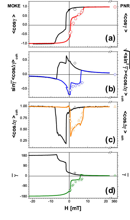
Figure 1: (Color online) Vector-MOKE data and results of fits to the PNR data. (a) Normalized hysteresis loop of the longitudinal magnetization component, (b) normalized hysteresis loop of the transverse magnetization component, (c) normalized value of the length of the magnetization vector, and (d) mean value of the angle between magnetization and external field. The field is applied at $45^{\circ}$ with respect to the EB axis. Lines represent MOKE and symbols PNR data. The symbols represent the results of the the weighted average between first and second domain (see text). The ascending curve is drawn in color and the descending one in black.

The evolution of two Cartesian projections of the normalized to saturation mean magnetization vector ${\bm{m}}={\bm{M}}/M_{\mathrm{sat}}$ determined with vector-MOKE is depicted in Fig. 1(a) and (b). Fig. 1 (c) and (d) illustrate the field dependence of the absolute value $m=\left|{\bm{m}}\right|$ of the normalized magnetization vector ${\bm{m}}$ and its tilt angle $\overline{\gamma}$ with respect the field applied at the angle of $45^{\circ}$ relative to the stripes axis. Comparing these plots one can admit several stages of the re-magnetization process as visualized in Fig. 2. Reduction of the negative field from saturation leads firstly to relatively slow coherent rotation of the magnetization vector away from the field direction while maintaining its absolute value [Fig. 2 (a)]. At small positive field $H=H_{c1}\approx 0.6$ mT this process is suddenly interrupted apparently due to domain formation [Fig. 2 (b)]. This stage of the process is completed at $H\approx+1.4$ mT when the magnetization loss is about half of its magnitude. At further increase of the applied field the magnetization partially restores its magnitude up to almost 63% of the nominal value. At the same time the mean magnetization vector is directed at an angle $\overline{\gamma}\approx 35^{\circ}$ with respect to the applied field [Fig. 2 (c)]. Within quite a broad interval of fields the system stays in a relatively rigid state with the mean magnetization directed almost normal to the stripes. The next dramatic event occurs at $H_{c}2$ between $H\approx 5.5$ mT and $H\approx 7.0$ mT when the magnetization again looses and partially restores its absolute value [Fig. 2 (d)]. Within this stage the vector ${\bm{m}}$ rapidly starts to rotate towards the magnetic field direction and is aligned along the field at $H\approx 6.0$ mT. At higher fields the magnetization, surprisingly, continues to rotate further away from the field direction and at $H\approx 6.5$ mT it arrives at a maximal tilt angle $\overline{\gamma}\approx 9^{\circ}$. This stage of the the re-magnetization process is apparently governed by a domain re-arrangement mechanism which restores the magnetization absolute value up to about 65% of its nominal. Rapid restoration of magnetization follows, presumably, through an additional intermediate stage of domain evolution within the field frame $7.0\leq H\leq H_{sat}$ [Fig. 2 (e)].

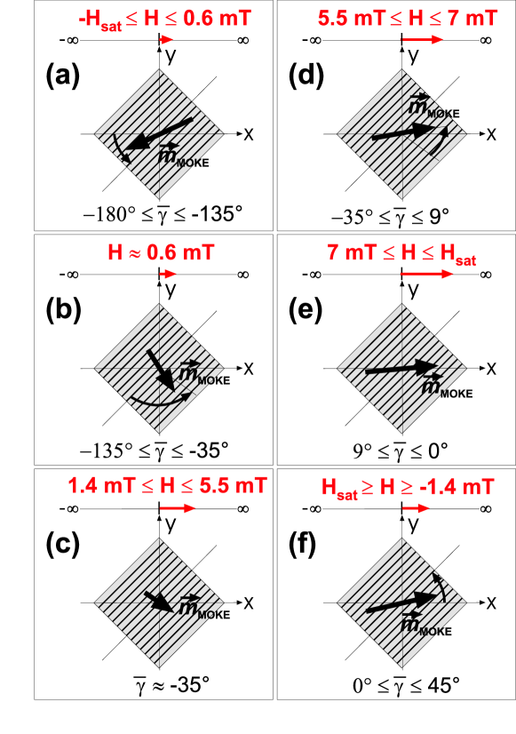
Figure 2: (Color online) Evolution of the mean magnetization along the MOKE hysteresis loop.

The descending branch of the hysteresis loop [the first stage is shown in Fig. 2 (f)] generally repeats all main steps of the magnetization evolution. However, the magnetization vector does not passes them in the exactly reversed order, as would be expected. Instead, along the descending branch the vector ${\bm{M}}$ continues to rotate in the same direction passing by the state with the magnetization along the field as in the case of the ascending branch of the hysteresis loop. Finally the vector ${\bm{m}}$ accomplishes the full circle of $360^{\circ}$ and then slightly rotates back approaching negative saturation. The intrinsic reason of such a behavior should find its explanation below after more detailed analysis of the complete scope of the data.

Here we just mention that the hysteresis loops are shifted exhibiting a global EB effect and hence a residual frozen-in magnetic field. This indicates an incomplete compensation of fields frozen-in different sets of stripes. Further insight into the arrangement of magnetization over stripes is gained by use of Kerr microscopy.

III.2 Kerr microscopy

A sequence of KM images taken along the hysteresis loop for the present sample with the field applied along the exchange bias axis, perpendicular, and at $45^{\circ}$ to this axis were briefly reported recently McCord . It was demonstrated, that in the latter case the evolution of the magnetization distribution recorded in the images, e.g. in those presented in Fig. 3, elucidates the role of various mechanisms involved in the re-magnetization process according to the typical stages of the re-magnetization process shown in Figs. 2 (a-f). Figs. 3(a-e) illustrate the re-magnetization scenario along the ascending branch after saturation in a negative field. Fig. 3(a) shows a measurement performed at a small positive field of 0.3 mT. At this field the magnetization already appreciably deviates from the field axis but it is not yet reversed in neither of the stripes. The periodic KM contrast indicates an angle between the directions of magnetization in neighboring stripes. Some rippling, predominantly in the He⁺ bombarded regions, can also be observed. At 0.6 mT [Fig. 3(b)] the reversal occurs through the formation of large hyper-domains separated along one of the stripes. In one of such hyper-domains the magnetization of the stripes is not yet reversed. In the other hyper-domain the magnetization in one set of stripes, i.e. in this case in the He⁺ bombarded, is reversed as seen via a large optical contrast. At 1.4 mT no hyper-domains are seen and the magnetization projections onto the EB axis in neighboring stripes seems to be aligned antiparallel [Fig. 3 (c)]. Further increase of the applied field changes the scenario of the re-magnetization process, as seen in Figs. 3 (d) and (e). Now it proceeds through gradual decrease of the width of stripes with the most unfavorable magnetization direction. Fig. 3 (f) was taken in the backward branch. It shows that reappearance of the continuous stripes with a negative projection onto the field direction is preceded by precipitation of small ripple domains. Further decrease of the positive field and its subsequent alternation restores the periodic structure via coalescence of ripple domains in corresponding sets of stripes McCord . This process, however, does not occur simultaneously all over the sample surface, but again involves the formation of hyper-domains. Some of them contain homogeneously magnetized stripes, while in the others the magnetization of one set of stripes is broken into ripple domains.

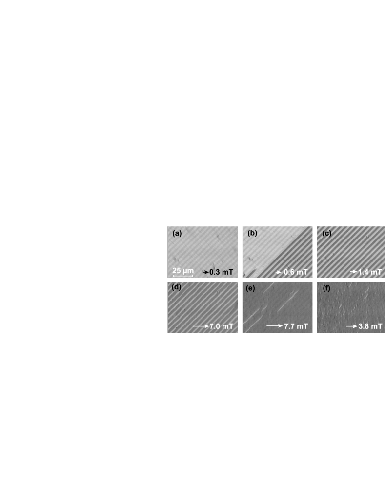
Figure 3: Kerr microscopy images taken during the magnetization reversal with the field aligned diagonally to the EB axis. The images were recorded with a mixed Kerr sensitivity tuned nearly to the transverse magnetization direction.

It should be noted that KM images sample, in contrast to vector-MOKE and PNR, quite a restricted area of the surface. They provide, however, a rather solid background necessary for a quantitative analysis of PNR data and consequent characterization of magnetization distribution between stripe, ripple and hyper-domains over the whole sample.

III.3 Neutron scattering

Neutron scattering experiments were performed using a position sensitive detector (PSD). The PSD records, additionally to the specular reflection from the mean neutron optical potential, magnetic Bragg diffraction from the periodic stripe array and off-specular diffuse scattering from domains smaller than the long axis of the coherence ellipsoid. The data were taken at several positive field values of the hysteresis. The magnetic field was kept parallel to the field guiding the neutron polarization in order to avoid neutron depolarization. Prior to the measurements, the sample was saturated in a negative field. Specular reflectivities were extracted from the PSD maps. In Fig. 4, several representative experimental curves together with fits to the data are displayed. Most of the presented data are collected at fields corresponding to the KM images in Fig. 3. This allows for a qualitative interpretation of the specular reflectivity curves along with the KM measurements in Fig. 3.

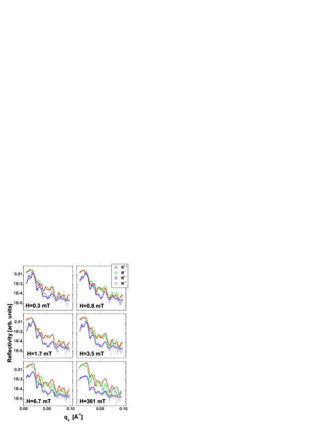
Figure 4: (Color online) Polarized neutron reflectivity measurements performed at different magnetic fields applied at the angle $\chi=45^{\circ}$ with respect to the EB axis. The symbols present measurements of non-spin flip reflectivities ${\mathcal{R}}^{+\,+}$ and ${\mathcal{R}}^{-\,-}$ and spin flip reflectivities ${\mathcal{R}}^{+\,-}$ and ${\mathcal{R}}^{-\,+}$. The lines represent fits to the data points.

At 0.3 mT splitting of the NSF reflectivities with ${\mathcal{R}}^{-\,-}$ being higher than ${\mathcal{R}}^{+\,+}$ and considerable SF reflectivities indicate an appreciable tilt of the net magnetization, almost homogeneous in accordance with Fig. 3 (a), away from the direction antiparallel to the applied field.

At 0.8 mT the SF reflectivity is slightly increased and the splitting of the NSF reflectivities is reduced compared to 0.3 mT. This is attributed to a further increasing tilt of magnetization and reduction of its absolute value due to stripe domains seen in Fig. 3 (b).

At 1.7 mT the splitting of the NSF reflectivities almost vanishes. This qualitatively can be explained by a large angle between magnetization directions in neighboring stripes. At the same time the SF reflectivity attains a maximum value manifesting a large projection of the mean magnetization component normal to the field as seen in Fig. 1. Hence, already qualitative analysis of the specular PNR and MOKE data let us conclude that the magnetization vectors in neighboring stripes in Fig. 3 (c) are not collinear with either the magnetic field or the EB axis and make quite a large angle between themselves. This angle can precisely be determined via the quantitative analysis of the complete scope of the PNR data.

We have undertaken further PNR measurements at 2.2 mT (not shown here) and 3.5 mT. At 3.5 mT increased splitting of the NSF and reduced SF reflectivities may indicate that the mean magnetization now turns towards the direction of the applied field. This conclusion, however, seems to contradict the MOKE data in Fig. 1 which do not show a substantial rotation of the mean magnetization within this interval of fields. Subsequent quantitative PNR analysis removes the contradiction between the vector-MOKE observations and the PNR analysis based on intuitive arguments.

Further PNR measurements at 5.3 mT (not shown), 6.7 mT and 7.1 mT (not shown) exhibit a continuous increase of the splitting of the NSF and a reduction of the SF reflectivities. The situations at 6.7 mT and 7.1 mT are comparable with the KM measurement in Fig. 3 (d) showing gradual shrinking and final collapse of the set of stripes with unfavorable magnetization. The SF reflectivities are already smaller as compared to the situation before the first reversal at 0.3 mT. Taking a closer look, one can also admit a number of particular details distinguished in different plots for PNR, and in particular, those recorded at 0.3 and 7.1 mT. It is rather difficult to guess a physical meaning for most of the changes in the PNR $q-$dependencies. Nonetheless, the least square routine, as we shall see, allows us to infer a variation of a few field dependent parameters quantifying KM and MOKE observations.

The major part of irrelevant parameters, e.g. those independent of the applied field are fixed via fitting the data collected at 361 mT, assuming the system at this field is in saturation. The maximum splitting seen in the last plot in Fig. 4 for the NSF reflectivities indicates that the magnetization is aligned along the applied field. Little SF reflectivity is observed due to a not perfect efficiency of the polarization device and taken into account in the subsequently applied least square routine. We also performed a measurement at a positive field of 3.1 mT in the backwards branch. It still shows a strong splitting of NSF but an increased SF reflectivity compared to saturation indicating a tilted magnetization.

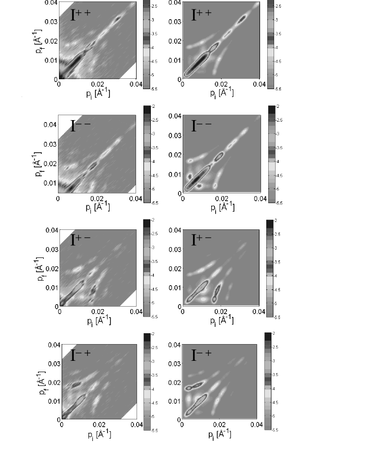
Figure 5: (Color online) Experimental (left column) maps for the polarized neutron scattering intensity on a logarithmic scale, measured at a magnetic fields of 6.7 mT. The intensities of the $I^{+\,+}$, $I^{-\,-}$ non-spin-flip, and the intensities of the $I^{+\,-}$, $I^{-\,+}$ spin-flip cross-sections are plotted as a function of the angle of incidence $\alpha_{i}$, and the scattering angle $\alpha_{f}$. Left column represents respective maps calculated in DWBA.

The most complete information on the microscopic arrangement of magnetization is, however, obtained by analyzing not solely the specular reflection, but in accordance with off-specular scattering. Figure 5 displays experimental data (left column) along with the results of theoretical simulations (right column) for all four scattering cross sections $I^{+\,+}$, $I^{-\,-}$, $I^{+\,-}$, and $I^{-\,+}$ collected into a set of maps. The scattering intensities are plotted as functions of the normal to the surface components $p_{i}=k\sin\alpha_{i}$ and $p_{f}=k\sin\alpha_{f}$ of, correspondingly, incoming, ${\bm{k}}_{i}$, and outgoing, ${\bm{k}}_{f}$, wave vectors impinging onto the surface at glancing angles of incidence, $\alpha_{i}$, and scattered at angles $\alpha_{f}$. The maps were obtained for all fields listed in Fig. 4 and in the text above but here we present only those constructed for one field at 6.7 mT and containing all features significant for the subsequent quantitative analysis. In the maps the specular reflection ridge runs along the diagonal, where $p_{i}=p_{f}$. At $p_{i}\neq p_{f}$ the scattering maps exhibit two other remarkable features. The first one is the intensity of Bragg diffraction concentrated along curved lines $q_{\parallel}\approx(2\pi n/\Lambda)\cos\chi$, where $q_{\parallel}=(2\pi/\lambda)(\cos\alpha_{i}-\cos\alpha_{f})$, $n$ denotes the order of diffraction, $\Lambda$ is the period, and $\chi$ is the angle between the stripe axis and the normal to the reflection plane . Bragg scattering occurs due to the periodic variation of the magnetization across the striped pattern and, in particular, due to the periodic alteration of the sign of $\langle\cos\Delta\gamma\rangle_{\mathrm{coh}}$ in neighboring stripes. The diffracted intensity vanishes in saturation (not shown here) and should reach maximum values in the field range where antiparallel alignment of the magnetization in neighboring microstripes is expected. The second feature is well-structured intensity of diffuse scattering observed at low angles of incidence $\alpha_{i}$ and/or scattering $\alpha_{f}$. Both features are due to the lateral magnetization fluctuations on a scale smaller than the coherence range.

In Fig. 5, strong Bragg reflections for $n=\pm 1$ and weaker ones for $n=\pm 2$ can be recognized. The observation of second-order Bragg reflections is quite a striking result. In the case of perfect alternation of magnetization projections in neighboring stripes of equal widths Bragg reflections of all even orders should be heavily suppressed due to the AF structure factor. Hence reflection of the second order was never observed in our previous measurements Theis-Broehl_PRB2006 carried out at $\chi=0$. In the present case of $\chi=45^{\circ}$ one of the KM images in Fig. 5, e.g. at $H\approx 7.0$ mT, clearly indicates a difference in the widths of neighboring stripes. This difference violates the cancellation law for the Bragg reflection of the even order . Interestingly, second-order reflections can be observed not only when they are expected from the corresponding KM image in Fig. 5, but rather at all fields along the ascending branch below saturation. In view of this, one should admit that the cancellation law requires a perfect reciprocity between magnetic moments of neighboring stripes. It can be violated not only because of a difference in the stripe widths, but also due to non-perfect alternation of stripe magnetization projections. This is particularly the case if the magnetic field is applied at an angle $\chi\neq 0$ with respect to the main symmetry axis. Then, in contrast to the symmetric case $\chi=0$, Theis-Broehl_PRB2006 the external field tilts the magnetization vector by the angle $\Delta\gamma=\beta_{1}$ in one set of stripes, or by $\Delta\gamma=\beta_{2}$ in the other set. In the asymmetric case $\chi\neq 0$ there is no reason to expect that $\beta_{1}=-\beta_{2}$, while at $\beta_{1}\neq-\beta_{2}$ neither of the stripe magnetization projections perfectly alternate.

Bragg reflections are observed in all four, SF and NSF, channels. The SF maps show a strong asymmetry with respect to the interchange $p_{i}$ with $p_{f}$ corresponding to parity between Bragg reflections with indexes $n$ and $-n$. The asymmetry is explained by the birefringence toperverg99 in the mean optical potential and is accounted for within the framework of the distorted wave Born approximation (DWBA) toperverg02 ; zabel07 . In the symmetric case ($\chi=0$) $\beta_{1}=-\beta_{2}$ and only the magnetization vector components collinear with the stripes alternate Theis-Broehl_PRB2006 . Then the SF diffraction is a result of the superposition of two effects: Bragg diffraction due to periodical alternation of the scattering potential and a homogeneous transverse magnetization which mixes up neutron spin states. This superposition is described in DWBA. In the present arrangement $\chi\neq 0$ both in-plane projections of the stripe magnetization vectors alternate, providing either NSF and SF Bragg diffraction already in the Born approximation. However, an accurate balance between intensities in all channels as well as between specular and Bragg diffraction is only possible to account for accurately in DWBA.

In Fig. 5 we also observe diffuse off-specular scattering, which is due to random fluctuations $\Delta\beta_{1}$ and $\Delta\beta_{2}$ around their mean values $\overline{\beta}_{1}$ and $\overline{\beta}_{2}$, respectively. The SF diffuse scattering is also strongly asymmetric and the asymmetry degree depends on the net magnetization projection onto the field guiding neutron polarization. In the $I^{+\,-}$ map off-specular scattering intensity is mostly disposed at $p_{i}<p_{f}$, while in the $I^{-\,+}$ one it is concentrated at $p_{i}>p_{f}$. NSF diffuse scattering is, in contrast, symmetric. SF and NSF diffuse scattering together indicate that there are magnetization fluctuations of both, longitudinal and transverse components. Off-specular diffuse scattering is strongly connected to the development of ripple domains and is most pronounced just below the first (at 0.3 mT) and around the second coercive field (at 7.1 mT). At fields between the both coercive fields the diffuse SF intensity is much lower with minimum values at 3.5 mT, accounting for a much more regular domain state. Interestingly, in the descending branch at 3.1 mT we observe strongest diffuse SF scattering and no Bragg reflections. The reason for such behavior is nicely visualized in the KM measurement in Fig. 3(e) with strong ripple development and almost no stripe contrast accounting for a similar magnetization orientation in both stripe regions.

IV Data analysis and discussion

As it has already been mentioned the PNR data, although containing a bulk of information, require a theoretical model for their quantitative interpretation. Such a model founded on the vector-MOKE results and in particular on the KM images which imply the existence of at least two types of hyper-domains comprising a number of EB stripes. This means that the net magnetization vector

$${\bm{M}}=w_{1}\langle{\bm{M}}_{1}\rangle+w_{2}\langle{\bm{M}}_{2}\rangle$$ (5)

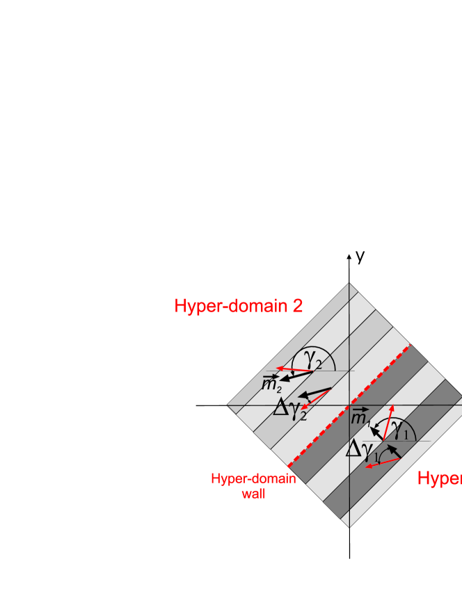
Figure 6: (Color online) Sketch of two hyper-domains separated by the domain wall (red dashed line) along one of the stripe boundary. The magnetization vectors of the hyper-domains are denoted by black arrows tilted by the angles $\gamma_{1,2}$ against the applied field. The red arrows indicate the local magnetization vector tilted randomly and/or periodically by angles $\Delta\gamma_{1,2}$ with respect to the hyper-domain magnetization directions

is the sum of hyper-domain magnetization vectors $\langle{\bm{M}}_{1}\rangle$ and $\langle{\bm{M}}_{2}\rangle$ (see, Fig. 6) weighted in accordance with the percentages $w_{1}$ and $w_{2}=1-w_{1}$ of the sample area they cover. The directions of the vectors of the local magnetization ${\bm{M}}_{1,2}=\langle{\bm{M}}_{1,2}\rangle+\Delta{\bm{M}}_{1,2}$ may vary as a function of the lateral coordinates $x,y$ so that $\Delta{\bm{M}}_{1,2}$ describes local deviations of the local magnetization from their mean values $\langle{\bm{M}}_{1,2}\rangle$ averaged over each of the hyper-domains. Due to the strong anisotropy in the neutron coherency the averaging of the PNR signal, as it was pointed out above, should be performed in two steps. Firstly, the magnetization vectors are averaged over the coherence ellipsoids which are dramatically extended along one axis but still are fitting into any of the hyper-domains. In the particular kinematics the long axis is parallel to the $x-$axis and the coherent averaging results in $\langle{\bm{M}}_{1,2}(x,y)\rangle_{\mathrm{coh}}=\overline{\bm{M}}_{1,2}(y)$. The absolute values $\left|\overline{\bm{M}}_{1,2}(y)\right|$ of these vectors determine the magnetic parts of the optical potentials and reflection amplitudes $R^{\pm}_{1,2}(y)$ for each type of hyper-domain. The amplitudes may still vary as a function of the $y$-coordinate and the equations for SF and NSF reflection intensities require secondly an additional incoherent averaging of the corresponding cross sections along the $y$-direction. Those two types of averaging give access to not only the mean values $\langle{\bm{M}}_{1,2}\rangle=\langle\overline{\bm{M}}_{1,2}(y)\rangle_{\mathrm{inc}}$ in Eq.(5) and, finally, to the net magnetization vector ${\bm{M}}$, but also to the weights $w_{1,2}$. Moreover, the least square routine provides us with quite a few parameters rather characterizing the domain model in great details.

Our model assumes that the projections $M^{x}_{1,2}(x,y)=M_{\mathrm{sat}}\cos\gamma_{1,2}$ and $M^{y}_{1,2}(x,y)=M_{\mathrm{sat}}\sin\gamma_{1,2}$ of the magnetization vectors are determined by the angles $\gamma_{1,2}=\gamma_{1,2}(x,y)=\overline{\gamma}_{1,2}(y)+\Delta\gamma_{1,2}(x,y)$, where $\Delta\gamma_{1,2}(x,y)$ are describing deviations of the angles in directions of the vectors ${\bm{M}}_{1,2}(x,y)$ from that of $\overline{\bm{M}}_{1,2}(y)$. The latter are tilted by $\overline{\gamma}_{1,2}(y)$ against the $x-$axis and are determined by the constrains $\langle\sin\Delta\gamma_{1,2}\rangle_{\mathrm{coh}}=0$ specific for each type of hyper-domains and the $y$-coordinate. The deviation in angles $\Delta\gamma_{1,2}$, either random (ripple domains) and/or periodic (stripes), reduce the absolute values $\left|\overline{\bm{M}}_{1,2}(y)\right|=M_{\mathrm{sat}}c_{1,2}(y)$ by the factors $c_{1,2}(y)=\langle\cos(\Delta\gamma_{1,2})\rangle_{\mathrm{coh}}\leq 1$. These factors generally depend on the $y$-coordinate. However, if the coherence length crosses a large number of stripes and/or ripple domains this dependency is weak and can be neglected in the first approximation so that only two parameters $c_{1}$ and $c_{2}$ characterizing reflection amplitudes are used in the fitting routine. Two other couples of parameters $\overline{C}_{1,2}=\langle\cos\overline{\gamma}_{1,2}(y)\rangle_{\mathrm{inc}}$ and $\overline{S^{2}}_{1,2}=\langle\sin^{2}\overline{\gamma}_{1,2}(y)\rangle_{\mathrm{inc}}$ used to fit the data follow from the incoherent averaging of the PNR cross sections. Such an averaging accounts for fluctuations of the angles $\overline{\gamma}_{1,2}(y)$ determined for different coherence ellipsoids. These fluctuations can be rather developed due to e.g. ripple domains which size is greater than the coherence length in the $y$-direction.

The set of equations for NSF and SF reflectivities used in the data fitting are written as follows toperverg02 ; zabel07 :

$${\mathcal{R}}(P_{i},P_{f}) =w_{1}{\mathcal{R}}_{1}(P_{i},P_{f})+w_{2}{\mathcal{R}}_{2}(P_{i},P_{f})$$

$${\mathcal{R}}_{1,2}(P_{i},P_{f})=\frac{1}{4}\{ [|R^{+}_{1,2}|^{2}+|R^{-}_{1,2}|^{2}][1+P_{i}P_{f}\overline{C^{2}}_{1,2}]$$

$$+ [|R^{+}_{1,2}|^{2}-|R^{-}_{1,2}|^{2}](P_{i}+P_{f})\overline{C}_{1,2}$$ (6)

$$+2\Re(R^{+*}_{1,2}R^{-}_{1,2})P_{i}P_{f}\overline{S^{2}}_{1,2}\},$$

where $P_{i}=\pm|P_{i}|$, $P_{i}=\pm|P_{i}|$ with $|P_{i}|\leq 1$ and $|P_{i}|\leq 1$ are efficiencies of the polarizer and analyzer, respectively. The complex reflection amplitudes $R^{\pm}_{1,2}=R(\pm c_{1,2})$ are determined for two parameters $c_{1}$ and $c_{2}$.

At each value of applied field the best fit of all 4 measured reflection curves was obtained by varying 7 essential parameters: $c_{1,2}$, $\overline{C}_{1,2}$, $\overline{S^{2}}_{1,2}=1-\overline{C^{2}}_{1,2}$ and $w_{2}=1-w_{1}$ while keeping all others found from the fit at saturation where $c_{1,2}=1$, $\overline{C}_{1,2}=1$, $\overline{S^{2}}_{1,2}=0$ and $w_{1}=1$. The quality of the fit is illustrated in Fig. 4, while the results are collected into Fig. 7, where the field variation of the parameters is presented.

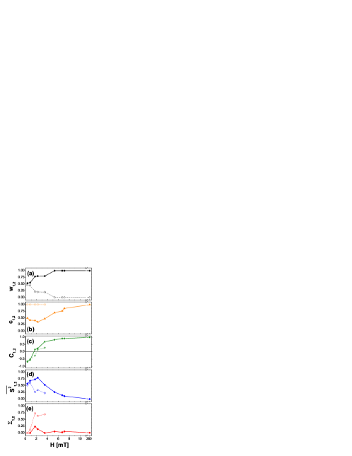
Figure 7: (Color online) Results of fits to the PNR data with respect to the two hyper-domains and as function of the magnetic field. (a) Fraction $w_{1}$ of hyper-domain 1, (b) reduction factor $c_{1}=\langle\cos(\Delta\gamma_{1})\rangle_{\mathrm{coh}}$, (c) parameters $\overline{C}_{1,2}=\langle\cos\overline{\gamma}_{1,2}(y)\rangle_{\mathrm{inc}}$, (d) $\overline{S^{2}}_{1,2}=\langle\sin^{2}\overline{\gamma}_{1,2}(y)\rangle_{\mathrm{inc}}$, and (e) dispersion $\Sigma_{1,2}=\overline{C^{2}}_{1,2}-\overline{C}_{1,2}^{2}$. The solid symbols represent the results of fits to the PNR of the first hyper-domain and the hollow symbols that of the second hyper-domain. Lines in (b)-(d) represent respective results of the MOKE measurements for comparison. Please note that in (d) $\overline{S^{2}}$ can only be achieved from PNR. Instead, the PNR data are compared to $\overline{S}^{2}$ as calculated from $\overline{S}$ from MOKE. In (e) the lines are guides to the eye.

First of all one can admit that two types (Fig. 7(a)) of hyper-domains, one with reduced (Fig. 7(b)) and the other with saturation magnetization, exist almost all over the range of the hysteresis loop. At low fields $w_{1}\approx w_{2}\approx 0.5$, i.e. the two domains states are equally populated. An increasing field $H$ leads to a two step grow of the fraction $w_{1}(H)$ of hyper-domains with reduced magnetization on the cost of those saturated until $w_{1}=1$ and $w_{2}=0$ is reached just below the second coercive field. The reduction factor $c_{1}(H)$ of magnetization in the first type of hyper-domains plotted in Fig. 7(b) is mostly attributed to the angle between the magnetization vectors in neighboring stripes. It is not a monotonous function of field $H$ and $c_{1}(H)$ has a minimum at $H\approx$ 2.2 mT where this angle has a maximum value. In accordance to Fig. 7(c) the magnetization vectors of both types of hyper-domains rotate towards the magnetic field direction but with a different rate. The magnetization of ”striped” hyper-domains approaches the applied field direction much faster than that of hyper-domains with its magnetization close to saturation. Note that at the two lowest values $H=0.3$ and $H=0.8$ mT the magnetization of both types of domains has a negative projection onto the field direction. At the next measured field $H=1.7$ mT the parameter $\overline{C}_{1}>0$, meaning that the magnetization vector $x$-projection of the unsaturated hyper-domains now is positive. At the same field $\overline{C}_{2}<0$, i.e. the magnetization vectors of the saturated hyper-domains is tilted with respect to the field by angles of $90^{\circ}<\overline{\gamma}_{2}<270^{\circ}$. Further increase of magnetic field pull both magnetization vectors to the field direction.

Eq.(6) contains only $\overline{S^{2}}_{1,2}=\langle\sin^{2}\overline{\gamma}\rangle$ plotted in Fig. 7(d), but not $\langle\sin\overline{\gamma}\rangle^{2}$. Therefore, as already mentioned, with PNR alone we cannot determine the sense of rotation. The missing information is compensated due to the vector-MOKE measurements presented in Fig. 1, while PNR provides access to the dispersions $\Sigma_{1,2}=\overline{C^{2}}_{1,2}-\overline{C}_{1,2}^{2}$, additional physical parameters plotted in Fig. 7(e). These quantities measure a degree of magnetization vector fluctuations in hyper-domains of the same type. Hence, $\Sigma_{1}\ll 1$ all over the range of fields signifying on rather coherent rotation of the magnetization vector in different hyper-domains with reduced magnetization. For the other type of hyper-domains $\Sigma_{2}$, on the contrary, is rather high and reveals non-monotonous behavior. This means that the magnetization vector in different highly saturated hyper-domains is tilted by quite different angles $\overline{\gamma}_{2}$ indicating the fact that there actually exist more types of hyper-domains with nearly saturated magnetization. Such hyper-domains can be distinguished on some of the KM images McCord , but unfortunately, the quality of our present PNR data seems not allowing to introduce more parameters for their identification.

However, our data, e.g. presented in Fig. 5 are well sufficient to infer the microscopic magnetic structure of hyper-domains and prove the model sketched in Fig. 6. Indeed, using parameters found from the fit of specular reflectivities we can identify the reference state of the system perturbed by periodic (stripe domains) and random (ripple domains) deviations of magnetization from its mean value in each type of hyper domains. Comparing intensity along the diffraction lines in the maps in Fig. 5 with specularly reflected intensity we determined the angles between magnetization directions in stripe domains and direction of magnetization of hyper-domain. For instance, at 6.7 mT it was found that $\overline{\beta}_{1}=30^{\circ}$ and $\overline{\beta}_{2}=0^{\circ}$, i.e. the angle between magnetization directions in neighboring stripes amounts $30^{\circ}$. The tilt angles was, actually, found by taking into account, that the intensity of the Bragg lines is reduced due to ripple domains. They cause magnetization fluctuations reducing the magnetic scattering contrast between stripe domains and simultaneously creating diffuse scattering seen in Fig. 5. The intensity of diffuse scattering allows us to quantify the amplitude of those fluctuations. In the case of $H=$6.7 mT ripple domains reduce stripe magnetization for about 10% with respect to saturation. However, fluctuations are not absolutely random but correlated over a few of neighboring stripes as is found from the extension of diffuse scattering in Fig. 5. The role of correlated magnetization fluctuations Theis-Broehl05 is not yet very clear, but they certainly strongly influence a formation of hyper-domains in the alternating EB systems and hence a scenario of the re-magnetization process.

V Summary

In summary, by using vector-MOKE magnetometry, Kerr microscopy and polarized neutron reflectometry we studied the field induced evolution of the magnetization distribution of a periodic pattern of alternating exchange bias stripes when applying the magnetic field at an angle of 45^∘ in order to avoid the instability with respect to the tilt of magnetization found for the easy axis configuration Theis-Broehl_PRB2006 . The data show that the re-magnetization process proceeds through different stages which are qualitatively described by comprehensive analysis of specular and off-specular PNR data. Beside the formation of stripe-domains with alternated in-plane magnetization at small fields small ripple domains and two types large hyper-domains develop comprising a number of stripes. We developed a microscopic picture of the magnetic structure based on the results of our polarized neutron studies which to some extent could be verified via Kerr microscopy.

- (1) J. Nogus, I. K. Schuller, J. Magn. Magn. Mater. 192, 203 (1999).
- (2) A. Berkowitz A., K. Takano K., J. Magn. Magn. Mater. 200, 552 (1999).
- (3) R. L. Stamps, J. Phys. D 23, R247 (2000).
- (4) M. Kiwi M., J. Magn. Magn. Mater. 234, 584 (2001).
- (5) J. Nogués, J. Sorta, V. Langlais, V. Skumryev, S. Suriñach, J.S. Muñoz, M.D. Baró, Physics Reports 422, 65 (2005).
- (6) A. Moser, K. Takano, D.T. Margulies, M. Albrecht, Y. Sonobe, Y. Ikeda, S. Sun, and E. E. Fullerton, J. Phys. D 35, R157 (2002).
- (7) D. Suess, M. Kirschner, T. Schrefl, J. Fidler, R.L. Stamps, and J.-V. Kim, Phys. Rev. B 58, 97 (1998).
- (8) T.M. Hong, Phys. Rev. B 67, 9054419 (2003).
- (9) H. Ohldag, A. Scholl, F. Nolting, E. Arenholz, S. Maat, A.T. Young, M. Carey, and J. Stöhr, Phys. Rev. Lett. 91, 017203 (2003).
- (10) J. Schmalhorst, V. Höink, G. Reiss, D. Engel, D. Junk, A. Schindler, A. Ehresmann, and H. Schmoranzer J. Appl. Phys. 94, 5556 (2003).
- (11) D. Engel, A. Kronenberger, M. Jung, H. Schmoranzer, A. Ehresmann, A. Paetzold, and K. R ll, J. Magn. Magn. Mater. 263, 275 (2003).
- (12) A. Ehresmann, Recent Res. Dev. Phys. 7, 401 (2004).
- (13) K. Theis-Bröhl, M. Wolff, A. Westphalen , H. Zabel, J. McCord, V. Höink, J. Schmalhorst, G. Reiss, T. Weis, D. Engel, A. Ehresmann, U. Rücker, B.P. Toperverg Phys. Rev. B 73 174408 (2006).
- (14) A. P. Malozemoff, Phys. Rev. B, 35, 3679 (1987).
- (15) A. P. Malozemoff, Phys. Rev. B, 37, 7673 (1988).
- (16) V. Deriglazov et al. (to be published).
- (17) J. McCord, R. Schäfer, K. Theis-Bröhl, H. Zabel, J. Schmalhorst, V. Höink, H. Brückl, T. Weiss, D. Engel, and A. Ehresmann, J. Appl. Phys. 97, 10K102 (2005).
- (18) T. Schmitte, K. Theis-Bröhl, V. Leiner, H. Zabel, S. Kirsch, and A. Carl, J. Phys.: Condens. Matter 14, 7525 (2002).
- (19) A. Hubert and R. Schäfer, Magnetic domains (Springer, Heidelberg, 1998).
- (20) K. Theis-Bröhl, T. Schmitte, V. Leiner, H. Zabel, K. Rott, H. Brückl, and J. McCord, Phys. Rev. B 67, 184415 (2003).
- (21) B. P. Toperverg, G. P. Felcher, V. V. Metlushko, V. Leiner, R. Siebrecht, O. Nikonov, Physica B283, 149 (2000).
- (22) B. P. Toperverg, A. Rühm, W. Donner, H. Dosch, Physica B, 267-268, 98, (1999).
- (23) B. P. Toperverg, In Polarized Neutron Scattering, by Th. Brückel and W. Schweika (Eds.), Series Matter and Materials, v.12, Jülich, v.12, p.274 (2002).
- (24) H. Zabel, K. Theis-Bröhl, B.P. Toperverg, Polarized neutron reflectivity and scattering of magnetic nanostructures and spintronic materials, In Handbook of Magnetism and Advanced Magnetic Materials by H. Kronmüller/ S. Parkin (Eds.), Wiley p. 1237 (2007).
- (25) K. Theis-Bröhl, B. P. Toperverg, V. Leiner, A. Westphalen, H. Zabel J. McCord, H. Rott, H. Brückl, Phys. Rev. B 71, 020403(R) 2005.