Spin-charge separation in transport through Luttinger liquid rings

Abstract

We investigate how the different velocities characterizing the low-energy spectral properties and the low-temperature thermodynamics of one-dimensional correlated electron systems (Luttinger liquids) affect the transport properties of ring-like conductors. The Luttinger liquid ring is coupled to two noninteracting leads and pierced by a magnetic flux. We study the flux dependence of the linear conductance. It shows a dip structure which is governed by the interaction dependent velocities. Our work extends an earlier study which was restricted to rather specific choices of the interaction parameters. We show that for generic repulsive two-particle interactions the number of dips can be estimated from the ratio of the charge current velocity and the spin velocity. In addition, we clarify the range of validity of the central approximation underlying the earlier study.

I Introduction

In the presence of a two-particle interaction the low-temperature thermodynamics and the low-energy spectral properties of a wide class of one-dimensional (1d) electron systems is described by the Luttinger liquid (LL) phenomenology.Schoenhammer05 One of the characterizing properties of a LL is the complete separation of the fundamental collective spin and charge excitations. In the low-energy limit and for a fixed number of left and right moving electrons the Hamiltonian can be written as the sum of two terms describing free bosons for the spin and charge degrees of freedom, both having a linear dispersion with velocities $v_{s}$ and $v_{c}$. Furthermore, in 1d the bosonic degrees of freedom span the entire low-energy Hilbert space at fixed particle number. This has to be contrasted to the collective spin and charge excitations of higher dimensional Fermi liquids which only give a certain part of the spectrum. In many theoretical studies the effect of spin-charge separation was discussedSchoenhammer05 ; Argentinier ; VM1 ; Voit ; Uli and there have been several attempts to find experimental indications for it.experiments

The low-energy physics of a LL is parameterized by four (in general) independent and interaction dependent fundamental velocities $v_{N,c}$, $v_{N,s}$, $v_{J,c}$, and $v_{J,s}$. The first two are relevant when the total charge or spin are changed, while the later two are the velocities characterizing the charge and spin current. From these, $v_{s}$ and $v_{c}$ can be computed asSchoenhammer05

$$v_{c/s}=\sqrt{v_{N,c/s}\;v_{J,c/s}}\;.$$ (1)

Here we are interested in the role of spin-charge separation or more generally in the role of the different interaction dependent velocities on transport through LLs. There is no specific effect on the linear conductance $G$ of a linear LL wire connected to a Fermi liquid source and drain. A different situation occurs if a closed LL ring coupled via tunnel barriers to two noninteracting leads is considered. This geometry allows for interference and an additional parameter can be added to the problem, namely a magnetic flux $\phi$ piercing the ring. The linear conductance then becomes a periodic function of $\phi$ with a periodicity of one flux quantum $\phi_{0}$. We here chose units such that $\phi_{0}=2\pi$.

In Ref. Jagla, it was argued that for $v_{c}/v_{s}=q/p$, with $q$ and $p$ being “small” odd numbers, $G(\phi)$ shows characteristic dips whose number for $\phi\in[0,2\pi]$ is given by $qv_{F}/v_{c}=pv_{F}/v_{s}$, with $v_{F}$ being the noninteracting Fermi velocity. The appearance of such dips might thus be interpreted as an indication of spin-charge separation. Restricting the ratio of the charge and spin velocities to such cases, however requires rather specific interaction parameters which will be hard to realize in experimental systems. The authors study a continuum model, the Tomonaga-Luttinger model (TLM). The central approximation of this work—which can be applied for the above given ratio of $v_{c}$ and $v_{s}$—is related to the idea that an electron can pass the ring only if the charge and spin can “recombine” at the right (and left) contact (for details see below). A dip structure of $G(\phi)$ was also obtained for a small ring described by a lattice model with strong local Coulomb interaction, the 1d $t-J$ model.Hallberg

We here reinvestigate the zero temperature transport through a LL ring described by the TLM. We do not rely on the above mentioned approximation of Ref. Jagla, and present results for arbitrary repulsive interactions, thus being closer to situations which can be realized in experimental setups. This extends the earlier study and clarifies the range of applicability of the central approximation underlying that work. More precisely, we find that the approximation of Ref. Jagla, leads to qualitatively correct results only if the smaller of the two numbers, say $p$,footnote is either $1$, $3$ or $5$, with the refinement that for $p=3$ or $5$ the other number $q$ may not exceed $7$. Furthermore, the important role of the charge current velocity $v_{J,c}$ as a factor accompanying the magnetic flux in all relevant formulas was largely overlooked so far. While, according to the approximation made in Ref. Jagla, , the transmission probability exhibits $p\,v_{F}/v_{s}=q\,v_{F}/v_{c}$ dips over one period of the magnetic flux, we find that the expression $v_{J,c}/v_{s}$ gives a much better estimate on the number of dips in almost all cases. It is thus the charge current velocity and not the velocity $v_{c}$ of the bosonic modes which is of relevance for the dip structure of $G(\phi)$. We also clarify how the two expressions for the number of dips and their respective partial viabilities are related.

Transport through LL rings weakly coupled to noninteracting leads was also studied in Refs. Kinaret, and Mikhail, although with a focus different to ours.

The rest of this paper is organized as follows. To set the stage we introduce the TLM and our way to compute the linear conductance in Sec. II. The latter involves the one-particle Green function of the TLM which we also discuss in this section. In Sec. III we describe the approximation of Ref. Jagla, and the corresponding results for the flux dependence of the linear conductance. Our results for $G(\phi)$ are discussed in Sec. IV and compared to the earlier findings of Ref. Jagla, . We also comment on the relation to the numerical study Ref. Hallberg, . We conclude with a summary in Sec. V.

II Model and methods

II.1 The Tomonaga-Luttinger model

The low-energy physics of 1d correlated metals is governed by long-range effective forces. Consequently, relevant wave numbers are from relatively narrow momentum intervals close to the Fermi momenta $\pm k_{F}$.Schoenhammer05 It is then natural to linearize the free dispersion relation around the two Fermi momenta. The electrons are separated into two classes, namely into right- and left-moving fermions, respectively. The Hamiltonian then reads (in standard second quantized notation)

$$H= H_{0}+H_{\rm{int}},$$ (2)

$$H_{0}= {\sum_{k}}^{\prime}\sum_{\alpha,\sigma}\alpha v_{F}(k-\alpha k_{F})c^{\dagger}_{k,\alpha,\sigma}c_{k,\alpha,\sigma},$$

$$H_{\rm{int}}= \frac{1}{2L}{\sum_{k,k^{\prime},q}}^{\prime}\sum_{\sigma,\sigma^{\prime}}\sum_{\alpha,\alpha^{\prime}}\tilde{v}^{\sigma,\sigma^{\prime}}_{\alpha,\alpha^{\prime}}(q)c^{\dagger}_{k+q,\alpha,\sigma}c^{\dagger}_{k^{\prime}-q,\alpha^{\prime},\sigma^{\prime}}$$

$$\times c_{k^{\prime},\alpha^{\prime},\sigma^{\prime}}c_{k,\alpha,\sigma}\;,$$

with $\alpha=\pm$ labeling the two branches and $\sigma$ the spin direction. The prime at the momentum sums indicates that the momenta are restricted to a range $2\Lambda$ around the two Fermi points, with the momentum cutoff $\Lambda>0$. Since the electrons move in a finite system of length $L$ with periodic boundary conditions, the $k$-sum is over discrete values $k_{n}=\frac{2\pi}{L}n$, $n\in{\mathbb{Z}}$. The elements of the interaction matrix are conveniently classified according to the so-called g-ology convention.solyom For the TLM the following couplings are relevant:

$$\tilde{v}^{\sigma,\sigma}_{\alpha,\alpha}(q)=g_{4,\parallel}(q)\;,\;\;\;\;\tilde{v}^{\sigma,-\sigma}_{\alpha,\alpha}(q)=g_{4,\perp}(q)\;,$$

$$\tilde{v}^{\sigma,\sigma}_{\alpha,-\alpha}(q)=g_{2,\parallel}(q)\;,\;\;\;\;\tilde{v}^{\sigma,-\sigma}_{\alpha,-\alpha}(q)=g_{2,\perp}(q)\;.$$ (3)

The $g_{4}$-processes correspond to intra-branch and the $g_{2}$-processes to inter-branch scattering. The $\parallel$ - index indicates processes involving two electrons of parallel spin orientation while $\perp$ stands for scattering of electrons with opposite spin.

After normal ordering the operators with respect to the ground state and sending the momentum cutoff $\Lambda$ to $\infty$ the model can be solved exactly using bosonization, that is the introduction of bosonic creation and annihilation operators.Schoenhammer05 ; Herbert The first step towards bosonization is to consider the density operators ($q\neq 0$)

$$\rho_{q,\alpha,\sigma}=\sum_{k}c^{\dagger}_{k,\alpha,\sigma}c_{k+q,\alpha,\sigma}\;.$$ (4)

Operators $b^{\dagger}_{q,\sigma}$ and $b_{q,\sigma}$ obeying bosonic commutation relations are obtained defining

$$b_{q,\sigma}=\sqrt{\frac{2\pi}{|q|L}}\begin{cases}\rho_{q,+,\sigma}&q>0\\ \rho_{q,-,\sigma}&q<0\end{cases}\;.$$ (5)

These operators as well as the different couplings $g_{2}$ and $g_{4}$ may be mapped onto new ones which are no longer associated with the two spin directions but with collective charge and spin excitations of the system, respectively ($\nu=2,4$)

$$b_{q,c}\equiv\frac{1}{\sqrt{2}}(b_{q,\uparrow}+b_{q,\downarrow})\;,$$

$$b_{q,s}\equiv\frac{1}{\sqrt{2}}(b_{q,\uparrow}-b_{q,\downarrow})\;,$$ (6)

$$g_{\nu,c}(q)\equiv g_{\nu,\parallel}+g_{\nu,\perp}\;,$$

$$g_{\nu,s}(q)\equiv g_{\nu,\parallel}-g_{\nu,\perp}\;.$$ (7)

We define excess particle number operators ${\mathcal{N}}_{\alpha,\sigma}$ with respect to the ground state (normal ordering). Spin and charge operators for a fixed branch index are obtained as the linear combinations

$$\mathcal{N}_{\alpha,c/s}=\frac{1}{\sqrt{2}}\left(\mathcal{N}_{\alpha,\uparrow}\pm\mathcal{N}_{\alpha,\downarrow}\right)\;,$$ (8)

charge and spin current operators as ($a=c/s$)

$$\mathcal{J}_{a}=\mathcal{N}_{+,a}-\mathcal{N}_{-,a}$$ (9)

and the total particle number and spin operators as

$$\mathcal{N}_{a}=\mathcal{N}_{+,a}+\mathcal{N}_{-,a}\;.$$ (10)

In terms of these newly defined operators and couplings, the Hamiltonian splits up into two commuting parts

$$H^{\rm TL}=H^{\rm TL}_{c}+H^{\rm TL}_{s}$$ (11)

with

$$H^{\rm TL}_{a} = \sum_{k>0}\left\{k\Big{[}v_{F}+\frac{g_{4,a}(k)}{2\pi}\Big{]}\left(b^{\dagger}_{k,a}b_{k,a}+b^{\dagger}_{-k,a}b_{-k,a}\right)\right.$$ (12)

$$\left.+k\frac{g_{2,a}(k)}{2\pi}\left(b^{\dagger}_{k,a}b^{\dagger}_{-k,a}+b_{-k,a}b_{k,a}\right)\right\}$$

$$+\frac{\pi}{2L}\left(v_{J,a}\mathcal{J}_{a}^{2}+v_{N,a}\mathcal{N}_{a}^{2}\right)\;.$$

The velocities $v_{J,a}$ and $v_{N,a}$ are defined in terms of the couplings as

$$v_{N/J,a}=v_{F}+\frac{g_{4,a}(0)\pm g_{2,a}(0)}{2\pi}\;.$$ (13)

The part of $H^{\rm TL}_{a}$ involving bosonic operators can be diagonalized by a Bogoliubov transformationSchoenhammer05 leading to a Hamiltonian of free and uncoupled bosons with dispersion $\omega_{a}(k)=v_{a}(k)|k|$ and velocities

$$v_{a}(k) =v_{F}\left(1+\frac{g_{4,a}(k)+g_{2,a}(k)}{2\pi v_{F}}\right)^{1/2}$$ (14)

$$\times\left(1+\frac{g_{4,a}(k)-g_{2,a}(k)}{2\pi v_{F}}\right)^{1/2}\;.$$

In the limit $k\to 0$ this leads to the charge and spin velocities defined in Eq. (1).

In the low-energy limit the details of the momentum dependence of the couplings are generically irrelevant as long as the $g_{\nu,\parallel/\perp}(k)$ are slowly varying functions close to $k=0$ (for an exception see Ref. VM3, ). Without loss of generality we thus assume that

$$g_{\nu,\parallel/\perp}(k)=g_{\nu,\parallel/\perp}\,\Theta(k_{c}-|k|)\;,$$ (15)

with a cutoff $k_{c}=2\pi n_{c}/L\ll k_{F}$ of the momentum transfer. Therefore the velocities $v_{a}$ are independent of $k$ for all $k\leq k_{c}$. With this choice a closed expression for the retarded one-particle Green function $\tilde{\mathcal{G}}^{R}(x,\omega)$ of the homogeneous TLM can be given, which enters the approximate expression for the conductance through the ring used here. To obtain the Green function we follow the procedure introduced in Ref. VM4, (see below).

II.2 The Luttinger liquid ring with magnetic flux

We now consider a ring of finite length $L$ described by the TLM that is pierced by a magnetic flux $\phi$. The term $H_{{\mathcal{J}}}^{c}=\pi v_{J,c}{\mathcal{J}}_{c}^{2}/(2L)$ in the Hamiltonian Eq. (12) must then be replaced byLoss ; PeterS ; VM2

$$H_{\mathcal{J}}^{c} = \frac{v_{J,c}\pi}{2L}\left({\mathcal{J}}_{c}-\sqrt{2}\,\frac{\phi}{\pi}\right)^{2}$$ (16)

$$= \frac{v_{J,c}\pi}{2L}\left({\mathcal{J}}_{c}^{2}-2\,\sqrt{2}\,{\mathcal{J}}_{c}\,\frac{\phi}{\pi}+2\,\left[\frac{\phi}{\pi}\right]^{2}\right)$$

It is important to note that the characteristic velocity appearing in the flux dependent part of the Hamiltonian is the current velocity $v_{J,c}$. This can easily be seen as follows. For a system with an equal number of left and right moving electrons $\left<{\mathcal{J}}_{c}\right>=0$ and the last term in Eq. (16) determines the ground state persistent current $I=-dE_{0}(\phi)/d\phi$, with $E_{0}$ being the ground state energy. It was shown numericallyPeterS ; VM2 for lattice models that the velocity appearing in the persistent current is the charge current velocity $v_{J,c}$. In Ref. Jagla, mostly $v_{F}$ was used instead of $v_{J,c}$. Only for Galilean invariant systems both velocities are equal,Schick which indicates that the authors of Ref. Jagla, had such systems in mind without mentioning it explicitly.

We later need to compute the one-particle Green function of the isolated LL ring. The term linear in the flux of Eq. (16) affects this correlation function. Using Eqs. (9) and (8) the $\phi$-linear term can be written as

$$-\frac{v_{J,c}\pi}{2L}\,2\,\sqrt{2}\,{\mathcal{J}}_{c}\,\frac{\phi}{\pi}=-\frac{v_{J,c}\phi}{L}$$

$$\times(\mathcal{N}_{+,\uparrow}+\mathcal{N}_{+,\downarrow}-\mathcal{N}_{-,\uparrow}-\mathcal{N}_{-,\downarrow})$$ (17)

and the prefactor of the operator part can be understood as an $\alpha$-dependent correction of the chemical potential $\delta\mu_{\alpha}$. It thus appears as a phase factor $\exp{(-i\,\delta\mu_{\alpha}\,t)}$ in the Green function [see Eq. (20)].

II.3 The conductance of the Luttinger liquid ring

Next, the finite size LL ring is coupled via tunnel barriers with hopping matrix elements $t^{\prime}$ to left and right leads at positions $x=0$ and $x=L/2$. For simplicity we assume equal left and right tunnel barriers. To be specific both leads are described as 1d tight-binding chains with hopping matrix element $\tau$, but we expect our results to be independent of the precise form of the band structure of the reservoirs.

For noninteracting electrons the transmission probability per spin direction through the ring can be expressed in terms of the spin-independent retarded one-particle Green function $\tilde{\mathcal{G}}^{R}(x,\omega)$ of the isolated ring at position $0$ and $L/2$. It is given byJagla (for a simple derivation of this formula see Sec. III of Ref. Tilman, )

$$T(\omega)=\frac{4\tau^{2}\sin^{2}k\left|Lt^{\prime 2}\tilde{\mathcal{G}}^{R}(L/2,\omega)\right|^{2}}{\left|[\omega-Lt^{\prime 2}\tilde{\mathcal{G}}^{R}(0,\omega)+\tau e^{ik}]^{2}-\left|Lt^{\prime 2}\tilde{\mathcal{G}}^{R}(L/2,\omega)\right|^{2}\right|^{2}}\;.$$ (18)

The zero temperature conductance, on which we focus, follows by setting $\omega=0$, that is the energy equal to the chemical potential, and multiplying $T$ by $2e^{2}/h$. In Refs. Jagla, and Hallberg, it was argued that this expression can also be used in the presence of interactions in the ring provided $t^{\prime}$ is sufficiently small and the Kondo effect does not play a role. The latter holds in parameter regimes with an average number of electrons on the ring which is even. That the general features of the conductance through an interacting ring which is not in the Kondo regime are indeed captured to some extent by the approximate Eq. (18) was shown in Ref. Simon, using a functional renormalization group approach which can be applied for sufficiently weak interactions but is nonperturbative in the coupling to the leads. Thus we will here also rely on Eq. (18).

II.4 The Green function of the $g_{4}$-model

In a first step we study the so-called $g_{4}$-model in which all inter-branch scattering processes are set to zero. We decompose the retarded Green function as

$$i\,{\mathcal{G}}^{R}(x,t)=\theta(t)\sum_{\alpha=\pm}\left[i\,{\mathcal{G}}_{\alpha}^{>}(x,t)+i\,{\mathcal{G}}_{\alpha}^{<}(x,t)\right]\;,$$ (19)

with the greater ${\mathcal{G}}_{\alpha}^{>}$ and lesser ${\mathcal{G}}_{\alpha}^{<}$ Green functions of right ($\alpha=+$) and left ($\alpha=-$) moving electrons. Using bosonization of the field operatorSchoenhammer05 ; Herbert for the box-shaped potential Eq. (15), these Green functions are given byVM4

$$i\,\mathcal{G}_{\alpha}^{>/<}(x,t)=i\,e^{i\alpha\phi v_{J,c}t/L}\mathcal{G}_{\alpha}^{>/<,0}(x,t)e^{F^{>/<}_{\alpha}(x,t)}$$ (20)

where

$$F^{>/<}_{\alpha}(x,t)=\sum_{n=1}^{n_{c}}\frac{1}{n}\left[\frac{1}{2}e^{\pm i\,\frac{2\pi}{L}n(\alpha x-v_{c}t)}\right.$$

$$\left.+\frac{1}{2}e^{\pm i\,\frac{2\pi}{L}n(\alpha x-v_{s}t)}-e^{\pm i\,\frac{2\pi}{L}n(\alpha x-v_{F}t)}\right]\;.$$ (21)

The noninteracting Green functions read

$$i\,\mathcal{G}_{\alpha}^{>,0}(x,t) = \frac{1}{L}e^{i\alpha k_{F}x}e^{i\,\frac{2\pi}{L}\left(\alpha x-v_{F}t\right)}$$

$$\times\left[1-e^{i\,\frac{2\pi}{L}\left(\alpha x-v_{F}t+i0\right)}\right]^{-1}\;,$$

$$i\,\mathcal{G}_{\alpha}^{<,0}(x,t) = \frac{1}{L}e^{i\alpha k_{F}x}$$ (22)

$$\times\left[1-e^{-i\,\frac{2\pi}{L}\left(\alpha x-v_{F}t-i0\right)}\right]^{-1}\;.$$

The second exponential factor in the equation for $\mathcal{G}_{\alpha}^{>,0}$ appears due to the choice of $\pm k_{F}=\pm 2\pi n_{F}/L$ corresponding to the last occupied level. For $L\to\infty$ it becomes unity, but is relevant in our case as we study rings of finite length. As discussed in Ref. VM4, the Fourier transform of the greater Green function can be computed iteratively as

$$\tilde{\mathcal{G}}^{>}_{\alpha}(x,\omega)=\frac{e^{i\alpha(k_{F}+\frac{2\pi}{L})x}}{L}\sum_{m=0}^{\infty}\sum_{l=0}^{m}\sum_{j=0}^{m-l}$$

$$\frac{a_{m-l-j}^{(n_{c})}b_{l}^{(n_{c})}b_{j}^{(n_{c})}e^{i\alpha\frac{2\pi}{L}mx}}{\omega+\alpha\phi v_{J,c}/L-\frac{2\pi}{L}\big{[}(m-l-j+1)v_{F}+lv_{c}+jv_{s}\big{]}+i0}\;,$$ (23)

with

$$a_{lm+n}^{(m)} = \sum_{j=0}^{l}\frac{(-1/m)^{j}}{j!}a_{m(l-j)+n}^{(m-1)}\;,$$

$$b_{lm+n}^{(m)} = \sum_{j=0}^{l}\frac{(1/2m)^{j}}{j!}b_{m(l-j)+n}^{(m-1)}$$ (24)

and initial values

$$a_{m}^{(1)} = \sum_{j=0}^{m}\frac{(-1/j)}{j!}\;,$$

$$b_{m}^{(1)} = \frac{(1/2)^{m}}{m!}\;.$$ (25)

Similarly, the lesser Green function reads

$$\tilde{\mathcal{G}}^{<}_{\alpha}(x,\omega)=\frac{e^{i\alpha k_{F}x}}{L}\sum_{m=0}^{\infty}\sum_{l=0}^{m}\sum_{j=0}^{m-l}$$

$$\frac{a_{m-l-j}^{(n_{c})}b_{l}^{(n_{c})}b_{j}^{(n_{c})}e^{-i\alpha\frac{2\pi}{L}mx}}{\omega+\alpha\phi v_{J,c}/L+\frac{2\pi}{L}\big{[}(m-l-j)v_{F}+lv_{c}+jv_{s}\big{]}+i0}\;.$$ (26)

It is easy to see that for $|k\pm k_{F}|<q_{c}$ the one-particle spectral function as a function of energy obtained by taking the imaginary part of the momentum Fourier transform of Eqs. (23) and (26) has support only between $\pm v_{s}|k\pm k_{F}|$ and $\pm v_{c}|k\pm k_{F}|$.VM4 In the thermodynamic limit the spectral weight shows a square-root singularity at the two edges. The corresponding Green functions (for $|x|,v_{F}|t|\gg 1/q_{c}$) in the $(x,t)$-plane are given by

$$i\,{\mathcal{G}}^{>}_{\alpha}(x,t)=\frac{1}{L}e^{i\alpha k_{F}x}e^{i\alpha\phi v_{J,c}t/L}e^{i\,\frac{2\pi}{L}\left(\alpha x-v_{F}t\right)}$$

$$\times\left[1-e^{i\frac{2\pi}{L}(\alpha x-v_{c}t+i0)}\right]^{-1/2}\left[1-e^{i\frac{2\pi}{L}(\alpha x-v_{s}t+i0)}\right]^{-1/2}\;,$$

$$i\,{\mathcal{G}}^{<}_{\alpha}(x,t)=\frac{1}{L}e^{i\alpha k_{F}x}e^{i\alpha\phi v_{J,c}t/L}$$

$$\times\left[1-e^{-i\frac{2\pi}{L}(\alpha x-v_{c}t-i0)}\right]^{-1/2}\left[1-e^{-i\frac{2\pi}{L}(\alpha x-v_{s}t-i0)}\right]^{-1/2}\;.$$ (27)

Power-laws with anomalous (interaction dependent) exponents only appear if also the $g_{2}$ terms are kept.Schoenhammer05 Below we return to Eq. (27) when discussing the results of Ref. Jagla, . As the anomalous contributions to the propagator were neglected in this work, it is the $g_{4}$-model which was effectively studied.

From Eqs. (13) and (14) it follows that in the $g_{4}$-model the charge current velocity $v_{J,c}$ and the charge velocity $v_{c}$ are equal.

II.5 Green function of the full model

Also for the full model with intra- and inter-branch scattering processes a closed iterative expression for the Green function can be given if a box-shaped two-particle interaction is assumed. Now, the anomalous dimensions $\gamma_{s}=s_{s}^{2}$ and $\gamma_{c}=s_{c}^{2}$ appear. The variables $s_{a}$ are defined by $s_{a}(q)=\sinh\Theta_{q,a}$ at $q=0$ and the angle $\Theta_{q,a}$ characterizes via

$$\beta_{q,a}=b_{q,a}\cosh\Theta_{q,a}-b_{-q,a}^{\dagger}\sinh\Theta_{q,a}$$ (28)

the canonical transformation to new annihilation (creation) operators $\beta_{q,a}^{(\dagger)}$ by means of which the bosonized TL-Hamiltonian is diagonalized. The angle $\Theta_{q,a}$ depends on the couplings according to the formula

$$\tanh(2\Theta_{q,a}) = -\Big{[}\frac{g_{2,\parallel}(q)\pm g_{2,\perp}(q)}{2\pi v_{F}}\Big{]}$$ (29)

$$\times\Big{[}1+\frac{g_{4,\parallel}(q)\pm g_{4,\perp}(q)}{2\pi v_{F}}\Big{]}^{-1}$$

where the “$+$”-signs are relevant for the charge angle $\Theta_{q,c}$ and the “$-$”signs for the spin angle $\Theta_{q,s}$. The function $F^{>/<}_{\alpha}(x,t)$ in Eq. (20) now reads

$$F^{>/<}_{\alpha} (x,t)=\sum_{n=1}^{n_{c}}\frac{1}{n}\Big{[}\frac{1+s_{c}^{2}}{2}e^{\pm i\frac{2\pi}{L}n(\alpha x-v_{c}t)}$$

$$+\frac{s_{c}^{2}}{2}e^{\mp i\frac{2\pi}{L}n(\alpha x+v_{c}t)}+\frac{1+s_{s}^{2}}{2}e^{\pm i\frac{2\pi}{L}n(\alpha x-v_{s}t)}$$ (30)

$$+\frac{s_{s}^{2}}{2}e^{\mp i\frac{2\pi}{L}n(\alpha x+v_{s}t)}-e^{\pm i\frac{2\pi}{L}n(\alpha x-v_{F}t)}-s_{c}^{2}-s_{s}^{2}\Big{]}.$$

Because of the assumed box-like shape of the two-particle interaction (in momentum space) the $s_{a}(q)$ are independent of $q=q_{n}=2\pi n/L$ for all $n\leq n_{c}$.

We again introduce recursively defined coefficients. The $a_{m}^{(n_{c})}$ are given as in Eq. (24) and coefficients $b_{m,a}^{(n_{c})}$ as well as $c_{m,a}^{(n_{c})}$ are computed according to the formulas

$$\begin{split}b_{lm+i,a}^{(m)}=\sum_{j=0}^{l}\frac{\left([1+\gamma_{a}]/[2m]\right)^{j}}{j!}b_{m(l-j)+i,a}^{(m-1)}\;,\\ c_{lm+i,a}^{(m)}=\sum_{j=0}^{l}\frac{\left(\gamma_{a}/[2m]\right)^{j}}{j!}c_{m(l-j)+i,a}^{(m-1)}\end{split}$$ (31)

with initial conditions

$$\begin{split}b_{m,a}^{(1)}=\frac{\left([1+\gamma_{a}]/2\right)^{m}}{m!},\\ c_{m,a}^{(1)}=\frac{\left(\gamma_{a}/2\right)^{m}}{m!}.\end{split}$$ (32)

In analogy to Eq. (23) one can bring the greater and lesser Green functions into the form

$$\begin{split}&\tilde{{\mathcal{G}}}^{>}_{\alpha}(x,\omega)=A^{-\gamma_{c}-\gamma_{s}}\frac{e^{i\alpha(k_{F}+\frac{2\pi}{L})x}}{L}\\ &\sum_{m=0}^{\infty}\sum_{l=0}^{m}\sum_{j=0}^{l}\sum_{p=0}^{m-l}\sum_{q=0}^{p}a_{m-l-p}^{(n_{c})}b_{l-j,c}^{(n_{c})}c_{j,c}^{(n_{c})}b_{p-q,s}^{(n_{c})}c_{q,s}^{(n_{c})}\\ &\frac{e^{i\alpha\frac{2\pi}{L}(m-2j-2q)x}}{\omega+\alpha\phi v_{J,c}/L-\frac{2\pi}{L}\left(\big{[}(m+1-l-p)v_{F}-lv_{c}-pv_{s}\big{]}\right)+i0}\end{split}$$ (33)

and

$$\begin{split}&\tilde{\mathcal{G}}^{<}_{\alpha}(x,\omega)=A^{-\gamma_{c}-\gamma_{s}}\frac{e^{i\alpha k_{F}x}}{L}\\ &\sum_{m=0}^{\infty}\sum_{l=0}^{m}\sum_{j=0}^{l}\sum_{p=0}^{m-l}\sum_{q=0}^{p}a_{m-l-p}^{(n_{c})}b_{l-j,c}^{(n_{c})}c_{j,c}^{(n_{c})}b_{p-q,s}^{(n_{c})}c_{q,s}^{(n_{c})}\\ &\frac{e^{-i\alpha\frac{2\pi}{L}(m-2j-2q)x}}{\omega+\alpha\phi v_{J,c}/L+\frac{2\pi}{L}\left(\big{[}(m-l-p)v_{F}-lv_{c}-pv_{s}\big{]}\right)+i0}\end{split}$$ (34)

III The approximation of Jagla and Balseiro

As mentioned in Sec. II, in their work Jagla and Balseiro (JB)Jagla effectively studied the $g_{4}$-model as they neglected the anomalous contributions to the propagator. The starting point is the retarded Green function given by the sum of the approximate expressions (27) (valid for $|x|,v_{F}|t|\gg 1/q_{c}$), where in addition $v_{J,c}$ is replaced by $v_{F}$. These two velocities become equal in Galilean invariant systems with $g_{4,c}(0)=g_{2,c}(0)$ (and trivially in the noninteracting case). This condition cannot be achieved within the $g_{4}$-model for any reasonable choice of $g_{4,\parallel}$ and $g_{4,\perp}$. It is thus to some extend inconsistent to replace the charge current velocity by the noninteracting Fermi velocity. Compared to Eq. (27), JB also seem to have neglected the factor $\exp{\left\{i\,\frac{2\pi}{L}\left(\alpha x-v_{F}t\right)\right\}}$ appearing in $\mathcal{G}_{\alpha}^{>}(x,t)$ [see Eq. (6) of Ref. Jagla, ] which has to be included due to the finiteness of the system.

To analytically perform the Fourier transformation of the approximate Green function from time to frequency JB only consider cases where $v_{c}/v_{s}=q/p$, with $q$ and $p$ being “small” odd numbers, which corresponds to rather specific choices of two-particle couplings. They assume that the Fourier transform is essentially determined by the behavior of the “dominant poles”. For $x=L/2$ poles of the form $1/(t-t^{\ast})$ appear at $t^{\ast}=qL/(2v_{c})=pL/(2v_{s})$, that is, times at which charge and spin excitations starting (at the same time) from the left contact and traveling along the ring with $v_{c}$ and $v_{s}$ get together at the right contact. One expects this approximation to work best for small numbers $p$ and $q$ because otherwise such poles are rare among all poles of $\mathcal{G}_{\alpha}^{>}(x,t)$. The function

$$\frac{\Theta(t)}{T_{1}\sqrt{v_{c}v_{s}}}\sum_{\alpha=\pm 1}e^{i\alpha k_{F}x}e^{i\alpha\frac{\phi v_{J,c}}{L}t}$$

$$\times\left[\frac{e^{i\frac{2\pi}{L}(\alpha x-v_{F}t)}}{1-e^{\frac{2\pi i}{L}(\alpha x-pv_{c}t+i0)}}+\frac{1}{1-e^{-\frac{2\pi i}{L}(\alpha x-pv_{c}t-i0)}}\right]$$ (35)

has for $x=0$ and $x=\frac{L}{2}$ the same “dominant poles” $t^{\ast}$ and residua as the Green function resulting from summing up the two terms of Eq. (27). The time between two such poles is given by $T_{1}=\frac{qv_{F}}{v_{c}}T_{0}=\frac{pv_{F}}{v_{s}}T_{0}$. The time $T_{0}=v_{F}/L$ is the $\phi=0$ period (in $t$) of the Green function in the noninteracting case, while $T_{1}$ is the corresponding period of the approximate expression (35) including the interaction. Fourier transforming Eq. (35) leads to

$$\tilde{\mathcal{G}}^{R}(x,\omega) =\frac{1}{T_{1}\sqrt{v_{c}v_{s}}}\sum_{\alpha=\pm 1}\left(e^{i\alpha k_{F}x}\right.$$ (36)

$$\left.\sum_{m=0}^{\infty}\left[\frac{e^{i\alpha\frac{2\pi}{L}(m+1)x}}{\omega+\alpha\phi v_{J,c}/L-\frac{2\pi}{L}(m+1)\frac{L}{T_{1}}+i0}\right.\right.$$

$$+\left.\left.\frac{e^{-i\alpha\frac{2\pi}{L}mx}}{\omega+\alpha\phi v_{J,c}/L+\frac{2\pi}{L}m\frac{L}{T_{1}}+i0}\right]\right)\;.$$

Within this “dominant pole” approximation and for $v_{J,c}\to v_{F}$, the shape of the transmission probability Eq. (18) depends almost exclusively on $T_{1}/T_{0}$. Replacing $T_{0}$ by $T_{1}$, mainly rescales the $\phi$-axis by a factor $T_{0}/T_{1}$. In the noninteracting case $T(\phi)$ is a periodic function of period $2\pi$ which is symmetric with respect to $\phi=\pi$. Replacing $\phi$ by $\phi+2\pi m\,T_{0}/T_{1}$ so that the new magnetic flux is still within $[0,2\pi]$ the transmission probability remains invariant as one has effectively shifted the summation variable $m\to m+n$ in Eq. (36). Thus, the sole effect of the different interaction dependent velocities is to reduce the periodicity of the magnetic flux dependence of the conductance by a factor $T_{0}/T_{1}$. Since in the noninteracting case the number of dips of $G(\phi)=e^{2}T(\phi)/h$ in the interval of periodicity equals $1$ (see Fig. 1), it becomes $T_{1}/T_{0}$ in the presence of interactions according to the “dominant pole” approximation. This effect is shown in Figs. 2 and 3 of Ref. Jagla, .

To some extend the “dominant pole” approximation is motivated by the simple physical picture that the spin (traveling with $v_{s}$) and the charge excitations (traveling with $v_{c}$) have to “recombine” at $x=L/2$ (and $x=0$) for an electron to pass the LL ring. Indeed, the poles kept in the present approximations correspond to such times. We next show that the usefulness of this picture is quite limited and that the number of dips of the conductance resulting from an exact evaluation of the Green function differs considerably from the above result even in the $g_{4}$-model.

IV Results

We now discuss the conductance (transmission) through the ring described by the TLM and coupled to leads at positions $x=0$ and $x=L/2$. We use the approximate expression (18) relating the retarded Green function and the transmission probability.

The transmission probability is averaged over a small energy window around $\omega=0$. This has also been done in Refs. Jagla, and Hallberg, . Hallberg et al.Hallberg argue that such an averaging over a finite energy window accounts for “possible (gate and bias) voltage fluctuations and temperature effects unavoidably present in an experimental system”.

Our energy unit is fixed by setting the hopping in the leads to $\tau=1$. Transmission curves are only weakly dependent on the length of the ring $L$, provided $L$ is not too small. Calculations in this paper are performed for $L=256v_{F}$ which turns out to be sufficiently large to observe structures as described in Ref. Jagla, . To bring out well discernible dips in the transmission probability and thus results comparable to those obtained by Jagla and Balseiro, who neither give their $t^{\prime}$ nor the size of the energy window averaged over, we choose $t^{\prime 2}=0.005$ and take the average over the $\omega$-interval $[-\omega_{\rm{max}},\;\omega_{\rm{max}}]=[-0.05,\;0.05]$ if not mentioned otherwise. The width of the box potential is determined by $n_{c}$, see Eq. (15), which we choose to be $n_{c}=5$ but since we are dealing only with low-energy properties of the system, all results are practically independent of the width of the box potential, as we have also checked numerically.

Figure 1: Transmission probability for the noninteracting case in which all characteristic velocities become equal to $v_{F}$.

Figure 1 shows the transmission probability as a function of the magnetic flux in the noninteracting case, i. e., in the case where all characteristic velocities are equal to $v_{F}$. It displays a “dip” at $\phi=\pi$ which occurs independently of the chosen coupling to the leads and the averaging frequency interval $[-\omega_{\rm{max}},\;\omega_{\rm{max}}]$. Varying these parameters either renormalizes the curve as a whole or makes the dip sharper or wider.

IV.1 Results for the $g_{4}$-model

We next compute the transmission probability Eq. (18) as a function of $\phi$ using the exact Green function [see Eqs. (19), (23), and (26)] of the $g_{4}$-model with a box-shaped two-particle potential.

We first consider cases where the interaction parameters are chosen such that $v_{c}/v_{s}=q/p$ with odd integers $q$ and $p$, as well as $v_{J,c}/v_{F}=1$, i. e. cases where the point made about which velocity to use when taking into account the magnetic flux is irrelevant. This corresponds to the situation mainly studied by Jagla and Balseiro. We again emphasize that $v_{J,c}=v_{c}$ for the $g_{4}$-model and the charge velocity and the charge current velocity can be identified throughout this subsection. Our calculations show that under the above conditions the “dominant pole” approximation remains a good guide only for $T_{1}/T_{0}\lessapprox 7$ but that it loses its validity for $T_{1}/T_{0}\gtrapprox 9$. In particular, for sufficiently small $T_{1}/T_{0}$ the number of prominent dips within $[0,2\pi]$ is given by $T_{1}/T_{0}=qv_{F}/v_{c}=pv_{F}/v_{s}$. This is shown in Fig. 2 where curves for different values of $T_{1}/T_{0}$ are presented. While for all cases where $T_{1}/T_{0}=5$ [Fig. 2 (a)] or $T_{1}/T_{0}=7$ [Fig. 2 (b)] the number of prominent dips does indeed equal $5$ or $7$, respectively, it is $9$ for $T_{1}/T_{0}=9$ only if $p=1$, i. e. $v_{c}/v_{s}=9$ [solid line in Fig. 2 (c)]. The example of the curve with $v_{c}/v_{s}=9/5$ [dashed line in Fig. 2 (c)] shows that in this case the numbers $p=5$ and $q=9$ are apparently not small enough but that the transmission probability rather resembles that of the case where $v_{c}/v_{s}=5/3$ [dashed line in Fig. 2 (a)]. Further down we argue that the latter is not accidental. Our analysis specifies how small the odd integers $q$ and $p$ have to be for the “dominant pole” approximation to be applicable. Specifically, we find that this approximation leads to qualitatively correct results only if the smaller of the two numbers, say $p$, is either $1$, $3$ or $5$, with the refinement that for $p=3$ or $5$ the other number $q$ may not exceed $7$.

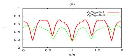
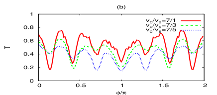
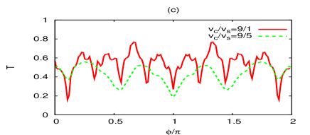
Figure 2: (Color online) Transmission probability for the $g_{4}$-model with $v_{J,c}/v_{s}=v_{c}/v_{s}=q/p$, $v_{J,c}/v_{F}=1$ and $T_{1}/T_{0}=qv_{F}/v_{c}=pv_{F}/v_{s}=5,\-7,\-9$ from top to bottom. The number of prominent dips is always equal to $T_{1}/T_{0}$ with the exception of the case where $v_{c}/v_{s}=9/5$ (see the text). The coupling to the leads is $t^{\prime 2}=0.001$ in these pictures to minimize the dependence of the curves on the energy interval over which the average is taken.

We now proceed and consider situations in which the coupling constants are still chosen such that $v_{c}/v_{s}=q/p$, but $v_{J,c}/v_{F}=v_{c}/v_{F}>1$ (for the $g_{4}$-model with repulsive two-particle interaction). The factor $v_{J,c}$ in front of the magnetic flux in Eq. (36), leads to a decrease of the periodicity of $T(\phi)$ by a factor $v_{F}/v_{J,c}$ and thus to an increase of the number of dips by a factor $v_{J,c}/v_{F}$ with respect to $T_{1}/T_{0}$, the result obtained for $v_{F}=v_{J,c}$. For sufficiently small $q$ and $p$, that is if the “dominant pole” approximation is applicable, we thus expect to find $(v_{J,c}/v_{F})(T_{1}/T_{0})$ dips. This is illustrated in Fig. 3 for $v_{J,c}=v_{c}=3v_{F}/2=3v_{s}$, that is $p=1$, $q=3$.

Figure 3: Transmission probability for the $g_{4}$-model with $v_{c}/v_{s}=3/1$, $v_{J,c}/v_{F}=v_{c}/v_{F}=3/2>1$ and $(v_{J,c}/v_{F})(T_{1}/T_{0})=3$ dips, while $T_{1}/T_{0}=2$.

If the “dominant pole” approximation were applicable for all $p,q$, one would thus have $(v_{J,c}/v_{F})(T_{1}/T_{0})$ dips in $T(\phi)$ in the interval $\phi\in[0,2\pi]$. Given any arbitrary combination of the (relevant) velocities $v_{s}$, $v_{c}$, $v_{J,c}$, a natural strategy for guessing the number of dips would be to look for “small” odd numbers $p$ and $q$ for which $pv_{c}\approx qv_{s}$ and to compute $(v_{J,c}/v_{F})(T_{1}/T_{0})$ from these. The integers $p$ and $q$ would probably be looked for so that $pv_{c}\approx qv_{s}$ holds as accurately as possible for, at the same time, $p$ and $q$ as small as possible. From the dashed line in Fig. 2 (c) it is clear that already the numbers $p=5$ and $q=9$ are not small enough for the “dominant pole” approximation to be reliable. In such cases, one has to resort to smaller odd numbers $p$ and $q$—for which $pv_{c}\approx qv_{s}$ holds less well—to predict the number of dips. As already shown in Fig. 2 (c), for $v_{c}=v_{F}$ and $v_{c}/v_{s}=9/5$, instead of $p=5$ and $q=9$ one has to take $p=3$ and $q=5$ to obtain the correct number of dips. As we shall further show, it is mostly necessary to choose $p$ and $q$ such that for the smaller number $p=1$ even if the approximate identity $pv_{c}\approx qv_{s}$ does then hold only to a very low degree of accuracy. This leads to our central result

$$\left.\frac{v_{J,c}T_{1}}{v_{F}T_{0}}\right|_{p=1}=\frac{v_{J,c}v_{F}}{v_{F}v_{s}}=\frac{v_{J,c}}{v_{s}}$$ (37)

for the number of dips.

Figure 4: Transmission probability for the $g_{4}$-model with the ratio of charge and spin velocities as indicated. In all cases, the number of prominent dips is given by one of the integers closest to $v_{J,c}/v_{s}$ ($=v_{c}/v_{s}$ for the $g_{4}$-model).

Consider, as an example for the validity of Eq. (37), the case where $v_{c}/v_{F}=11v_{s}/(3v_{F})=11/6$ ($p=3$, $q=11$). We then have $T_{1}/T_{0}=pv_{F}/v_{s}=3\cdot 2=6$. Taking into account that $v_{J,c}/v_{F}=v_{c}/v_{F}=11/6$, following the “dominant pole” approximation one would arrive at the conclusion that the number of dips should equal $v_{J,c}T_{1}/(v_{F}T_{0})=11/6\cdot 6=11$. In fact, the numbers $p=3$ and $q=11$ are already too large for this approximation to be valuable. Smaller numbers, for which the equation $pv_{c}=qv_{s}$ is still “approximately” fulfilled, are $p=1$ and $q=3$. This gives $\left.T_{1}/T_{0}\right|_{p=1}=\left.pv_{F}/v_{s}\right|_{p=1}=2$ and thus $\left.(v_{J,c}/v_{F})(T_{1}/T_{0})\right|_{p=1}=11/3$. The number of dips should, of course, be an integer number, and the result $11/3$ lies between $3$ and $4$ so that one can expect one of these two to be the right answer. Indeed, as shown in Fig. 4 (a), the corresponding curve exhibits $3$ dips. This kind of reasoning is applicable whenever the approximate identity $pv_{c}\approx qv_{s}$ does not hold to some sufficiently high degree of accuracy with $p=3,\-5$ and $q=5,\-7$ [as it was the case for the example of the dashed line in Fig. 2 (c)]. We find that Eq. (37) for estimating the number of dips of $T(\phi)$ can be used in almost all cases. Further examples of its validity are shown in Figs. 4 (b), (c) and (d). For Fig. 4 (b) $v_{J,c}/v_{s}=3.8$ and the number of dips is four, while for Fig. 4 (c) $v_{c}/v_{s}=25/2$ so that the numbers $p$ and $q$ for which $pv_{c}=qv_{s}$ are no longer both odd. Equation (37), however, applies nevertheless and, in this case, leads to the result $v_{J,c}/v_{s}=12.5$ again giving a correct estimate of the number of dips.

Jagla and Balseiro argue that, according to the assumptions (“recombination” of spin and charge) underlying their “dominant pole” approximation, the transmission probability would have to be “very small” whenever the couplings are chosen such that $(v_{c}/v_{s})^{\pm 1}=2n$ with integer $n$. In these cases no poles of the form $1/(t-t^{\ast})$ appear in $\mathcal{G}(x=L/2,t)$ and charge and spin excitation cannot “recombine” at finite times at $x=L/2$.Jagla However, the expectation that the transmission probability is small under these conditions is not confirmed by our calculations. Fig. 4 (d) shows the example of a curve for which $v_{c}/v_{s}=4/1$ and in this case (and in all the others we have checked) the transmission probability is not particularly small. This observation provides further evidence that the idea that charge and spin excitations have to “recombine” at $x=L/2$ for an electron to pass through the ring is of very limited usefulness in the present context.

IV.2 Results for the full model

All the results obtained in the model with only $g_{4}$-couplings essentially carry over to the full model (with additional inter-branch interaction $g_{2}$), the main difference being that now $v_{J,c}\neq v_{c}$. The charge current velocity $v_{J,c}$ Eq. (13) becomes smaller than the charge velocity $v_{c}$ due to the presence of nonvanishing $g_{2}$-couplings and it is even reduced to the Fermi velocity if $g_{2,\parallel/\perp}(0)=g_{4,\parallel/\perp}(0)$. An example of such a case is shown in Fig. 5 (a) and the number of dips agrees with the prediction made from Eq. (37) $v_{J,c}/v_{s}=1/0.21\approx 5$.

Figure 5: Transmission probability for the full model and different sets of coupling parameters. The individual couplings are chosen such that the (relevant) velocities are $v_{J,c}/v_{F}=1$, $v_{c}/v_{F}\approx 1.79$, $v_{s}/v_{F}\approx 0.21$ in (a) and $v_{J,c}/v_{F}=v_{s}/v_{F}=1$, $v_{c}/v_{F}\approx 2.01$ in (b).

In case all four couplings $g_{\nu,\parallel/\perp}$ are chosen to be equal, also the spin velocity becomes equal to the Fermi velocity, one then has $v_{s}=v_{J,c}=v_{F}$. The transmission probability for such a case is presented in Fig. 5 (b). It shows a dip structure similar to that of the noninteracting case. This, however, does not come as a surprise in view of the foregoing considerations but is in accordance with Eq. (37) $v_{J,c}/v_{s}=1$.

Figure 6: Transmission probability for couplings such that the (relevant) velocities are $v_{J,c}/v_{F}\approx 1.95$, $v_{s}/v_{F}\approx 0.195$, and $v_{c}/v_{F}\approx 2.32$ leading to $v_{J,c}/v_{s}\approx 1.95/0.195=10$.

Finally, the transmission probability for a more general case is presented in Fig. 6. Here, $T(\phi)$ exhibits $10$ dips and this does indeed represent the ratio of the charge current and the spin velocities following from the chosen coupling constants, namely $v_{J,c}/v_{s}\approx 1.95/0.195=10$.

Our general finding that in most cases $v_{J,c}/v_{s}$ gives an estimate of the number of dips, may be compared to the result of Hallberg et al.Hallberg . They studied the 1d $t$-$J$ model. The Green function of a few lattice site (up to 8 sites) isolated $t$-$J$ ring was computed using exact diagonalization. For $J=0$ this model corresponds to the $U\rightarrow\infty$ - limit of a one-dimensional Hubbard-Hamiltonian for the ring. Whenever the intermediate state contains $N$ electrons, the transmission probability shows $N$ equidistant dips. The authors argue that in the limit $J=0$ the ratio of the spin and charge velocities becomes $v_{c}/v_{s}=N$ and this way try to relate their findings to the ones of Ref. Jagla, . It remains, however, unclear how this would explain the observed dip structure in view of the results presented here which unambiguously suggest that $v_{J,c}$ and not $v_{c}$ is the velocity of importance for the number of dips. In particular, in the $U\rightarrow\infty$ - Hubbard model, one finds $v_{N,c}=2v_{c}$ (see Ref. Schoenhammer05, ) so that $v_{J,c}=1/2v_{c}\neq v_{c}$ [see Eq. (1)].

V Summary

In the present paper we have studied the effect of the different velocities characterizing the low-energy physics of a LL on transport through a one-dimensional, metallic ring of correlated electrons. A magnetic flux piercing the ring was included and the dependence of the transmission probability (linear conductance) on the flux was studied. It was obtained using a relation [Eq. (18)] between the one-particle Green function of the isolated ring and the transmission probability. This becomes exact in the noninteracting limit and serves as an approximation in the presence of two-particle interactions. Results were averaged over a small energy window around the chemical potential just as in Refs. Jagla, and Hallberg, . It proved possible to improve on an approximation suggested in Ref. Jagla, and to exactly calculate the Green functions of the isolated ring for the case of a potential with box-like shape in momentum space. Since only the low-energy properties of the system are relevant, this restriction to a specially shaped potential should not be regarded as severe, in particular because the width of the potential plays practically no role for the results.

Characteristic dips appear in the transmission probability as a function of the magnetic flux whose number depends on the different velocities in play. According to the “dominant pole” approximation of Ref. Jagla, , the number of dips for $\phi\in[0,2\pi]$ is given by $p\,v_{F}/v_{s}=q\,v_{F}/v_{c}$ (or $p\,v_{J,c}/v_{s}=q\,v_{J,c}/v_{c}$ if, as for systems which are not Galilei invariant, $v_{J,c}\neq v_{F}$) if small odd integers $p$ and $q$ can be found such that $pv_{c}=qv_{s}$. For generic repulsive two-particle interactions $v_{s}\leq v_{c}$ and $p$ will be the smaller of the two integers. We have shown that $p$ and $q$ must indeed be very small for this prediction for the number of dips to hold. For more generic choices of the relevant velocities $v_{c}$, $v_{s}$, and $v_{J,c}$, and thus coupling constants, the number of prominent dips in $T(\phi)$ over one interval of periodicity can be estimated to be an integer close to $v_{J,c}/v_{s}$. The wide applicability of this relation was demonstrated.

That the charge current velocity $v_{J,c}$ is a relevant parameter determining the flux dependence of the linear (charge) conductance through the ring should not come as a surprise. The appearance of the velocity of the collective spin excitations $v_{s}$ can be understood from the structure Eqs. (23), (26), (33), and (34) of the one-particle Green function. Generically the sums appearing in these expressions are dominated by the terms in which the integer in front of $v_{c}$ is zero while the integer in front of $v_{s}$ is greater than zero (but small).

A simple picture related to the “dominant pole” approximation suggests that electrons can pass the ring only if spin and charge excitations traveling with different velocities (spin-charge separation) can recombine at the right contact. Our results show that this idea of charge and spin “recombination” is of limited usefulness for the understanding of transport through LL rings.

References

- (1) For a recent review on LL physics see K. Schönhammer in Strong Interactions in Low Dimensions, Eds.: D. Baeriswyl and L. Degiorgi, Kluwer Academic Publishers, Dordrecht (2005).
- (2) E. Jagla, K. Hallberg, and C. Balseiro, Phys. Rev. B 47, 5849 (1993).
- (3) V. Meden and K. Schönhammer, Phys. Rev. B 46, 15753 (1992).
- (4) J. Voit, Phys. Rev. B 47, 6740 (1993).
- (5) C. Kollath, U. Schollwöck, and W. Zwerger, Phys. Rev. Lett. 95, 176401 (2005).
- (6) For a brief review on the experimental situation see Ref. Schoenhammer05, and the article by A. Yacoby in the same book.
- (7) E. Jagla and C. Balseiro, Phys. Rev. Lett. 70, 639 (1993).
- (8) K. Hallberg, A. Aligia, A. Kampf, and B. Normand, Phys. Rev. Lett. 93, 067203 (2004).
- (9) Throughout this work we assume that , which is reasonable for repulsive two-particle interactions (see Ref. Schoenhammer05, ).
- (10) J. Kinaret, M. Jonson, R. Shekter, and S. Eggert, Phys. Rev. B 57, 3777 (1998).
- (11) M. Pletyukhov, V. Gritsev, and N. Pauget, Phys. Rev. B 74, 045301 (2006).
- (12) J. Sólyom, Adv. Phys. 28, 201 (1979).
- (13) For an introduction to bosonization see J. von Delft and H. Schoeller Ann. Phys. (Leipzig) 7, 225 (1998).
- (14) V. Meden, Phys. Rev. B 60, 4571 (1999).
- (15) K. Schönhammer and V. Meden, Phys. Rev. B 47, 16205 (1993).
- (16) D. Loss, Phys. Rev. Lett. 69, 343 (1992).
- (17) P. Schmitteckert, T. Schulze, C. Schuster, P. Schwab, and U. Eckern, Phys. Rev. Lett. 80, 560 (1998).
- (18) V. Meden and U. Schollwöck, Phys. Rev. B 67, 035106 (2003).
- (19) M. Schick, Phys. Rev. 166, 404 (1968).
- (20) T. Enss, V. Meden, S. Andergassen, X. Barnabé-Thériault, W. Metzner, and K. Schönhammer, Phys. Rev. B 71, 155401 (2005).
- (21) S. Friederich, Diploma-thesis, Universität Göttingen, 2007.