Abstract

Two-pion exchange parity-violating nucleon-nucleon interactions from recent effective field theories and earlier fully covariant approaches are investigated. The potentials are compared with the idea to obtain better insight on the role of low-energy constants appearing in the effective field theory approach and the convergence of this one in terms of a perturbative series. The results are illustrated by considering the longitudinal asymmetry of polarized protons scattering off protons, $\vec{p}+p\rightarrow p+p$, and the asymmetry of the photon emission in radiative capture of polarized neutrons by protons, $\vec{n}+p\rightarrow d+\gamma$.

1 Introduction

Effective field theory (EFT) underlies most recent developments in the domain of the nucleon-nucleon ($NN$) strong interaction [1, 2, 3, 4]. The approach is mainly motivated by the fact that a large part of the short-range interaction is essentially unknown. Its detailed description may not be really relevant at low energy and a schematic one, represented by contact interactions with low-energy constants (LEC’s), could be sufficient. Moreover, such an approach could account for important properties in relation to QCD dynamics, i.e. chiral symmetry. Implementing these properties can be done with the chiral perturbation theory [5]. One is thus led to distinguish contributions at different orders. Beyond the one-pion exchange (OPE), which appears at leading order (LO), two-pion exchange (TPE), which is relevant at next-to-next-to-leading order (NNLO), has been considered. Higher order terms are also considered, contributing to a successful description of the strong interaction.

Naturally, the EFT approach has been applied to the weak, parity-violating (PV), $NN$ interaction [6], superposing on earlier phenomenological works in the 70’s [7, 8, 9] with a systematic perturbation scheme in terms of an expansion parameter characterizing the theory. Thus, a one-pion-exchange contribution appears at LO while the two-pion-exchange contribution is part of those at NNLO. It was claimed that effects from the two-pion-exchange contribution could be potentially large. Estimates have been made for various observables [10, 11] and, while they do not contradict the above expectation, they have evidenced a large range of uncertainty [10]. This points out to the role of a contact term present in the operators, which has to be completed in any case by a LEC contribution and cannot be therefore considered as physically relevant by itself. The PV TPE contribution was considered in the 70’s in several works starting from a covariant formalism and based on Feynman diagrams [12] or dispersion relations [13, 14, 15]. Originally, these works were motivated by the expectation that the TPE could play a role in the PV case as important as in the strong interaction one, what was actually disproved by the studies. A similar motivation has recently been addressed within the EFT approach with some attention to the contribution involving the $\Delta$ excitation [16] (see also Refs. [17, 18] with this last respect). Interestingly, the TPE contribution in various processes turned out to be well determined but rather small [13, 15, 19] and, in particular, unessential in comparison with other uncertainties (PV couplings constants, nuclear-structure description, etc). This last feature largely explains its omission in later works. In view of different conclusions, we believe that a comparison of both the recent and earlier works is useful. Some preliminary results were presented in Ref. [20].

The above studies could be relevant because, contrary to the strong interaction, it is not possible to determine at present the LEC’s due to the lack of sufficient and accurate enough experimental data. On the one hand, they could tell us about the role of contact interactions in making the two approaches as close as possible. The contributions of these contact interactions can be ascribed to the LEC or the “finite” range part, depending on the subtraction scheme. On the other hand, they could provide information on the convergence of the perturbative expansion of the potential in the EFT approach, which is limited to NNLO so far. In the field of the strong $NN$ interaction [21] or weak semi-leptonic interactions [22], there are hints for non-negligible corrections.

The plan of this paper is as follows. In the second section, results relative to the TPE contribution from a covariant approach are reminded (isovector part). All components of this interaction and their convergence properties are in particular discussed. The third section is devoted to results in the EFT approach, completed by those obtained from the contribution of time-ordered diagrams as a check. In the fourth section, we examine similarities and differences between results of these approaches and those from an expansion of the covariant one at the lowest non-zero order in the inverse of the nucleon mass, $1/M$. A numerical comparison concerning a few aspects of potentials so obtained is given in the fifth section. Estimates of the effects in two selected processes, proton-proton scattering and radiative neutron-proton capture at thermal energy, are finally given in the sixth section. These two processes allow one to illustrate the two types of PV effects that are expected from the TPE interaction at low energy. The seventh section contains the conclusion. This is completed by appendices concerning the removing of the iterated one-pion exchange and the EFT approach.

2 Two-pion exchange from a covariant formalism

Figure 1: Two-pion exchange in the covariant approach: These diagrams represent the contributions of the crossed box, the non-crossed box and the iterated OPE that has to be subtracted from the previous one. The continuous line represents a baryon and the dashed one a pion. The contributions with nucleon and nucleon resonances in the intermediate state have been considered in the literature. Only the first one is retained here but the role of the other ones will also be mentioned. The PV meson-nucleon vertex is marked with a cross, $\times$. The last diagram on the right represents the iterated one-pion exchange, the back slash indicating that the corresponding nucleon is on-mass shell. Further diagrams with a different order of the parity-violating and parity-conserving meson-nucleon vertices on the same nucleon line, not shown here, are also considered.

We here consider the isovector PV TPE contribution to the $NN$ interaction obtained from a fully covariant formalism. It is induced by an elementary PV pion-nucleon coupling, most often denoted by $h^{1}_{\pi}$. As this coupling also determines the strength of the PV OPE interaction, we give the corresponding expression in terms of both the momentum transfer, $\vec{q}$, and the relative momenta, $\vec{p}$ and $\vec{p}\,^{\prime}$:

$$V_{\pi}(q)=\frac{i\,g_{\pi NN}\;h^{1}_{\pi}}{2\sqrt{2}\,M}\;(\tau_{1}\!\times\!\tau_{2})^{z}\;\frac{(\vec{\sigma}_{1}\!+\!\vec{\sigma}_{2})\!\cdot\!(\vec{p}\,^{\prime}\!-\!\vec{p}\,)}{m^{2}_{\pi}+q^{2}}=-\frac{i\,g_{\pi NN}\;h^{1}_{\pi}}{2\sqrt{2}\,M}\;(\tau_{1}\!\times\!\tau_{2})^{z}\;\frac{(\vec{\sigma}_{1}\!+\!\vec{\sigma}_{2})\!\cdot\!\vec{q}}{m^{2}_{\pi}+q^{2}}\,.$$ (1)

Due to possible ambiguity, we further specify the notations for momenta:

$$\vec{p}=\frac{1}{2}\,(\vec{p}_{1}-\vec{p}_{2}),\;\;\vec{p}\,^{\prime}=\frac{1}{2}\,(\vec{p}\,^{\prime}_{1}-\vec{p}\,^{\prime}_{2})\,,$$

$$\vec{q}=(\vec{p}_{1}-\vec{p}\,^{\prime}_{1})=-(\vec{p}_{2}-\vec{p}\,^{\prime}_{2})=(\vec{p}-\vec{p}\,^{\prime})\,,$$ (2)

where the primed and non-primed momenta refer to those of particles appearing respectively in the bra and ket states. In configuration space, the interaction thus recovers its standard form:

$$V_{\pi}(r) = \frac{i\,g_{\pi NN}\;h^{1}_{\pi}}{2\sqrt{2}\,M}\;(\tau_{1}\times\tau_{2})^{z}\;\;(\vec{\sigma}_{1}\!+\!\vec{\sigma}_{2})\!\cdot\Big{[}\vec{p},\;\frac{e^{-m_{\pi}r}}{4\pi\,r}\Big{]}$$ (3)

$$= -\frac{\,g_{\pi NN}\;h^{1}_{\pi}}{2\sqrt{2}\,M}\;(\tau_{1}\times\tau_{2})^{z}\;\;(\vec{\sigma}_{1}\!+\!\vec{\sigma}_{2})\!\cdot\!(\vec{r_{1}}\!-\!\vec{r_{2}})\;\frac{e^{-m_{\pi}r}(1\!+\!m_{\pi}r)}{4\pi\,r^{3}}\,,$$

with $r=|\vec{r_{1}}-\vec{r_{2}}|$. First studies of the isovector PV TPE contribution were made in the early 70’s [12, 13, 14, 15]. For a part, they were motivated by the underestimation of some observed PV effects using the standard PV $NN$ interaction available at that time. Similarly to the strong-interaction case, where the TPE contribution is quantitatively more important than the OPE one, it was believed that the TPE contribution could also play an essential role in the PV case.

Various studies roughly agree with each other, after correcting mistakes in some cases [12, 14]. Differences involve in particular the formalism (calculations using Feynman diagrams or dispersion relations), non-relativistic approximations in external nucleon lines, or the removing of the OPE-iterated contribution in the box diagram. The choice of the Green’s function in the last ingredient was rather unimportant due to the introduction of cutoffs in applications. It could however be important in unrestricted calculations. The point is of relevance with respect to a comment made in Ref. [6] about the absence of convergence in earlier calculations. It will be discussed in more detail below when expressions for the TPE contribution are given.

The crossed and non-crossed box diagrams that enter the isovector TPE contribution of interest here are represented in Fig. 1, where the intermediate hadron on the upper line can be a nucleon as well as a resonance ($\Delta(1231),\;N^{*}(1440),\;N^{*}(1518)$). For our purpose and also for simplicity, we only retain the nucleon. Altogether, the corresponding contribution to the isovector interaction involves six different terms. Following for a part the notations of Ref. [15], it can be written quite generally in momentum space as:

$$V(\vec{p}\,^{\prime},\vec{p})=V_{44}+V_{34}+V_{56}+V_{75}+V_{66}+V_{85}$$

$$\hskip 8.53581pt=i\,(\tau_{1}+\tau_{2})^{z}\;\;(\vec{\sigma}_{1}\times\vec{\sigma}_{2})\!\cdot\!(\vec{p}\,^{\prime}-\vec{p})\;v_{44}(q,\cdots)$$

$$\hskip 17.07164pt+\,(\tau_{1}+\tau_{2})^{z}\;\;(\vec{\sigma}_{1}-\vec{\sigma}_{2})\!\cdot\!(\vec{p}\,^{\prime}+\vec{p})\;v_{34}(q,\cdots)$$

$$\hskip 17.07164pt+i\,(\tau_{1}\times\tau_{2})^{z}\;\;(\vec{\sigma}_{1}+\vec{\sigma}_{2})\!\cdot\!(\vec{p}\,^{\prime}-\vec{p})\;v_{56}(q,\cdots)$$

$$\hskip 17.07164pt+\,(\tau_{1}-\tau_{2})^{z}\;\;(\vec{\sigma}_{1}+\vec{\sigma}_{2})\!\cdot\!(\vec{p}\,^{\prime}+\vec{p})\;v_{75}(q,\cdots)$$

$$\hskip 17.07164pt+\,(\tau_{1}\!\times\!\tau_{2})^{z}\;\;\Big{(}\vec{\sigma}_{1}\!\cdot\!\vec{q}\;\vec{\sigma}_{2}\!\cdot\!(\vec{p}\,^{\prime}\!+\!\vec{p})\!\times\!\vec{q}+(\vec{\sigma}_{1}\leftrightarrow\vec{\sigma}_{2})\Big{)}\;v_{66}(q,\cdots)$$

$$\hskip 17.07164pt-i\,(\tau_{1}\!-\!\tau_{2})^{z}\;\;\Big{(}\vec{\sigma}_{1}\!\cdot\!(\vec{p}\,^{\prime}\!+\!\vec{p})\;\vec{\sigma}_{2}\!\cdot\!(\vec{p}\,^{\prime}\!+\!\vec{p})\!\times\!\vec{q}+(\vec{\sigma}_{1}\leftrightarrow\vec{\sigma}_{2})\Big{)}\;v_{85}(q,\cdots)\,.$$ (4)

Functions $v_{ij}(q,\cdots)$ assume a dispersion-relation form:

$$v^{\rm COV}_{ij}(q,\cdots)=\frac{1}{\pi}\int_{4m^{2}_{\pi}}^{\infty}dt^{\prime}\;\frac{g_{ij}(t^{\prime},\cdots)}{\sqrt{t^{\prime}}\;(t^{\prime}+q^{2})}\,,$$ (5)

and dots represent possible extra dependence on $\vec{p}\,^{\prime}$ and $\vec{p}$ (kinetic energy in particular).

The configuration-space PV TPE potential is obtained from the standard relation:

$$v(r)=\int\frac{d\vec{q}}{(2\pi)^{3}}\,e^{-i\vec{q}\cdot\vec{r}}\,v(q)\,.$$ (6)

Its expression thus reads:

$$V(r,\vec{p}\,^{\prime},\vec{p})=i\,(\tau_{1}+\tau_{2})^{z}\;\;(\vec{\sigma}_{1}\times\vec{\sigma}_{2})\!\cdot\![\vec{p},\;v_{44}(r,\cdots)]$$

$$\hskip 8.53581pt+\,(\tau_{1}+\tau_{2})^{z}\;\;(\vec{\sigma}_{1}-\vec{\sigma}_{2})\!\cdot\!\{\vec{p},\;v_{34}(r,\cdots)\}$$

$$\hskip 8.53581pt+i\,(\tau_{1}\times\tau_{2})^{z}\;\;(\vec{\sigma}_{1}+\vec{\sigma}_{2})\!\cdot\![\vec{p},\;v_{56}(r,\cdots)]$$

$$\hskip 8.53581pt+\,(\tau_{1}-\tau_{2})^{z}\;\;(\vec{\sigma}_{1}+\vec{\sigma}_{2})\!\cdot\!\{\vec{p},\;v_{75}(r,\cdots)\}$$

$$\hskip 8.53581pt+2i\,(\tau_{1}\!\times\!\tau_{2})^{z}\;\;\Big{(}\vec{\sigma}_{1}\!\cdot\![\vec{p},\,\vec{\sigma}_{2}\!\cdot\!\vec{l}\;\frac{1}{r}\frac{d}{dr}v_{66}(r,\cdots)]+(\vec{\sigma}_{1}\leftrightarrow\vec{\sigma}_{2})\Big{)}\;$$

$$\hskip 8.53581pt-2\,(\tau_{1}\!-\!\tau_{2})^{z}\;\;\Big{(}\vec{\sigma}_{1}\!\cdot\!\{\vec{p},\,\vec{\sigma}_{2}\!\cdot\!\vec{l}\;\frac{1}{r}\frac{d}{dr}v_{85}(r,\cdots)\}+(\vec{\sigma}_{1}\leftrightarrow\vec{\sigma}_{2})\Big{)}\;\,,$$ (7)

where:

$$v^{\rm COV}_{ij}(r,\cdots)=\frac{1}{4\pi^{2}}\int_{4m^{2}_{\pi}}^{\infty}dt^{\prime}\;g_{ij}(t^{\prime},\cdots)\;\frac{e^{-r\sqrt{t^{\prime}}}}{r\;\sqrt{t^{\prime}}}\,,$$ (8)

while $\vec{p}\,^{\prime}$ and $\vec{p}$, which dots account for, have now an operator character and should be placed respectively on the left and the right, in accordance with our conventions.

The terms $V_{44}$, $V_{34}$, $V_{56}$ and $V_{75}$ appear at the first order in a $p/M$ expansion of the Lorentz invariants appearing in the expression of the interaction. The two other ones, $V_{66}$ and $V_{85}$, appear at the third order in $p/M$. They can therefore be considered as relativistic corrections. Moreover, they only contribute when going beyond the transitions between lowest partial wave states, i.e. $S$ to $P$, which generally dominate at low energy (where most PV data are available). For these two reasons, the corresponding terms were discarded in the past, which we also do here. We however stress that these higher-order terms are necessary to get a full mapping of the $NN$ interaction, especially to discriminate transitions involving higher partial waves such as ${}^{3}P_{1}\!-\!\!\,^{3}D_{1}$ and ${}^{3}P_{2}\!-\!\!\,^{3}D_{2}$, ${}^{3}D_{2}\!-\!\!\,^{3}F_{2}$ and ${}^{3}D_{3}\!-\!\!\,^{3}F_{3}$, etc. It is also noticed that the above non-relativistic expansion only involves the nucleon external lines, as done in other approaches. None is made for internal nucleon lines where big effects could arise. As our results presented in this paper only retain part of the full relativistic structure, they will be denoted “covariant” to avoid overstating this property.

We now consider the expressions of the $V_{44}$, $V_{34}$, $V_{56}$ and $V_{75}$ terms. It is first noticed that $V_{44}$ and $V_{34}$ only receive contribution from the crossed diagram while $V_{56}$ and $V_{75}$ also get some from the non-crossed one. In this case, one has therefore to worry about the removing of the iterated OPE and, especially, about the choice of the Green’s function which enters the calculation. In Ref. [13], the Green’s function, $(2E_{0}-2E)^{-1}$, was used, taking into account that the Schrödinger equation is linear in the energy of the system, $E_{0}$, and assuming moreover that the kinetic energy of particles retains its relativistic form ($E=\sqrt{M^{2}+p^{2}}$ in the c.m.). In later works [14, 15], a Green’s function more in agreement with a non-relativistic Schrödinger equation, $E/(p_{0}^{2}-p^{2})$, was instead used. The difference, a factor $2E/(E_{0}+E)$, had minor numerical effects in the past calculations where cutoffs were introduced in the dispersion integrals, Eq. (5). The difference however matters in unrestricted calculations. Dispersion-relation integrals diverge in the first case while they converge in the second one. With this last respect, it is noticed that the corresponding Green’s function can be written in the following form, $E/(E_{0}^{2}-E^{2})$, which rather evokes an equation with a quadratic-mass operator. Such an equation is known to provide solutions with a behavior in the relativistic domain better than the linear one [23]. This is the choice made here. Taking into account that the kinetic-energy dependence is small, and that we are interested in low-energy processes, the momentum in functions $g(q,\cdots)$ can be set to 0. In a similar way as Ref. [13] with details given in Appendix A.1, the closed expressions for these functions are then obtained. Omitting dots that are no longer justified, they read:

$$g_{44}(t^{\prime}) = \tilde{K}\frac{1}{2M}\Bigg{(}\frac{4q_{\pi}}{\chi^{2}}+\frac{H}{M^{2}}-G\Big{(}\frac{1}{M^{2}}+\frac{1}{\chi^{2}}\Big{)}\Bigg{)}\,,$$

$$g_{34}(t^{\prime}) = \tilde{K}\frac{1}{2M^{3}}\Bigg{(}G-\frac{H\;x^{2}}{x^{2}+4M^{2}q_{\pi}^{2}}\Bigg{)}\,,$$

$$g_{56}(t^{\prime}) = -\tilde{K}\frac{1}{2M}\;\frac{H\;x}{x^{2}+4M^{2}q_{\pi}^{2}}-\tilde{K}\frac{x}{M^{2}\;m^{2}_{\pi}}\;{\rm arctg}\Big{(}\frac{m^{2}_{\pi}}{2Mq_{\pi}}\Big{)}$$

$$\!\!+\tilde{K}\int_{k_{-}^{2}}^{{k_{+}^{2}}}\frac{dk^{2}}{\sqrt{k^{2}t^{\prime}\!-\!(m^{2}_{\pi}\!+\!k^{2})^{2}}}\;\frac{1}{2E\,(E\!+\!M)}\Bigg{(}\frac{x}{M^{2}}\!+\!\frac{k^{2}}{M\,(E\!+\!M)}\Bigg{)}\,,$$

$$g_{75}(t^{\prime}) = \tilde{K}\frac{4x^{2}}{M^{2}\,m^{2}_{\pi}\,t^{\prime}}\;{\rm arctg}\Big{(}\frac{m^{2}_{\pi}}{2Mq_{\pi}}\Big{)}+\tilde{K}\frac{2G}{Mt^{\prime}}$$ (9)

$$\!\!-\tilde{K}\int_{k_{-}^{2}}^{{k_{+}^{2}}}\frac{dk^{2}}{\sqrt{k^{2}t^{\prime}\!-\!(m^{2}_{\pi}\!+\!k^{2})^{2}}}$$

$$\hskip 8.53581pt\times\frac{2}{E(E\!+\!M)}\Bigg{(}\frac{x^{2}}{M^{2}t^{\prime}}\!+\!\frac{2E\,x}{Mt^{\prime}}\!-\!\frac{k^{2}}{M(E\!+\!M)}\!-\!\frac{k^{4}}{M(E\!+\!M)t^{\prime}}\Bigg{)}\,,$$

where:

$$\tilde{K} = \frac{g^{3}_{\pi\,NN}\;h^{1}_{\pi}}{32\pi\sqrt{2}}\,,$$

$$q_{\pi} = \sqrt{\frac{t^{\prime}}{4}-m^{2}_{\pi}},\hskip 28.45274pt\chi^{2}=M^{2}-\frac{t^{\prime}}{4},\hskip 28.45274ptx=\frac{t^{\prime}}{2}-m^{2}_{\pi}\,,$$

$$H = 2\sqrt{\frac{x^{2}+4M^{2}q_{\pi}^{2}}{t^{\prime}}}\;\;{\rm ln}\Bigg{(}\frac{\sqrt{x^{2}+4M^{2}q_{\pi}^{2}}+q_{\pi}\sqrt{t^{\prime}}}{\sqrt{x^{2}+4M^{2}q_{\pi}^{2}}-q_{\pi}\sqrt{t^{\prime}}}\Bigg{)}\,,$$

$$G = \frac{2x}{\chi}\;{\rm arctg}\Big{(}\frac{2q_{\pi}\chi}{x}\Big{)}\;\;\;[\chi^{2}\geq 0],\;\;\;=\frac{x}{\sqrt{\!-\!\chi^{2}}}\;{\rm ln}\Bigg{(}\frac{x+2q_{\pi}\sqrt{\!-\!\chi^{2}}}{x-2q_{\pi}\sqrt{\!-\!\chi^{2}}}\Bigg{)}\;\;\;[\chi^{2}\leq 0]\,,$$

$$k_{\pm}^{2} = x\pm q_{\pi}\sqrt{t^{\prime}},\hskip 28.45274ptE=\sqrt{M^{2}+k^{2}}\,.$$ (10)

Looking at the asymptotic behavior of the functions $g_{ij}(t^{\prime})$ for large $t^{\prime}$, it is noticed that the dominant contributions of individual terms, $\propto t^{\prime 1/2}$, as well as the constant ones, cancel (see Appendix A.2 for some detail). One is thus left with the following contributions:

$$g_{44}(t^{\prime})_{t^{\prime}\rightarrow\infty} = \tilde{K}\frac{2}{M\sqrt{t^{\prime}}}\Bigg{(}{\rm ln}\Big{(}\frac{t^{\prime}}{M^{2}}\Big{)}-1\Bigg{)}\,,$$

$$g_{34}(t^{\prime})_{t^{\prime}\rightarrow\infty} = \tilde{K}\frac{2}{M\sqrt{t^{\prime}}}\Bigg{(}{\rm ln}\Big{(}\frac{t^{\prime}}{M^{2}}\Big{)}-1\Bigg{)}\,,$$

$$g_{56}(t^{\prime})_{t^{\prime}\rightarrow\infty} = -\tilde{K}\frac{1}{M\sqrt{t^{\prime}}}\Bigg{(}\frac{5}{8}\,{\rm ln}\Big{(}\frac{t^{\prime}}{M^{2}}\Big{)}+\frac{15}{8}-\frac{3}{2}\,{\rm ln}(2)\Bigg{)}\,,$$

$$g_{75}(t^{\prime})_{t^{\prime}\rightarrow\infty} = \tilde{K}\frac{1}{M\sqrt{t^{\prime}}}\Bigg{(}\frac{9}{4}\,{\rm ln}\Big{(}\frac{t^{\prime}}{M^{2}}\Big{)}-\frac{1}{4}+\,{\rm ln}(2)\Bigg{)}\,.$$ (11)

In all cases, the functions $g_{ij}(t^{\prime})$ behave asymptotically as $t^{\prime-1/2}$, up to log terms, ensuring the convergence of the integrals given in Eq. (5). This result is important as it allows one to consider the dispersion approach as a benchmark, thus providing information about contributions that are ascribed to LEC’s as well as possible higher-order corrections in other approaches.

3 Two-pion exchange from the EFT approach

3.1 EFT approach

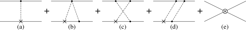
Figure 2: One and two-pion exchange in the EFT approach: The contributions from the OPE (a), from the triangle TPE (b), from the crossed TPE (c), from the non-crossed TPE (d) and from the contact term (e). See the caption of Fig. 1 for further comments.

The PV TPE at NNLO has been calculated in the EFT approach by Zhu et al. [6]. It contains two components which, in their notations, involve functions $\tilde{C}^{2\pi}_{2}(q)$ and $C^{2\pi}_{6}(q)$ and correspond here to the components $V_{44}$ and $V_{56}$ of the more complete interaction given by Eq. (4). The contributions being accounted for correspond to the diagrams shown in Fig. 2. Their expressions for the finite-range part and the associated contact term have been obtained in the maximal-subtraction (MX) scheme. Factorizing out the spin-isospin dependence and taking into account corrections made since then [10], they read: 

$$v_{44}^{\rm EFT}(q) \!=\! -4\sqrt{2}\;\pi\frac{h^{1}_{\pi}}{\Lambda^{3}_{\chi}}\Big{(}g_{A}^{3}\,L(q)\Big{)}\,,$$

$$v_{56}^{\rm EFT}(q) \!=\! -\sqrt{2}\;\pi\frac{h^{1}_{\pi}}{\Lambda^{3}_{\chi}}\Bigg{(}g_{A}\;L(q)-g_{A}^{3}\;\Big{(}3L(q)\!-\!H(q)\Big{)}\Bigg{)}\,,$$ (12)

where the scale $\Lambda_{\chi}$ is roughly given by $\Lambda_{\chi}=4\pi f_{\pi}\simeq 4\pi\,g_{A}\,M/g_{\pi NN}\simeq 1$ GeV. The $L(q)$ and $H(q)$ functions are defined as:

$$L(q)=\frac{\sqrt{q^{2}\!+\!4m_{\pi}^{2}}}{q}\,\ln\!\left(\frac{\sqrt{q^{2}\!+\!4m_{\pi}^{2}}+q}{2m_{\pi}}\right)=\frac{\sqrt{q^{2}\!+\!4m_{\pi}^{2}}}{2\,q}\,\ln\!\left(\frac{\sqrt{q^{2}\!+\!4m_{\pi}^{2}}+q}{\sqrt{q^{2}\!+\!4m_{\pi}^{2}}-q}\right)\,,$$

$$H(q)=\frac{4m_{\pi}^{2}}{q^{2}\!+\!4m_{\pi}^{2}}\;L(q)\,.$$ (13)

The detail of the contributions corresponding to the diagrams (b), (c) and (d) in Fig. 2 can be found in Appendix B. The above terms entering the interaction should be completed by contact terms:

$$v^{CT}_{44}=C_{44}\,,$$

$$v^{CT}_{56}=C_{56}\,.$$ (14)

The contributions from two-pion exchange to these contact terms are also given in Appendix B, where it is seen that they require some renormalization. The sum of the EFT two-pion-exchange and contact contributions should be well determined, but how it is split between the two terms is not. In the minimal-subtraction ($\overline{\mbox{\rm MS}}$) scheme, the part of the contact term which is proportional to $1\!+\!{\rm ln}(\mu/m_{\pi})$ (see Appendix B) is shifted to the EFT two-pion-exchange part. In such a case, the term “1” cancels the function $L(q)$ at $q=0$ and the log term, for $\mu\geq m_{\pi}$, changes the overall sign of the potential in the low-$q$ range.

3.2 Relation to the time-ordered-diagram approach

Figure 3: Two-pion exchange in the time-ordered diagram approach: The contributions from the crossed diagrams (the first line), from the Z-type contributions (the second line, identified as triangle diagrams in a different approach), from the non-crossed diagrams (the diagrams on the third line). The last two diagrams differ in that the first of them involves a meson propagator with off-energy shell contributions, which are omitted in the other one (what is reminded by a back slash on the meson lines). This last contribution, which arises from the iterated OPE, has to be subtracted from the previous one. The discrepancy involves a factor, $E_{0}-k^{2}/M$, which cancels a similar factor entering the denominator of the Green function ($\vec{k}$ can be identified as the loop momentum). See the caption of Fig. 1 for further comments.

When integrating the EFT expressions of the TPE interaction over the time component of the integration variable entering some loop, it is expected that one should recover expressions obtained from considering time-ordered (TO) diagrams in the non-relativistic limit ($\vec{v}\rightarrow 0$ where $\vec{v}$ is the nucleon velocity $\vec{v}\simeq\vec{p}/M$). As this check was quite useful in determining the correct expressions given in the previous subsection, we give below the raw expressions obtained from the contribution of these time-ordered diagrams, which are shown in Fig. 3. Starting from the elementary $\pi NN$ interaction, $g_{\pi NN}\,\vec{\sigma}\cdot\vec{k}/(2M\,\sqrt{\omega_{k}})$ (with $\omega_{k}=\sqrt{m_{\pi}^{2}+k^{2}}$), one gets:

$$v^{\rm TO}_{44}(q) \!=\! \frac{g_{\pi NN}^{3}\;h^{1}_{\pi}}{4\sqrt{2}\,M^{3}}\;\;$$

$$\times\int\frac{d\vec{k}}{(2\pi)^{3}}\frac{k^{2}\!-\!(\vec{k}\cdot\hat{q})^{2}}{\omega_{i}\;\omega_{j}}\;\Bigg{(}\frac{1}{\omega_{i}^{2}\,(\omega_{i}\!+\!\omega_{j})}+\frac{1}{(\omega_{i}\!+\!\omega_{j})\,\omega^{2}_{j}}+\frac{1}{\omega_{i}\,(\omega_{i}\!+\!\omega_{j})\,\omega_{j}}\Bigg{)}\,,$$

$$v^{\rm TO}_{56}(q) \!=\! \frac{g_{\pi NN}^{3}\;h^{1}_{\pi}}{4\sqrt{2}\,M^{3}}\;\;\Bigg{(}\frac{1}{2}\int\frac{d\vec{k}}{(2\pi)^{3}}\frac{1}{\omega_{i}\,\omega_{j}\,(\omega_{i}\!+\!\omega_{j})}$$ (15)

$$-\frac{1}{2}\int\frac{d\vec{k}}{(2\pi)^{3}}\;\frac{k^{2}\!-\!\frac{q^{2}}{4}}{\omega_{i}\;\omega_{j}}\;\Bigg{(}\frac{1}{\omega_{i}^{2}\,(\omega_{i}\!+\!\omega_{j})}+\frac{1}{(\omega_{i}\!+\!\omega_{j})\,\omega^{2}_{j}}+\frac{1}{\omega_{i}\,(\omega_{i}\!+\!\omega_{j})\,\omega_{j}}\Bigg{)}\Bigg{)}\,,$$

where $\omega_{i}=\sqrt{m^{2}_{\pi}+(\vec{k}+\vec{q}/2)^{2}}$, $\omega_{j}=\sqrt{m^{2}_{\pi}+(\vec{k}-\vec{q}/2)^{2}}$. The three integrals involve the contributions successively from the crossed diagrams (the first line of Fig. 3), Z-type ones (the second line of Fig. 3) and both crossed and non-crossed diagrams (the first and third lines of Fig. 3). The Z-type diagrams are calculated assuming a pseudo-scalar coupling, consistently with the dispersion-relation approach used independently, and retaining the lowest non-zero term in a $1/M$ expansion. As is known, the contribution alone violates chiral symmetry (see, for instance, Ref. [24]). The expected symmetry is restored by further contributions, which can be calculated in the same formalism (see some detail in Sec. 4.2). Contributions of all diagrams in Fig. 3 diverge but they contain a well-defined part that can be analytically calculated. Interestingly, the expressions so obtained can be cast into the form of dispersion integrals. This property stems from considering a complete set of topologically-equivalent time-ordered diagrams. This writing is interesting as it greatly facilitates the comparison with the expressions obtained from a covariant approach, which evidences the same form. It is thus found that the different integrals in Eqs. (15) read:

$$\int d\vec{k}\;\frac{k^{2}\!-\!(\vec{k}\cdot\hat{q})^{2}}{\omega_{i}\;\omega_{j}}\;\Bigg{(}\frac{1}{\omega_{i}^{2}\,(\omega_{i}\!+\!\omega_{j})}+\frac{1}{(\omega_{i}\!+\!\omega_{j})\,\omega^{2}_{j}}+\frac{1}{\omega_{i}\,(\omega_{i}\!+\!\omega_{j})\,\omega_{j}}\Bigg{)}$$

$$\hskip 28.45274pt=4\pi\Big{(}1-L(q)\Big{)}+\int d\vec{k}\,\frac{k^{2}}{\omega_{k}^{5}}=\pi\int_{4m_{\pi}^{2}}^{\infty}dt^{\prime}\;\frac{2\sqrt{t^{\prime}-4\,m_{\pi}^{2}}}{\sqrt{t^{\prime}}\;(t^{\prime}+q^{2})}\,,$$

$$\int d\vec{k}\;\frac{1}{\omega_{i}\,\omega_{j}\,(\omega_{i}\!+\!\omega_{j})}$$

$$\hskip 28.45274pt=2\pi\Big{(}1-L(q)\Big{)}+\frac{1}{2}\int d\vec{k}\,\frac{1}{\omega_{k}^{3}}=\pi\int_{4m_{\pi}^{2}}^{\infty}dt^{\prime}\;\frac{\sqrt{t^{\prime}-4\,m_{\pi}^{2}}}{\sqrt{t^{\prime}}\;(t^{\prime}+q^{2})}\,,$$

$$\int d\vec{k}\;\frac{k^{2}\!-\!\frac{q^{2}}{4}}{\omega_{i}\;\omega_{j}}\;\Bigg{(}\frac{1}{\omega_{i}^{2}\,(\omega_{i}\!+\!\omega_{j})}+\frac{1}{(\omega_{i}\!+\!\omega_{j})\,\omega^{2}_{j}}+\frac{1}{\omega_{i}\,(\omega_{i}\!+\!\omega_{j})\,\omega_{j}}\Bigg{)}\Bigg{)}$$

$$\hskip 28.45274pt=2\pi\Bigg{(}3\Big{(}1-L(q)\Big{)}+H(q)\Bigg{)}+\frac{3}{2}\int d\vec{k}\,\frac{k^{2}}{\omega_{k}^{5}}$$

$$\hskip 28.45274pt=\pi\int_{4m_{\pi}^{2}}^{\infty}dt^{\prime}\;\;\frac{3(t^{\prime}\!-\!4m_{\pi}^{2})+4m_{\pi}^{2}}{\sqrt{t^{\prime}}\;\sqrt{t^{\prime}\!-\!4m_{\pi}^{2}}\;(t^{\prime}\!+\!q^{2})}\,.$$ (16)

Due to the divergent character of these integrals, the above equalities hold up to some constant. This does not however affect the $q^{2}$-dependent part. One can thus remove an infinite contribution so that the interaction takes a definite value at some $q^{2}$. A particular interesting choice is to subtract a part so that the remaining one, which contains the most physically relevant part, cancels at $q^{2}\!=\!0$. By looking at this quantity, one can usefully compare different approaches. To some extent the slope with respect to $q^{2}$ at $q^{2}\!=\!0$ provides information on the sign and the strength of the interaction at finite distances. The $L(q)$ function in the above equalities thus points to a configuration-space interaction with an opposite sign at finite distances. The divergent part is not without interest however. It tells us in which direction the (short-range) subtracted interaction is likely to contribute. By integrating out the contribution $t^{\prime}\geq\tilde{\Lambda}^{2}$ at the r.h.s. of Eqs. (16) in the small $q$ limit, one successively gets the approximate factors $4\pi\,{\rm ln}(\tilde{\Lambda}/2m_{\pi})$, $2\pi\,{\rm ln}(\tilde{\Lambda}/2m_{\pi})$, and $6\pi\,{\rm ln}(\tilde{\Lambda}/2m_{\pi})$. This suggests two observations. On the one hand, for large enough $\tilde{\Lambda}$, the r.h.s. has a sign opposite to that one given by the $L(q)$ term at the l.h.s., confirming the observation in configuration space. On the other hand, the above factor allows one to make some relation with the EFT interaction calculated in the minimal-subtraction scheme, which involves similar log terms (with $\tilde{\Lambda}$ replaced by $\mu$).

Comparing the above expressions, Eqs. (16), with the previous EFT ones, Eqs. (12), it is found that the $q^{2}$ dependences are very similar. Assuming the choice $\Lambda_{\chi}=4\pi\,g_{A}\,M/g_{\pi NN}$, an identity is actually found for the potential, $v_{44}(q)$, as well as the second term for the other potential, $v_{56}(q)$. For the first term in $v_{56}(q)$, which can be associated with a triangle-type diagram, the time-ordered diagram approach used here gives a factor $g_{A}^{3}$ instead of $g_{A}$ as directly obtained from the Weinberg-Tomozawa term. This discrepancy points to the fact that the approach misses some contribution. As already mentioned, this will be discussed in more details in Sec. 4.2 when making a comparison with the expressions obtained from the covariant formalism.

4 Relation of the EFT approach to the covariant one

We here discuss similarities and differences between the expressions obtained from the full covariant approach and the EFT one presented in sections 2 and 3 respectively.

4.1 Similarities (large-$M$ limit)

To make a comparison of the EFT and time-ordered-diagram approaches with the covariant one, the first step is to derive expressions in the large-$M$ limit for the last case. Taking this limit in the simplest-minded way for the $H$ and $G$ functions given in Eq. (10), one gets:

$$H_{M\rightarrow\infty} = 4\,q_{\pi}=2\sqrt{t^{\prime}-4m^{2}_{\pi}}\,,$$

$$G_{M\rightarrow\infty} = \frac{(t^{\prime}-2m^{2}_{\pi})}{M}\Bigg{(}\frac{\pi}{2}-\frac{x}{2q_{\pi}M}\Bigg{)}\simeq\pi\frac{x}{M}\,.$$ (17)

Inserting the above limits in Eqs. (9), one finds:

$$g_{44}(t^{\prime})_{M\rightarrow\infty} \!=\! \tilde{K}\;\frac{4q_{\pi}}{M^{3}}=\tilde{K}\;\frac{2\sqrt{t^{\prime}\!-\!4m^{2}_{\pi}}}{M^{3}}\,,$$

$$g_{34}(t^{\prime})_{M\rightarrow\infty} \!=\! \tilde{K}\;\frac{\pi}{M^{4}}\,\frac{x}{2}=\tilde{K}\;\frac{\pi}{M^{4}}\frac{t^{\prime}\!-\!2m^{2}_{\pi}}{4}\,,$$

$$g_{56}(t^{\prime})_{M\rightarrow\infty} \!=\! -\tilde{K}\;\frac{x}{q_{\pi}\,M^{3}}=-\tilde{K}\;\frac{(t^{\prime}\!-\!2m^{2}_{\pi})}{M^{3}\,\sqrt{t^{\prime}\!-\!4m^{2}_{\pi}}}\,,$$

$$g_{75}(t^{\prime})_{M\rightarrow\infty} \!=\! \tilde{K}\;\frac{\pi}{M^{4}}\;(\frac{t^{\prime}-4m^{2}_{\pi}}{16}+\frac{3}{2}\,\frac{t^{\prime}-2m^{2}_{\pi}}{4})\,.$$ (18)

In obtaining the above expressions, one has taken into account that the integral in Eq. (9) for $g_{56}(t^{\prime})$ has a higher $1/M$ order ($1/M^{4}$). The case of $g_{75}(t^{\prime})$ is more complicated as individual contributions of $1/M^{2}$ and $1/M^{3}$ order cancel. In any case, we notice that the large-$M$ limit does not commute with the large-$t^{\prime}$ limit (compare with the results given in Eq. (11)). Differences from the “covariant” results are therefore expected when considering short distances, where the last limit is relevant. The insertion of the above limits in the dispersion-relation integrals, Eqs. (5), allows one to recover the expressions of the time-ordered-diagram approach at the lowest order, $1/M^{3}$, for interactions $V_{44}$ and $V_{56}$:

$$v_{44}(q)_{M\rightarrow\infty}=\frac{g_{\pi NN}^{3}\;h^{1}_{\pi}}{16\sqrt{2}\;\pi^{2}\,M^{3}}\;\;\int_{4m^{2}_{\pi}}^{\infty}dt^{\prime}\;\frac{\sqrt{t^{\prime}-4\,m^{2}_{\pi}}}{\sqrt{t^{\prime}}\,(t^{\prime}+q^{2})}\,,$$

$$v_{56}(q)_{M\rightarrow\infty}=-\;\frac{g_{\pi NN}^{3}\;h^{1}_{\pi}}{32\sqrt{2}\;\pi^{2}\,M^{3}}\;\int_{4m^{2}_{\pi}}^{\infty}dt^{\prime}\;\frac{(t^{\prime}\!-\!2m^{2}_{\pi})}{\sqrt{t^{\prime}}\;\sqrt{t^{\prime}\!-\!4m^{2}_{\pi}}\;(t^{\prime}\!+\!q^{2})}\,.$$ (19)

For the interaction $V_{56}$, it is noticed that the two terms involving integrands proportional to $-(t^{\prime}\!-\!4m^{2}_{\pi})$ and $3(t^{\prime}\!-\!4m^{2}_{\pi})+4m^{2}_{\pi}$ in Eq. (15) (together with Eq. (16)) combine to give the factor proportional to $(t^{\prime}\!-\!2m^{2}_{\pi})$ appearing in the large-$M$-limit expression of $g_{56}(t^{\prime})$, Eq. (18).

Expressions for both $V_{44}$ and $V_{56}$ can be cast into a form that facilitates the comparison with Zhu et al.’s work [6]. In this order, a factor $g_{\pi NN}^{3}/(4\,\pi g_{A}M)^{3}$, which can be identified as the $1/\Lambda^{3}_{\chi}$ factor in their work, is partly factored out. Infinities present in the dispersion integrals are temporarily ascribed to LEC’s, knowing that these ones should be finite in practice. We thus have:

$$v_{44}(q)_{M\rightarrow\infty}=v^{\rm LM}_{44}(q)+C^{\prime}_{44}\,,$$

$$v_{56}(q)_{M\rightarrow\infty}=v^{\rm LM}_{56}(q)+C^{\prime}_{56}\,,$$

with:

$$v^{\rm LM}_{44}(q)=-4\sqrt{2}\,\pi\frac{g_{\pi NN}^{3}\;\;h^{1}_{\pi}}{(4\,\pi g_{A}M)^{3}}\;\;g_{A}^{3}\;L(q)\,,$$

$$v^{\rm LM}_{56}(q)=-\sqrt{2}\,\pi\frac{g_{\pi NN}^{3}\;h^{1}_{\pi}}{(4\,\pi g_{A}M)^{3}}\;\Bigg{(}g_{A}^{3}\;L(q)-g_{A}^{3}\;\Big{(}3L(q)\!-\!H(q)\Big{)}\Bigg{)}\,.$$ (20)

The only significant discrepancy with Zhu et al.’s work, Eqs. (12), concerns the first term of $V_{56}$, which contains a factor $g_{A}^{3}$ instead of $g_{A}$, confirming the observation already made in the time-ordered-diagram approach.

4.2 Differences

After having shown how the expressions of the EFT (or the time-ordered-diagram) approach can be obtained from the covariant ones for the gross features, we now examine the differences.

The first difference concerns the convergence properties of the integral expressions for the potentials $v_{ij}(q)$, Eqs. (5). While the EFT ones do not converge (infinite LEC’s), those components produced by the crossed-box diagram, $V_{44}$ and $V_{34}$ in the covariant approach always converge. This also holds for the crossed-box part of the other components $V_{56}$ and $V_{75}$ but, in these cases, one has to consider a further contribution from the non-crossed box diagram. The convergence crucially depends on the way the iterated OPE is calculated but there is one choice, quite natural actually, which provides convergence as good as for the crossed-box diagram. Though it does not really make sense physically to integrate dispersion integrals over $t^{\prime}$ up to $\infty$, expressions so obtained provide a reliable benchmark, as far as the same physics is implied.

The second difference concerns the number of components. The covariant approach involves many more than the EFT one at NNLO (6 instead of 2). The extra ones imply some recoil effect and have a non-local character. They are of higher order in a $1/M$ expansion but, instead, in the large-$t^{\prime}$ limit, they compare to the other ones, see Eqs. (11).

The third difference has to do with the large-$M$ limit of the covariant approach, Eqs. (9), which allows one to recover the structure of the EFT results. The way this limit is taken in the $H$ or $G$ functions, or in the factor multiplying the first quantity, is quite rough. It assumes approximations like $x^{2}+4M^{2}q_{\pi}^{2}\simeq 4M^{2}q_{\pi}^{2}$ ($2q_{\pi}M\geq x$). Actually, due to the small but finite value of the pion mass, there is a very little range of $t^{\prime}$ values ($t^{\prime}\!-\!4m^{2}_{\pi}\leq m^{4}_{\pi}/M^{2}$) where this approximation is not valid. The correction, which disappears in the chiral limit (zero pion mass), could affect the long-range part of the interaction.

The fourth difference involves chiral symmetry and related properties. Contrary to what is sometimes thought, fulfilling these properties in calculating the TPE contribution in the covariant approach is possible. This however supposes some elaboration, requiring that a description of the $N\bar{N}\rightarrow\pi\pi$ transition amplitude entering the dispersion relations is consistent with chiral symmetry. In the instance of the Paris model for the $NN$ strong interaction [25], this amplitude could be related to experimental data. For the $NN$ weak interaction, the strong amplitude was instead modeled from the contribution of a few nucleon resonances in the $s$-channel [15]. This can be essentially achieved by adding to the nucleon intermediate state retained here the contribution of the $\Delta(1232\,{\rm MeV})$ resonance. This one, in the dispersion-relation formalism, suppresses the low-energy $N\pi\leftrightarrow N\pi$ strong-transition amplitude, otherwise dominated by a well-known large Z-type contribution inconsistent with chiral symmetry. This part, which involves two pions in an isosinglet state (with the $\sigma$-meson quantum numbers), is irrelevant here however. Its contribution is suppressed, in accordance with the Barton theorem [26] which states that the exchange of scalar and pseudo-scalar neutral mesons does not contribute to the PV $NN$ interaction (assuming $CP$ conservation). This feature largely explains why the PV TPEP contribution has not been found as important as originally expected, on the basis of the strong-interaction case [15]. There is another part that is of interest here. It decreases the Z-type contribution (the first term of $V_{56}(q)$ in Eq. (15)) by an amount which corresponds to changing the factor $g_{A}^{3}$ into $g_{A}$ in the first term of $V_{56}(q)$ in Eq. (20). This can be checked in the simplest non-relativistic quark model according to the relation:

$$g^{2}_{\pi NN}-\frac{2g^{2}_{\pi N\Delta}}{9}=(1-\frac{16}{25})\,g^{2}_{\pi NN}=\frac{9}{25}\,g^{2}_{\pi NN}=\frac{g^{2}_{\pi NN}}{g_{A}^{2}}\,,$$ (21)

which shows that the contribution of nucleon resonances to the $\pi N$ scattering amplitude can be accounted for by dividing the intermediate nucleon contribution by a factor $g_{A}^{2}$. A somewhat different but better argument is based on the Adler-Weisberger sum rule [27]. This one, which does not involve any non-relativistic limit, can be cast into the form $1-\int\cdots=1/g^{2}_{A}$, where the integral involves the off-mass-shell pion-proton total cross sections. For simplicity, we did not retain here the above $\Delta$ contribution, possibly improved for other resonances. We nevertheless keep in mind from the previous considerations that the discrepancy between the EFT and the covariant approaches, which was noticed for the contribution of the triangle diagram in the former one (a factor $g_{A}$ instead of $g_{A}^{3}$), could be removed by completing the latter one. The corresponding contribution, considered in Ref. [15], amounts to (10$-$20)% of the one retained here.

A last remark concerns the comparison of the TPE with the $\rho$-meson exchange. For a part, the first one was discarded in the past due to possible double counting with the second one. With this respect, we notice that the ratio of the $V_{44}$ and $V_{34}$ components, which could contribute to PV effects in $pp$ scattering (${}^{1}S_{0}\!-\!\!\,^{3}P_{0}$ transition amplitude), is very much like the ratio of the local and non-local parts of a standard $\rho$-exchange contribution. There is some relationship between this result and the fact that the pion cloud produces a contribution to the anomalous magnetic moment of the nucleon, which compares to the physical one. The problem is different for the other PV transition, ${}^{3}S_{1}\!-\!\!\,^{3}P_{1}$, where the $V_{56}$ component could contribute. The corresponding charged-$\rho$ exchange of interest in this case is governed by the PV coupling $h^{\prime 1}_{\rho}$, which was predicted to vanish in the DDH work [28]. A small value ($-0.7\times 10^{-7}$) was obtained by Holstein [29] by considering a pole model. A larger value ($-$(2$-$3)$\times 10^{-7}$) was obtained later on by Kaiser and Meissner [30] using a soliton model. In any case, these values lead to negligible effects. We however observe that the PV $\pi NN$ coupling constant $h^{1}_{\pi}$ is also small in the same models, most of its possible larger predicted value being due to the contribution of strange quarks [31]. Sizable values of $h^{\prime 1}_{\rho}$ could thus be expected. On the basis of a dynamical model considering the $\rho$ meson as a two-pion resonance, one cannot exclude values of $h^{\prime 1}_{\rho}$ in the range of (5$-$10)$\sqrt{2}\,h^{1}_{\pi}$, a relation that the results of Kaiser and Meissner roughly verify. Contrary to the previous values, the last ones could lead to some double counting and it is likely that the $h^{\prime 1}_{\rho}$ contribution to PV effects is then largely accounted for by the two-pion exchange considered in this work. It is conceivable that a similar conclusion holds for the other isovector coupling, $h^{1}_{\rho}$, which contributes to the PV effects in $pp$ scattering discussed above. Another aspect of the comparison with a $\rho$ exchange concerns the range of the TPE, which was presented in Ref. [6] as a medium one. This could apply to the exchange of two pions in a $S$ wave ($\sigma$ meson), which contributes to the strong $NN$ interaction but is absent in the weak case as already mentioned. The TPE of interest here involves two pions in a $P$ wave with the quantum numbers of the $\rho$ meson. Due to a centrifugal barrier factor, the TPE contribution is shifted to values of $t^{\prime}$ higher than for a $S$ wave, making the range of its contribution closer to a $\rho$-exchange one. Some numerical illustration is given in next section.

5 Numerical comparison of potentials

     

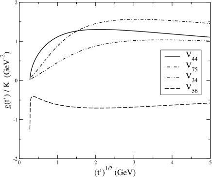
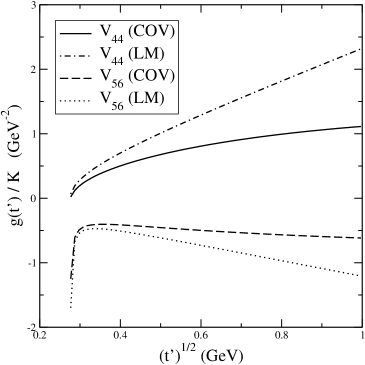
Figure 4: Spectral functions $g(t^{\prime})$ in units of GeV^-2, with the coefficient $\tilde{K}$ factored out, and represented as a function of $t^{\prime 1/2}$ to better emphasize the low-$t^{\prime}$ range. Left panel: for $t^{\prime 1/2}$ from threshold to $5\,{\rm GeV}$ for all functions, to show the relative importance of the various components and the beginning of the onset of the asymptotic behavior, $t^{\prime-1/2}$. Right panel: from threshold to $1\,{\rm GeV}$ for functions $g_{44}(t^{\prime})$ and $g_{56}(t^{\prime})$ together with their large-$M$ limits, to check the validity of this approximation.

We consider in this section various numerical aspects of the potentials presented in the previous one. They successively concern the spectral functions, $g_{ij}(t^{\prime})$, the potentials in momentum space, $v_{ij}(q)$, and the potentials in configuration space, $v_{ij}(r)$. In most cases, we directly compare the results of the covariant approach (COV) with those obtained from it in the large-$M$ limit (LM), Eqs. (20). This comparison is more meaningful than the one with the EFT potential (EFT), Eqs. (12), as it is not biased by the choice of the factor $\Lambda_{\chi}$ and by the difference of a factor $g_{A}$, instead of $g_{A}^{3}$, in part of the contribution to $V_{56}$, of which origin is understood in any case. Before entering into details, we notice that the various components of the interaction have a local character for some of them ($V_{44}$ and $V_{56}$) and a non-local one for the other ones ($V_{34}$ and $V_{75}$). At low energy, however, it turns out that one of the contributions involving the factor $\vec{p}$ or $\vec{p}\,^{\prime}$ in their expression, Eq. (7), is small. Moreover, with our conventions, the spin-isospin factors give the same values for the $z$ component. The various components can then be usefully compared, independently of their local or non-local character, that is what we do here. Numerical results assume the following values: $g_{\pi NN}=13.45,\;g_{A}=1.2695,\;M=938.919{\rm MeV},\;m_{\pi}=138.039{\rm MeV},\;m_{\rho}=771.1{\rm MeV}$.

         

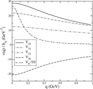
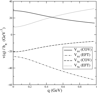
Figure 5: Potentials $v_{44}(q)$, $v_{34}(q)$, $v_{56}(q)$ and $v_{75}(q)$ (together with the OPE one divided by 10) for $q$ ranging from 0 to 1 GeV (left panel) and their EFT counterpart for $v_{44}(q)$ and $v_{56}(q)$ (right panel). Ingredients entering the EFT results are specified in the text. Notice that the EFT and “covariant” versions of a given component of the potential have opposite signs.

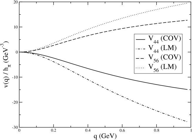
Figure 6: Subtracted potentials $v_{44}(q)$ and $v_{56}(q)$ for $q$ ranging from 0 to 1 GeV: comparison of the large-$M$ limit approach (LM, Eqs. (20)) with the covariant one. The asymptotic $q$ dependence of the “covariant” results is a constant one while the one for large-$M$ limit results has an extra ln$(q)$ dependence.

         

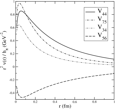
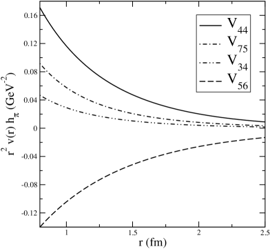
Figure 7: Potentials $v_{44}(r)$, $v_{34}(r)$, $v_{56}(r)$ and $v_{75}(r)$ at small and intermediate distances (left and right panels respectively). The results shown in the figure represent the above potentials multiplied by a phase factor, $r^{2}$ (in units of GeV^-2), to better emphasize the most relevant range for applications.

         

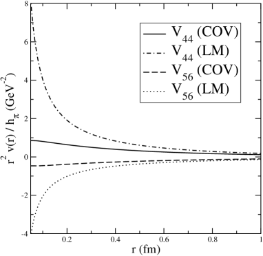
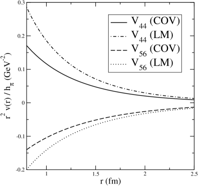
Figure 8: Potentials $v_{44}(r)$ and $v_{56}(r)$ at small and intermediate distances (left and right panels respectively): comparison of the “covariant” calculations with their large-$M$ limits; other definitions or comments as in Fig. 7. The curves corresponding to the large-$M$ limit in the left panel tend to $\infty$ when $r\rightarrow 0$ and have a zero-range part, not shown in the figure, with an opposite sign.

We begin with the first four spectral functions $g_{ij}(t^{\prime})$ entering potentials $V_{44}$, $V_{34}$, $V_{56}$ and $V_{75}$. Their $t^{\prime}$ dependence is shown for a range of $t^{\prime 1/2}$ going from threshold to about $5\,{\rm GeV}$ in Fig. 4 (left panel). It is aimed to roughly evidence the relative weight of various components at small and high $t^{\prime}$. At first sight, different potentials have comparable sizes. The small-$t^{\prime}$ range is physically more relevant in the sense that the regime beyond $1\,{\rm GeV}^{2}$ is expected to involve the contribution of other multi-meson exchanges. The higher-$t^{\prime}$ range is more appropriate to illustrate convergence properties. At low values of $t^{\prime}$, one can see some significant differences as expected from the $1/M$ expansion, Eq. (18). For $t^{\prime 1/2}\leq 0.5\,{\rm GeV}$, the spectral functions entering the local potentials, $V_{44}$ and $V_{56}$, dominate those of the non-local ones, $V_{34}$ and $V_{75}$. All of them increase in the lower-$t^{\prime}$ range (except in a very small $t^{\prime}$ range for $V_{56}$) and one has to go to much higher values of this variable to observe some saturation and ultimately some decrease. The maximum is roughly reached around $t^{\prime 1/2}\!=\!2M$, which, apart from the pion mass, is the only quantity entering the calculations. The decrease, roughly given by $t^{\prime-1/2}$, up to log terms, ensures good convergence properties for potentials $v_{ij}(q)$, Eq. (5) (this would not be the case for the other Green function mentioned in the text, see details in Appendix A.2). The validity of the $1/M$ expansion for the spectral functions $g_{44}(t^{\prime})$ and $g_{56}(t^{\prime})$, which allows one to recover the EFT results for the essential part, can be checked by examining Fig. 4 (right panel), where the “covariant” and approximate results are shown for a $t^{\prime}$ range extending to $1\,{\rm GeV}^{2}$. It is observed that the dominant term in the $1/M$ expansion tends to overestimate the more complete results both at very low and high values of $t^{\prime}$. In the first case, the threshold behavior ($q_{\pi}^{3}$ for $g_{44}(t^{\prime})$, arctg$(m^{2}_{\pi}/q_{\pi}M)$ for $g_{56}(t^{\prime})$) is missed (see observation on the $1/M$ expansion in the previous section). In the second case, the overestimation, which is roughly given by a factor $t^{\prime}/M^{2}$, tends to increase with $t^{\prime}$, preventing one from getting convergent results.

In Fig. 5 (left panel), we show the potentials $v_{ij}(q)$ up to $q\!=\!1$ GeV (together with the OPE one that has a strong dependence on $q$ and is divided by 10 to fit the figure). As expected from examination of the spectral functions, the TPE potentials have roughly the same size and there is no strong evidence that some of them should be more important than other ones. It is also noticed that their decrease in the range $q=$(0$-$1) GeV is slower than the standard $\rho$-exchange one, given by $1/(m_{\rho}^{2}\!+\!q^{2})$, indicating they roughly correspond to a shorter-range interaction. The comparison of the potentials, $v_{44}(q)$ and $v_{56}(q)$, with the corresponding EFT ones, Eqs. (12), can be made by looking at Fig. 5 (right panel). The choice of $\Lambda_{\chi}$ in the EFT results ($\Lambda_{\chi}=4\pi\,g_{A}\,M/g_{\pi NN}$) is suggested by the large-$M$ limit of the “covariant” expression, see Eqs. (20), to make the comparison as meaningful as possible. A striking feature appears here: the EFT potentials have a sign opposite to the “covariant” ones but the $q$ dependence is roughly the same. This feature suggests that the LEC part could play an important role.

To make a more significant comparison, we subtracted a constant from both potentials so that they vanish at $q^{2}\!=\!0$. This procedure amounts to using subtracted dispersion relations, which leads to convergence in all cases. Moreover, in configuration space, this part of the interaction determines the long-range component of the potential, which is physically the most relevant one. Results are shown in Fig. 6. The “covariant” and LM results have now the same sign. It is however noticed that the present LM results tend to overestimate the “covariant” ones. In the limit $q\rightarrow 0$, the overestimate reaches a factor 1.6 for $V_{44}$ and a factor 1.3 for $V_{56}$. This points in this case to the role of higher $1/M$-order corrections. Actually, the discrepancy vanishes in the limit $m_{\pi}/M\rightarrow 0$, showing that the non-zero pion mass has some effect. The discrepancy tends to slowly increase with $q$ (factors 1.9 and 1.5 at $q\!=\!$1 GeV for $V_{44}$ and $V_{56}$ respectively), pointing out to the role of ln($q$) corrections appearing in the large-$M$ limit. Altogether, these results are in accordance with the overestimate already noticed for spectral functions in this approximation. ¿From a different viewpoint, these results confirm the expectation that the discrepancy between the EFT and “covariant” approaches shown in the right panel of Fig. 5 can be ascribed to contact terms. A rough agreement would be obtained with the effective potential obtained in the $\overline{\mbox{\rm MS}}$ together with a dimensional-regularization scale $\mu$ ranging from $3\,m_{\pi}$ to $6\,m_{\pi}$, depending on how this is made (see the definition of this scheme at the end of Appendix B).

The Fourier transforms of the $v_{ij}(q)$ quantities, $v_{ij}(r)$, are shown in Fig. 7 for small distances (left panel) as well as intermediate distances (right panel). We call them potentials though they are dimensionless quantities, the energy dimension being given by the extra operators $\vec{p}$. They are multiplied by a factor $r^{2}$ to emphasize the range which is relevant in practice for calculations. At small distances, the comparison of various components roughly reflects the one for spectral functions or potentials in momentum space. Examination of these results at large distances evidences some significant differences. They have a better agreement with expectations from the $1/M$ expansion or from the very-low-$t^{\prime}$ behavior of spectral functions. Thus, the local potentials, $v_{44}(r)$ and $v_{56}(r)$, have a range larger than the other two components, $v_{34}(r)$ and $v_{75}(r)$, do. The differences appear only in the range where potentials have small contributions to PV effects.

The comparison with the LM potentials is given in Fig. 8 for the local components ($V_{44}$ and $V_{56}$). It is noticed that these last potentials should be completed by contact terms, which have a sign opposite to the corresponding curves. Due to the difficulty of representing these terms in a simple way, they have not been drawn in this figure. Moreover, they are not distinguishable from the LEC’s contributions and have thus an arbitrary character (they depend on the subtraction scheme). Considering first potentials at intermediate (or long) distances, where they can be the most reliably determined, it is found that the LM and “covariant” potentials have the same sign despite they have opposite sign in momentum space. This result is in complete accordance with the subtracted potentials shown in Fig. 6. Indeed, the slope of the corresponding results is, up to a minus sign, a direct measure of the square radius of the potential weighted by its strength. The negative slope for the potential $V_{44}$ thus indicates that its configuration-space representation is positive at intermediate distances (the opposite for $V_{56}$). Quantitatively, the significant dominance of the LM results over the “covariant” ones (factors 1.7 and 1.4 for $V_{44}$ and $V_{56}$ respectively at $r=0.8$ fm) confirms what is found for subtracted potentials in momentum space. Considering now the very short-range domain, it is found that the product of the LM potentials with $r^{2}$, which are shown in Fig. 8 (left panel), diverge like $1/r$ when $r\rightarrow 0$, up to log factors. The contribution of this part alone to the plane-wave Born amplitude is thus logarithmically divergent. This contribution turns out to be canceled by the zero-range one, mentioned above, so that the sum is finite. Thus, there is no principle difficulty with this peculiar behavior of the LM potentials in configuration space but, of course, some care is required in estimating their contribution.

         

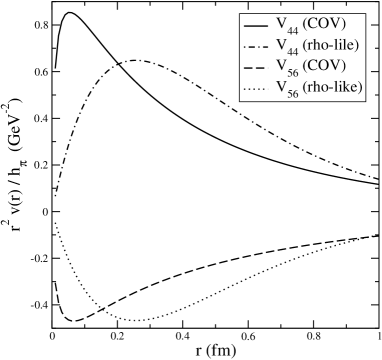
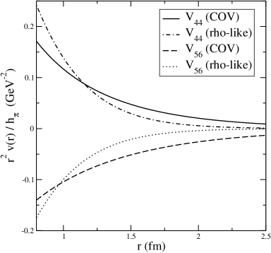
Figure 9: Potentials $v_{44}(r)$ and $v_{56}(r)$ at small and intermediate distances (left and right panels respectively): comparison of the “covariant” calculations with a standard rho-exchange potential normalized to the same volume integral; other definitions or comments as in Fig. 7.

Naively, it could be thought that the TPE is a medium-range interaction, as already mentioned. In Fig. 9, we compare potentials $v_{44}(r)$ and $v_{56}(r)$ to a standard rho-exchange one normalized so that they have the same volume integral. This quantity determines the low-energy plane-wave Born amplitude (up to a factor $\vec{p}$ which can be factored out). At very large distances, the effect of the longer-range TPE tail is evident but this occurs in a domain where the potential is quite small and will not contribute much. At intermediate or even at small distances however, the TPE roughly compares to the $\rho$ exchange. Actually, it turns out to have a shorter range. This reflects the fact that the two-pion continuum has an unlimited mass (the integration over $t^{\prime}$ extends to infinity). Moreover, it is slightly more singular at very small distances, as a result of the extra ln(r) dependence of the TPE potential. This last effect is typical of relativistic effects. Both long- and short-distance effects can be traced back to the $g(t^{\prime})$ function which, in the TPE case, extends to both small and large values of $t^{\prime}$ with a maximum around $t^{\prime}\!=\!4M^{2}$, while it is concentrated around $t^{\prime}\!=\!m^{2}_{\rho}$ for the $\rho$-exchange one ($\delta(t^{\prime}\!-\!m^{2}_{\rho})$ function in the zero-width limit).

For simplicity, we did not consider explicitly the contribution due to nucleon resonances in the two-pion box diagrams, which was accounted for in the 70’s in a “covariant” approach [15] or recently in a EFT [16, 17] or a TO one [18]. As already mentioned, part of it is contained in the EFT approach by relying on the Weinberg-Tomozawa description of the $\pi N$ scattering amplitude. It only contributes to the $V_{56}$ component and could represent 10$-$20% of the total contribution, depending on the range and how it is estimated. On top of it, there are further contributions which affect both $V_{44}$ and $V_{56}$ components. In the case of $V_{44}$, they amount to an extra 30$-$40% contribution around 1 fm in the “covariant” calculation [15] and roughly twice as much in the EFT approach [16, 17] or the TO one [18]. For the case of $V_{56}$, it is more complicated as the above mentioned contribution relative to the description of the $\pi N$ scattering amplitude has to be disentangled first for the “covariant” calculation. When this is done, the extra contribution due to resonances decreases and could represent 30$-$40% of the contribution with nucleons only [15]. This is slightly less than what is obtained in the EFT approach [16]. Taking into account that the EFT results overestimate the “covariant” ones for the nucleon intermediate state, it thus appears that the overestimate for the resonance intermediate state is significantly larger. This feature points to corrections of order $p^{2}/(M(M_{\Delta}\!-\!M))$ affecting the resonance propagator (dispersion effects), which are known to be important, while corrections in relation with the large-$M$ limit are of order $p^{2}/M^{2}$. It reinforces the conclusion of Ref. [16] that, contrary to the strong-interaction case, the role of resonances, especially the $\Delta(1232\;{\rm MeV})$ one, plays a negligible role in the PV $NN$ interaction.

6 Estimates of PV effects in two processes

The TPE potentials considered here have an isovector character. At low energy, they can contribute to two different transitions, ${}^{1}S_{0}\!-\!\!\,^{3}P_{0}$, which involves identical particles like two protons or two neutrons and ${}^{3}S_{1}\!-\!\!\,^{3}P_{1}$, which involves different particles, proton and neutron. The interactions $V_{44}$ and $V_{34}$ contribute in the first case while the interactions $V_{56}$ and $V_{75}$ contribute in the other one. Two processes of current interest, where the TPE potentials matter, are respectively proton-proton scattering and radiative neutron-proton capture at thermal energy. In the first case, a helicity dependence of the cross section, $A_{L}(E)$, has been measured at different energies [32, 33, 34]. In the second case, an asymmetry in the direction of the photon emission with respect to the neutron polarization, $A_{\gamma}$, has been looked for at LANSCE [35] (the experiment is now running at SNS). The TPE contribution to these effects is discussed in the following. The calculations have been performed with the $NN$-strong-interaction model, Av18 [36], which is local wave by wave. Vertex form factors are ignored. On the one hand, the dispersion-relation formalism assumes on-mass-shell particles, the contribution due to form factors in other approaches being generated by what is included in the dispersion relations. On the other hand, the role of form factors was already examined within the EFT approach [10, 11], partly with the motivation of regularizing a potential that is badly behaved at short distances, $\propto(r^{-3}\!-\!c\,\delta(\vec{r}\,))$ where $c$ is infinite and “determined” so that the integral over $\vec{r}$ has a well-defined value. There is no principle difficulty to work with this potential, however, and we will therefore use it here. This will facilitate the comparison with the “covariant” results.

As a side remark, we notice that form factors different from those mentioned above have been used in the context of applying effective field theories to the strong $NN$ interaction [4]. They involve a separable dependence of the relative momentum in the initial and final states, $\vec{p}$ and $\vec{p}\,^{\prime}$, instead of $\vec{q}=\vec{p}-\vec{p}\,^{\prime}$. Their effect is to smooth out wave functions at short distances in accordance with the idea that the corresponding physics, partly unknown, should be integrated out and accounted for by LEC’s. For such form factors, it would be more convenient to work in momentum space. However, in the case where configuration space is chosen, the methods we used for dealing with the badly-behaved potential could be useful there too.

6.1 Proton-proton scattering

The first calculation of TPE effects was done by Simonius [37], with the aim to get some estimate for a measurement of PV effects in $pp$ scattering (the Cabibbo model then used was not contributing to the $pp$ force in its simplest form). Our results, obtained here for three energies at which the longitudinal asymmetry $A_{L}(E)$ has been measured, are presented in Table 1.

Examining the “covariant” results, it is found that the contribution of the local term, $V_{44}({\rm COV})$, dominates over the non-local one, $V_{34}({\rm COV})$, which appears at the next order in the $1/M$ expansion. The result could be guessed from looking at Fig. 7. Their ratio is of the order of the factor $1+\mu_{V}=4.706$ which appears in the $\rho$-exchange potential. There are reasons to think this result is not accidental (see end of Sect. 4). The present results compare to the earlier ones [37] as well as with the value $A_{L}(13.6\,{\rm MeV})=-0.1\,h^{1}_{\pi}$ that has been used in analyses of PV effects [31]. The closeness can be attributed to the fact that the Av18 model employed here and the Reid or Hamada-Johnston models previously used are local ones and, moreover, evidence a strong short-range repulsion. Significant departures could occur, instead, with models like CD-Bonn [38] or some Nijmegen ones [39], which have a non-local character (see Ref. [40] for a discussion about the role of non-locality).

Table 1: PV asymmetries in $pp$ scattering at three energies, 13.6, 45 and 221 MeV: successively for the potentials $V_{44}({\rm COV})$, $V_{34}({\rm COV})$, $V_{44}({\rm rho}$-${\rm like})$ and $V_{44}({\rm LM})$, in units of the $h^{1}_{\pi}$ coupling constant.

Energy (MeV)	13.6	45	221
$V_{44}({\rm COV})$	-0.092	-0.154	0.072
$V_{34}({\rm COV})$	-0.022	-0.042	-0.029
$V_{44}({\rm rho}$-${\rm like})$	-0.110	-0.196	0.096
$V_{44}({\rm LM})$	-0.150	-0.252	0.127

Due to its long-range component, one could infer that the TPE contribution should be enhanced with respect to the $\rho$-exchange one when the effect of short-range repulsion is accounted for. The comparison of $V_{44}({\rm rho}$-${\rm like})$ and $V_{44}({\rm COV})$ results shows that this is the other way round. This can be explained by the fact that the long-range contribution where the TPE dominates over the $\rho$-exchange has little contribution to the asymmetry (a few %). Instead, the short-range contribution where the TPE dominates over the $\rho$-exchange plays a bigger role. The effect of short-range repulsion on this contribution will therefore be enhanced, hence decreasing of the total TPE contribution with respect to the $\rho$-exchange one.

6.2 Asymmetry in neutron-proton radiative capture

Contrary to $pp$ scattering discussed above, the asymmetry $A_{\gamma}$ involves a non-zero contribution from OPE. Thus, independently of the value of the coupling $h^{1}_{\pi}$, one can directly compare the TPE and OPE contributions. The last one has been extensively studied, see Ref. [41] and earlier references therein, and Refs. [10, 11, 42] for more recent works. Its contribution is approximately given by $A_{\gamma}(OPE)=-0.11h^{1}_{\pi}$ ($=-0.112h^{1}_{\pi}$ for the Av18 model used here).

The TPE contributions to $A_{\gamma}$ for the “covariant” case are given by:

$$A_{\gamma}(V_{56}({\rm COV}))=0.0093\,h^{1}_{\pi},$$

$$A_{\gamma}(V_{75}({\rm COV}))=-0.0040\,h^{1}_{\pi},$$ (22)

while those for the rho-like and large-$M$ limit are:

$$A_{\gamma}(V_{56}({\rm rho\!-\!like}))=0.0093\,h^{1}_{\pi},$$ (23)

$$A_{\gamma}(V_{56}({\rm LM}))=0.0141\,h^{1}_{\pi}.$$ (24)

Considering the “covariant” results, it is first noticed that the contribution of the local term, $V_{56}({\rm COV})$, dominates over the non-local one, $V_{75}({\rm COV})$, which appears at the next $1/M$ order. The effect is however less important than in $pp$ scattering, which can be inferred from looking at the corresponding potentials in Fig. 7. Moreover, contrary to this process, their contributions have opposite signs. Thus, the total contribution represents only $-$5% of the OPE one. This is good news in the sense that it confirms that the asymmetry $A_{\gamma}$ represents the best observable to determine the coupling $h^{1}_{\pi}$. Present results reasonably compare to an earlier one [19]: $A_{\gamma}(TPE)=0.008\,h^{1}_{\pi}$, which is added up by $A_{\gamma}(V_{56})=0.0107\,h^{1}_{\pi}$ and $A_{\gamma}(V_{75})=-0.0027\,h^{1}_{\pi}$. Part of the difference for $A_{\gamma}(V_{56})$ can be traced back to the omission here of the $\Delta$ resonance contribution in intermediate states. It is reminded that this contribution tends to make the $\pi N$-scattering amplitude consistent with the Weinberg-Tomozawa coupling, resulting in an enhancement of the $V_{56}$ interaction (see discussion in Sec. 4). The main difference for $A_{\gamma}(V_{75})$ is due to the extension of the integration over $t^{\prime}$ in the dispersion relation from $50\,m_{\pi}^{2}$ to $\infty$ here.

At first sight, the comparison of the TPE and $\rho$-exchange results, which are essentially the same, shows features different from those observed in $pp$ scattering. Examination of Fig. 9 indicates that, in comparison to the $V_{44}$ potential, the enhancement of the TPE potential, $V_{56}({\rm COV})$, over the $\rho$-exchange one, $V_{56}({\rm rho}$-${\rm like})$, is larger at large distances and smaller at short distances. As a result, the two effects due to the short-range repulsion mentioned for $pp$ scattering tend to cancel here.

6.3 Results in the large-$M$ limit

Involving the subtraction of an infinite term, results obtained in the large-$M$ limit, which can be identified with the EFT ones for the essential part, cannot be directly compared to the “covariant” ones. A first look nevertheless shows that the results, apart from an enhancement by a factor 1.5 or so, are very similar. Moreover, from considering the plane-wave Born approximation, we should have expected opposite signs. It is therefore appropriate to give some explanation helping to understand these results.

We first checked which range was contributing to PV asymmetries and found that the role of the range below 0.4$-$0.5 fm was rather small (10$-$20%). The observed enhancement of the large-$M$ result over the “covariant” one thus reflects the similar enhancement that can be inferred from the corresponding potentials in Fig. 8, around 0.8 fm. The little role of the range below 0.4$-$0.5 fm is not expected from considering Fig. 7. Instead, it can be related to the strong interaction model, Av18, used to calculate wave functions entering estimates of observables. This model evidences the effect of a strong repulsion at short distances. As this effect is much less pronounced with non-local models, one can expect that the use of models like CD-Bonn or some Nijmegen ones, will show some differences with the present results. We can anticipate an increase of the magnitude of the “covariant” results and a decrease of the LM ones (without excluding in this case a change in sign reminding that one for the plane-wave Born approximation).

While trying to understand the role of higher $1/M$-order corrections, we face the problem that the corresponding contributions to potentials are more singular than those for $V_{44}({\rm LM})$ or $V_{56}({\rm LM})$, requiring some regularization and introduction of further LEC’s. Restricting our study to the range $r\geq$ 0.4$-$0.5 fm, which provides most of the contribution to the PV asymmetries, we found that the contribution at the next $1/M$ order had a sign opposite to the dominant one, which it largely cancels in the range around 0.8 fm. The correction, which is larger than needed, suggests that other corrections are necessary to ensure reasonable convergence. Among them, one could involve chiral symmetry breaking. We checked that in the limit of a massless pion, the “covariant” potential $v_{44}(r)$ and its large-$M$ limit are significantly closer to each other. A non-zero pion mass could thus explain a sizable part of the discrepancy for observables between the “covariant” and the large-$M$-limit results. We notice that the comparison of the EFT and “covariant” approaches in the strong interaction case evidences features similar to the above ones (see Ref. [21] and references therein). As far as we can see, the similarity is founded for a part.

The large-$M$ limit of “covariant” potentials assumes a particular subtraction scheme. In another scheme, the $\overline{\mbox{\rm MS}}$ one, part of the functions $L(q)$ appearing in Eqs. (20) are replaced by $L(q)\!-\!1\!-\!{\rm ln}(\mu/m_{\pi})$ (see Appendix B). Due to the effect of short-range repulsion in the Av18 model, the correction has little effect on the calculated observables (a few % increase for the $S\!-\!P$ transition part). This would be different for non-local models where the correction could be significantly larger. Depending on the value of the parameter $\mu$, a large part of the sensitivity of the LM results to strong-interaction models mentioned above could be removed [10]. We notice that a discussion similar to the above one on the role of the subtraction scheme has also been held in the strong-interaction case [4]. It was concluded that the spectral function regularization scheme (SFR) was providing better convergence properties than for the dimensional-regularization one, due to avoiding spurious short-range contributions. To some extent, the SFR scheme is close to the $\overline{\mbox{\rm MS}}$ one considered here, with the parameter $\tilde{\Lambda}$ introduced in the former case being replaced by the quantity $2\mu$ in the latter case.

7 Conclusion

In the present work, we have compared different approaches for incorporating the two-pion-exchange contribution to the PV $NN$ interaction. They include a covariant one, which fully converges and can thus be considered as a benchmark, and an effective-field-theory and a time-ordered one which can contain infinities. The last two approaches involve two components at the leading order, with a local character, while the covariant one involves both local and non-local. For a given transition, one can thus compare the local components obtained from different approaches on the one hand, local and non-local components on the other hand. These two comparisons can allow one to assess how good is the assumption of dominant order in the effective-field theory approaches as well as the role ascribed to LEC’s.

We first notice that the effective-field theory (EFT) approach, the time-ordered-diagram approach and the limit of the covariant one at the lowest non-zero order in the $1/M$ expansion (LM) essentially agree with each other for the local terms. Possible discrepancies involve ingredients that have been omitted (contribution of baryon resonances in particular) but are unimportant for the comparison. We can thus concentrate on a comparison of the covariant approach with its LM limit. Taking into account that this approach is determined up to contact terms, rough agreement is found. This is better seen by considering the subtracted potentials in momentum space or intermediate distances ($r=1$fm) in configuration space. Quantitatively, the LM (EFT) approach tends to overestimate the “covariant” results. At low $q$ or at intermediate distances, the effect reaches factors 1.7 and 1.3 respectively for the transitions ${}^{1}S_{0}\!-\!\!\,^{3}P_{0}$ and ${}^{3}S_{1}\!-\!\!\,^{3}P_{1}$. At very small but finite distances, the LM (EFT) potentials become very singular and their contribution to physical processes diverge. This divergence is canceled by the contribution associated to the contact term so that the total result is finite (after renormalization). This peculiar behavior at $r=0$ and around contrasts with the smooth but diverging behavior in momentum space of the published EFT two-pion-exchange interaction. In this case, it turns out that the sign of the potential is opposite to that one at finite distances, which is the most relevant part. This suggests that this EFT two-pion-exchange potential is dominated by an unknown contact term, as far as a comparison with the “covariant” result is concerned. The problem disappears with a different subtraction scheme, like the minimal one with a dimensional-regularization scale $\mu$ in the range (3$-$6)$\,m_{\pi}$. This last choice tends to minimize the role of short distances, confirming the absence of a large sensitivity to cutoffs observed elsewhere [10]. Interestingly, the $\overline{\mbox{\rm MS}}$ scheme corresponds to cutting off the dispersion integrals at a value of $t^{\prime 1/2}$ around $2\mu$, which, together with the above value of $\mu$, is about (1$-$2) GeV. This is quite a reasonable value for separating the contribution of known physics from the unknown one to be integrated out. We thus believe that the choice of the $\overline{\mbox{\rm MS}}$ scheme would be more appropriate, the interaction then ascribed to the EFT two-pion-exchange one being a better representation of the most reliable part of the two-pion-exchange physics, which occurs at intermediate and large distances.

Comparing the non-local components to the local ones, it is found that they are rather suppressed at large distances. For such distances, the contribution to dispersion relations is expected to come from values of $t^{\prime}$ smaller than $M^{2}$. The suppression of non-local terms then reflects the fact that they have an extra $1/M$ factor in the $1/M$ expansion. At short distances, instead, the contribution to dispersion relations comes from large values of $t^{\prime}$. In this case, the local and non-local terms have the same $1/M$ order and they tend to have comparable contributions. Another aspect of the dependence on the range concerns the comparison with the $\rho$-meson exchange. Not surprisingly, the two-pion exchange dominates the $\rho$-meson exchange one at long distances but, the potential being relatively small there, not much effect is expected from this part on the calculation of observables. The two-pion-exchange contribution is slightly dominated by the $\rho$-meson exchange one at medium distances and dominates again the last one at very short distances. Taking into account that the dominant contributions come from short and intermediate distances, the two-pion-exchange contribution turns out to have a shorter range than the $\rho$-meson exchange.

We looked at the TPE contribution in two physical processes, $pp$ scattering and radiative thermal neutron-proton capture. Roughly, they confirm what could be inferred from examining potentials. The results from the “covariant” approach, calculated with the Av18 $NN$ strong-interaction model, essentially agree with earlier estimates based on other models. The main discrepancies evidence the role of some inputs such as the restriction on the $t^{\prime}$ value in the dispersion relations or the role of resonances in modeling the $\pi N$ scattering amplitude which enters these relations and we omitted here for simplicity. Despite plane-wave Born amplitudes calculated with the EFT two-pion-exchange and the “covariant” approaches have opposite signs, it turns out that their contributions to observables are relatively close to each other. This feature points to the Av18 model, which produces wave functions that evidence the effect of a strong repulsion at short distances. Such a property is interesting in that the main contribution to observables comes from intermediate and long distances, where the derivation of the TPE potential is the most reliable. It is thus found that the EFT two-pion-exchange at NNLO tends to overestimate the “covariant” results by about 50%, pointing to a non-negligible role of next order corrections. This is confirmed by the consideration of non-local terms, which correspond to higher-order terms. Their contribution is especially important in neutron-proton capture, due to a destructive interference with the dominant one. Thus, the result at the dominant $1/M$ order (LM) in this process exceeds the “covariant” one by a factor of about 2$-$3. Interestingly, present results are rather insensitive to the subtraction scheme as far as the coefficient, $1\!+\!{\rm ln}(\mu/m_{\pi})$, remains in the range of a few units. This is a consequence of the strong short-range repulsion present in the Av18 model. We however stress the fortunate character of this result. The use of non-local strong-interaction models, like CD-Bonn or some Nijmegen ones, could lead to different conclusions. Actually, far to be a problem, the dependences on the model expected for the contribution of the term $1\!+\!{\rm ln}(\mu/m_{\pi})$ and the EFT potential calculated in the maximal-subtraction (MX) scheme are likely to cancel for a large part.

By comparing different approaches to the description of the PV TPE $NN$ interaction, it was expected one could learn about their respective relevance. Implying a natural cutoff of the order of the nucleon mass, the “covariant” approach provides an unavoidable benchmark. This is of interest for the EFT approach which, up to now, has been considered at the lowest $1/M$ order. In improving this approach, a first step concerns the subtraction scheme. The minimal-subtraction one ($\overline{\mbox{\rm MS}}$), which involves a renormalization scale, $\mu$, is probably more favorable. By taking for this scale a value of the order of the nucleon mass (or the chiral-symmetry-breaking scale $\Lambda_{\chi}$), the scheme better matches the separation of the interaction into known and less known contributions, corresponding respectively to long and short distances. The LEC’s so obtained could be less dependent on the strong-interaction model. The next step should concern higher $1/M$-order terms, whose contributions are not negligible. This is likely to require a lot of work and caution, as the singular behavior of these terms at short distances increases with their order. Meanwhile, the “covariant” results could provide both a useful estimate and a relevant guide for their study.

Acknowledgments We thank the Institute for Nuclear Theory at the University of Washington for its hospitality and the Department of Energy for partial support during the completion of this work. The work of CHH was supported by the Korea Research Foundation Grant funded by the Korean Government (MOEHRD, Basic Research Promotion Fund) (KRF-2007-313-C00178). The work of SA was supported by the Korea Research Foundation and the Korean Federation of Science and Technology funded by the Korean Government (MOEHRD, Basic Research Promotion Fund) and SFTC grant number PP/F000488/1. The work of CPL was supported in part by the U.S. Department of Energy under contract DE-AC52-06NA25396. We are grateful to Prof. U. van Kolck for pointing out an inconsistency of the simplest time-ordered-diagram approach with chiral-symmetry expectations.

Appendix A Subtraction of the iterated OPE and related questions

A.1 Expressions of the spectral functions, $g(t^{\prime})$

Historically, the derivation of the isovector PV two-pion exchange started with the calculation of the crossed diagram [12]. The calculation of the non-crossed diagram, which implies the removing of the iterated OPE contribution and thus requires more care, came slightly later [13]. Last works along the same lines [14, 15] considered the two types of diagrams on the same footing. We first remind here some results relative to the crossed and non-crossed diagrams with the notations of Ref. [13] (functions $g_{A}(t^{\prime})$, $g_{B}(t^{\prime})$, $g_{C}(t^{\prime})$ and $g_{D}(t^{\prime})$, $g_{E}(t^{\prime})$ respectively). The functions $g_{A}(t^{\prime})$ and $g_{D}(t^{\prime})$ correspond to the same spin-isospin structure. The two versions of the iterated OPE discussed in the text, which concern the $g_{D}(t^{\prime})$ and $g_{E}(t^{\prime})$ functions, are considered. The one employed in Ref. [13] corresponds to the term with the factor $(E+M)$ in the integrand while the other one considered in later works contains the factor $2E$. The expressions read:

$$g_{A}(t^{\prime}) = \frac{1}{2M}\Bigg{(}\frac{G}{x}-\frac{H\;x}{x^{2}+4M^{2}q_{\pi}^{2}}\Bigg{)}\,,$$

$$g_{B}(t^{\prime}) = \frac{x}{M^{2}}\;g_{A}(t^{\prime})\,,$$

$$g_{C}(t^{\prime}) = \frac{1}{2M}\Bigg{(}\frac{4q_{\pi}}{\chi^{2}}+\frac{H}{M^{2}}-G\Big{(}\frac{1}{M^{2}}+\frac{1}{\chi^{2}}\Big{)}\Bigg{)}\,,$$

$$g_{D}(t^{\prime}) = -\frac{x}{M^{2}\;m^{2}_{\pi}}\;{\rm arctg}\Big{(}\frac{m^{2}_{\pi}}{2Mq_{\pi}}\Big{)}-\frac{G}{2xM}$$

$$+\int_{k_{-}^{2}}^{{k_{+}^{2}}}\frac{dk^{2}}{k^{2}\sqrt{k^{2}t^{\prime}\!-\!(m^{2}_{\pi}\!+\!k^{2})^{2}}}\Bigg{(}\frac{2E\,{\rm or}\;(E\!+\!M)}{E^{2}}\Big{(}\frac{k^{2}\!-\!x}{4M}\!-\!\frac{E\!-\!M}{2}\Big{)}\!+\!\frac{x}{2M^{2}}\Bigg{)}\,,$$

$$g_{E}(t^{\prime}) = \frac{4x^{2}}{M^{2}\,m^{2}_{\pi}\,t^{\prime}}\;{\rm arctg}\Big{(}\frac{m^{2}_{\pi}}{2Mq_{\pi}}\Big{)}+\frac{2G}{Mt^{\prime}}$$

$$\!\!+\int_{k_{-}^{2}}^{{k_{+}^{2}}}\frac{dk^{2}}{k^{2}\sqrt{k^{2}t^{\prime}\!-\!(m^{2}_{\pi}\!+\!k^{2})^{2}}}$$

$$\times\Bigg{(}\frac{2E\,{\rm or}\;(E\!+\!M)}{E^{2}}\Big{(}\frac{(k^{2}\!-\!x)^{2}}{Mt^{\prime}}\!-\!\frac{2(E\!-\!M)(k^{2}\!-\!x)}{t^{\prime}}\!+\!\frac{(E\!-\!M)^{2}}{M}\Big{)}\!-\!\frac{2x^{2}}{M^{2}t^{\prime}}\Bigg{)}\,,$$

where the various functions, $q_{\pi},\;x,\;\chi,\;G,\;H$, are given in the text, Eq. (10). The writing slightly differs from Ref. [13]. No non-relativistic approximation is made for the integrands. Moreover, the original term, ${\rm arctg}(2Mq_{\pi}/m^{2}_{\pi})/m^{2}_{\pi}$, has been transformed into $(\pi/2-{\rm arctg}(m^{2}_{\pi}/2Mq_{\pi}))/m^{2}_{\pi}$ and the factor $\pi/2/m^{2}_{\pi}$ has been inserted in the integral using the relation $\int_{k_{-}^{2}}^{{k_{+}^{2}}}dk^{2}/\Big{(}k^{2}\sqrt{k^{2}t^{\prime}\!-\!(m^{2}_{\pi}\!+\!k^{2})^{2}}\;\Big{)}=\pi/m^{2}_{\pi}$. With this rearrangement, it can be checked that the integrand has no singularity at $k^{2}=0$.

The $g(t^{\prime})$ functions considered in the present work are related to the above ones by the relations:

$$g_{44}(t^{\prime}) = \tilde{K}\,g_{C}(t^{\prime})\,,$$

$$g_{34}(t^{\prime}) = \tilde{K}\,g_{B}(t^{\prime})\,,$$

$$g_{56}(t^{\prime}) = \tilde{K}\,(g_{A}(t^{\prime})+g_{D}(t^{\prime}))\,,$$

$$g_{75}(t^{\prime}) = \tilde{K}\,g_{E}(t^{\prime})\,,$$ (26)

where $\tilde{K}$ is an overall constant given in Eq. (10). An important point to note is that the contributions of the term $G/2xM$ in $g_{A}(t^{\prime})$ and $g_{D}(t^{\prime})$, which dominate at low energy, exactly cancel. This cancellation is important in restoring the crossing symmetry for pions, a property that is fulfilled by the effective pion-nucleon interaction introduced in the EFT approach (triangle diagram).

A.2 Asymptotic behavior of the $g(t^{\prime})$ functions

The asymptotic behavior of the spectral functions $g_{44}(t^{\prime})$ and $g_{34}(t^{\prime})$, which only involve the crossed-diagram contribution, can be easily obtained from their expressions, Eqs. (9). The dominant term is of the order $1/(M\sqrt{t^{\prime}})$ up to some log factors, see Eq. (11). The asymptotic behavior of the two other spectral functions, $g_{56}(t^{\prime})$ and $g_{75}(t^{\prime})$, is considerably more complicated. Their analytic part contains terms with the behavior $-\tilde{K}\sqrt{t^{\prime}}/2M^{3}$ and $\tilde{K}\sqrt{t^{\prime}}/M^{3}$ respectively while the integral part requires careful examination.

The dominant term in the integral is given by the part proportional to $x$ and $x^{2}$ in the integrands of $g_{56}(t^{\prime})$ and $g_{75}(t^{\prime})$ respectively. As the integrands are the same up to a factor $-4x/t^{\prime}$, it is sufficient to consider the first case. Its contribution becomes:

$$I_{56} = -\tilde{K}x\int_{k_{-}^{2}}^{{k_{+}^{2}}}\frac{dk^{2}}{k^{2}\sqrt{k^{2}t^{\prime}\!-\!(m_{\pi}^{2}\!+\!k^{2})^{2}}}\Bigg{(}\frac{2E\;({\rm or}\;E+M)}{4M\,E^{2}}\!-\!\frac{1}{2M^{2}}\Bigg{)}$$ (27)

$$= \tilde{K}x\int_{k_{-}^{2}}^{{k_{+}^{2}}}\frac{dk^{2}}{k^{2}\sqrt{k^{2}t^{\prime}\!-\!(m_{\pi}^{2}\!+\!k^{2})^{2}}}\Bigg{(}\frac{(E\!-\!M)}{2M^{2}\;E}\Big{(}{\rm or}\;\frac{(E\!-\!M)(2E+M)}{4M^{2}\;E^{2}}\Big{)}\Bigg{)}$$

$$= \tilde{K}x\int_{k_{-}^{2}}^{{k_{+}^{2}}}\frac{dk^{2}}{\sqrt{k^{2}t^{\prime}\!-\!(m_{\pi}^{2}\!+\!k^{2})^{2}}}\Bigg{(}\frac{1}{2M^{2}\,E\,(E\!+\!M)}\Big{(}{\rm or}\;\frac{(2E+M)}{4M^{2}\;E^{2}(E\!+\!M)}\Big{)}\Bigg{)}\,,$$

where the first case corresponds to the quadratic-energy dependent Green’s function retained here and the second case to the linear one. After some algebra, it is found that in the large-$t^{\prime}$ limit and a negligible pion mass, the integral with the first integrand writes:

$$I_{56}(t^{\prime}\rightarrow\infty) \!\!\simeq\!\! -\frac{1}{2}I_{75}(t^{\prime}\rightarrow\infty)\simeq\frac{\tilde{K}}{M\sqrt{t^{\prime}}}\Bigg{(}\frac{t^{\prime}}{2M^{2}}-\frac{1}{8}\,{\rm ln}\Big{(}\frac{t^{\prime}}{M^{2}}\Big{)}+\frac{1}{8}-\frac{1}{2}\,{\rm ln}(2)\Bigg{)}\,.$$ (28)

The absence of the intermediate term $1/(M^{2})$ results from a non-trivial cancellation. All the other terms not considered here behave like $1/(M\sqrt{t^{\prime}})$ (up to log terms) for the most important ones. It can thus be checked that the contributions of order $\sqrt{t^{\prime}}/M^{3}$ to the spectral functions $g_{56}(t^{\prime})$ and $g_{75}(t^{\prime})$ cancel, leaving contributions of order $1/(M\sqrt{t^{\prime}})$.

Have we used the other Green’s function, the dominant contribution resulting from performing the integral would read:

$$I_{56}(t^{\prime}\rightarrow\infty) \!\!\simeq\!\! -\frac{1}{2}I_{75}(t^{\prime}\rightarrow\infty)\simeq\tilde{K}\frac{\sqrt{t^{\prime}}}{2M^{3}}\;\frac{2+\pi}{4}\,,$$ (29)

while the corresponding $g(t^{\prime})$ functions would be given by:

$$g_{56}(t^{\prime}\rightarrow\infty) \!\!\simeq\!\! -\frac{1}{2}g_{75}(t^{\prime}\rightarrow\infty)\simeq\tilde{K}\frac{\sqrt{t^{\prime}}}{2M^{3}}\;\frac{\pi-2}{4}\,.$$ (30)

Thus, contrary to the quadratic-energy dependent Green’s function, no cancellation of the dominant terms is found with the consequence that the dispersion integrals involving the spectral functions $g_{56}(t^{\prime})$ and $g_{75}(t^{\prime})$, Eqs. (5), do not converge (logarithmic divergence). Moreover, these functions evidence a sign change around $t^{\prime}=$(20$-$25)$\,{\rm GeV}^{2}$. Actually, this has little effect on the spectral functions at low values of $t^{\prime}$ but, of course, this prevents one from getting convergent results. The sensitivity of the configuration-space potentials was not exceeding 10% at $r=1$ fm [15].

Appendix B $PV$ two-pion exchange $NN$ potential from EFT

In this Appendix, we give the detail of the momentum-space contributions from the two-pion exchange diagrams shown in Fig. 2, employing heavy-baryon chiral Lagrangian and the dimensional regularization in the $d$-dimensional space-time, $d=4-2\epsilon$.

¿From the diagram (b), (c) and (d), we get:

$$V_{(b)} \!=\! -i(\vec{\tau}_{1}\times\vec{\tau}_{2})^{z}(\vec{\sigma}_{1}\!+\!\vec{\sigma}_{2})\!\cdot\!\vec{q}\,\frac{\pi g_{A}h_{\pi}^{1}}{\sqrt{2}(4\pi f_{\pi})^{3}}$$ (31)

$$\hskip 56.9055pt\times\left[\frac{1}{\epsilon}-\gamma+{\rm ln}(4\pi)+{\rm ln}\left(\frac{\mu^{2}}{m_{\pi}^{2}}\right)+2-2L(q)\right]\,,$$

$$V_{(c)} \!=\! -i(\vec{\tau}_{1}+\vec{\tau}_{2})^{z}(\vec{\sigma}_{1}\times\vec{\sigma}_{2})\!\cdot\!\vec{q}\,\frac{2\sqrt{2}\pi g_{A}^{3}h_{\pi}^{1}}{(4\pi f_{\pi})^{3}}\left[\frac{1}{\epsilon}-\gamma+{\rm ln}(4\pi)+{\rm ln}\left(\frac{\mu^{2}}{m_{\pi}^{2}}\right)+2-2L(q)\right]$$ (32)

$$-i(\vec{\tau}_{1}\times\vec{\tau}_{2})^{z}(\vec{\sigma}_{1}\!+\!\vec{\sigma}_{2})\!\cdot\!\vec{q}\,\frac{\sqrt{2}\pi g_{A}^{3}h_{\pi}^{1}}{2(4\pi f_{\pi})^{3}}$$

$$\hskip 56.9055pt\times\left\{-\frac{3}{2}\left[\frac{1}{\epsilon}-\gamma+{\rm ln}(4\pi)+{\rm ln}\left(\frac{\mu^{2}}{m_{\pi}^{2}}\right)+\frac{4}{3}\right]+3L(q)-H(q)\right\}\,,$$

$$V_{(d)} \!=\! -i(\vec{\tau}_{1}\times\vec{\tau}_{2})^{z}(\vec{\sigma}_{1}\!+\!\vec{\sigma}_{2})\!\cdot\!\vec{q}\,\frac{\sqrt{2}\pi g_{A}^{3}h_{\pi}^{1}}{2(4\pi f_{\pi})^{3}}$$ (33)

$$\hskip 56.9055pt\times\left\{-\frac{3}{2}\left[\frac{1}{\epsilon}-\gamma+{\rm ln}(4\pi)+{\rm ln}\left(\frac{\mu^{2}}{m_{\pi}^{2}}\right)+\frac{4}{3}\right]+3L(q)-H(q)\right\}\,,$$

where $L(q)$ and $H(q)$ are defined in Eq. (13), and the Euler number is given by $\gamma=0.5772\cdots$. The quantity $\mu$ represents the scale of the dimensional regularization, and $q=|\vec{q}\,|$ with $\vec{q}$ defined by Eq. (2). We note that we have employed, in the calculation of the diagram (d), the same prescription to subtract the two-nucleon-pole contribution as in Ref. [6], Eq. (C.3) .

All these potentials from the loop diagrams have infinities, i.e., the $1/\epsilon$ terms. Along with the finite constant terms, they are renormalized by the counter terms (PV $NN$ contact terms) $\tilde{C}_{2}+\tilde{C}_{4}$ and $C_{6}$ (see Eq. (5) in Ref. [6]). In the maximal-subtraction scheme (MX), the $L(q)$ and $H(q)$ terms, which are the only ones to contribute to the finite-range potential, are retained. This procedure fixes the associated contact term. In the minimal-subtraction scheme ($\overline{\mbox{\rm MS}}$), besides $L(q)$ and $H(q)$ terms, an extra term ${\rm ln}\Big{(}\mu^{2}/m_{\pi}^{2}\Big{)}+2$ (rather written as $2(1\!+\!{\rm ln}(\mu/m_{\pi}))$ in the main text), which produces a contact term, appears.

References

- [1] C. Ordoñez, L. Ray and U. van Kolck, Phys. Rev. C 53, 2086 (1996).
- [2] E. Epelbaum, W. Glöckle and U.-G. Meißner, Nucl. Phys. A 671, 295 (2000).
- [3] D. R. Entem and R. Machleidt, Phys. Rev. C 68, 04001 (2003).
- [4] For a recent review, see, e.g., E. Epelbaum, Prog. Part. Nucl. Phys. 57, 654 (2006), and references therein.
- [5] S. Weinberg, Phys. Lett. B 251, 288 (1990); Nucl. Phys. B 363, 3 (1991).
- [6] S.-L. Zhu, C. M. Maekawa, B. R. Holstein, M. J. Ramsey-Musolf and U. van Kolck, Nucl. Phys. A 748, 435 (2005).
- [7] G. S. Danilov, Sov. J. Nucl. Phys. 14, 935 (1972).
- [8] J. Missimer, Phys. Rev. C 14, 347 (1976).
- [9] B. Desplanques and J. Missimer, Nucl. Phys. A 300, 286 (1978).
- [10] C. H. Hyun, S. Ando and B. Desplanques, Phys. Lett. B 651, 257 (2007), nucl-th/0611018.
- [11] C.-P. Liu, Phys. Rev. C 75, 065501 (2007).
- [12] D. Pignon, Phys. Lett. 35B, 163 (1971).
- [13] B. Desplanques, Phys. Lett. 41B, 461 (1972).
- [14] H. Pirner and D. O. Riska, Phys. Lett. 44B, 151 (1973).
- [15] M. Chemtob and B. Desplanques, Nucl. Phys. B78, 139 (1974).
- [16] N. Kaiser, Phys. Rev. C 76, 047001 (2007).
- [17] Y.-R. Liu and S.-L. Zhu, nucl-th/0711.3838.
- [18] J. A. Niskanen, T. M. Partanen and M. J. Iqbal, nucl-th/0712.2399.
- [19] B. Desplanques, Nucl. Phys. A 242, 423 (1975).
- [20] C. H. Hyun, B. Desplanques, S. Ando and C.-P. Liu, nucl-th/0802.1606.
- [21] R. Higa, M. R. Robilotta and C. A. da Rocha, Nucl. Phys. A 790, 384 (2007).
- [22] S. Ando and H. Fearing, Phys. Rev. D 75, 014025 (2007).
- [23] A. Amghar, B. Desplanques and L. Theußl, Nucl. Phys. A 714, 213 (2003).
- [24] S. A. Coon and J. L. Friar, Phys. Rev. C 34, 1060 (1986).
- [25] M. Lacombe et al., Phys. Rev. C 21, 861 (1980).
- [26] G. Barton, Nuovo Cimento 19, 512 (1961).
- [27] S. L. Adler, Phys. Rev. 140, B736 (1965), W. I. Weisberger, Phys. Rev. 143, 1302 (1966).
- [28] B. Desplanques, J. F. Donoghue and B. R. Holstein, Ann. Phys. (N.Y.) 124, 449 (1980).
- [29] B. R. Holstein, Phys. Rev. D 23, 1618 (1981).
- [30] N. Kaiser and U.-G. Meissner, Nucl. Phys. A 499, 727 (1989).
- [31] B. Desplanques, Phys. Rep. 297, 1 (1998).
- [32] S. Kistryn et al., Phys. Rev. Lett. 58, 1616 (1987).
- [33] P. D. Eversheim et al., Phys. Lett. B 256, 11 (1991).
- [34] A. R. Berdoz et al., Phys. Rev. Lett. 87, 272301 (2001).
- [35] J. S. Nico and W. M. Snow, Ann. Rev. Nucl. Part. Sci. 55, 27 (2005).
- [36] R. B. Wiringa, V. G. J. Stoks and R. Schiavilla, Phys. Rev. C 51, 38 (1995).
- [37] M. Simonius, Phys. Lett. 41B , 415 (1972), Nucl. Phys. A 220, 269 (1974).
- [38] R. Machleidt, Phys. Rev. C 63, 024001 (2001).
- [39] V. G. J. Stoks et al., Phys. Rev. C 49, 2950 (1994).
- [40] A. Amghar and B. Desplanques, Nucl. Phys. A 714, 502 (2003).
- [41] B. Desplanques, Phys. Lett. B 512, 305 (2001).
- [42] C. H. Hyun, T.-S. Park and D.-P. Min, Phys. Lett. B 516, 321 (2001).