Two-cover descent on hyperelliptic curves

Abstract.

We describe an algorithm that determines a set of unramified covers of a given hyperelliptic curve, with the property that any rational point will lift to one of the covers. In particular, if the algorithm returns an empty set, then the hyperelliptic curve has no rational points. This provides a relatively efficiently tested criterion for solvability of hyperelliptic curves. We also discuss applications of this algorithm to curves of genus $1$ and to curves with rational points.

1. Introduction

In this paper we consider the problem of deciding whether an algebraic curve $C$ over a number field $k$ has any $k$-rational points. We assume that $C$ is complete and non-singular. A necessary condition for $C(k)$ to be non-empty is that $C$ has a rational point over every extension of $k$. In particular, for any place $v$ of $k$, the curve $C$ should have a rational point over the completion $k_{v}$ of $k$ at $v$.

For curves of genus $0$, this is sufficient as well: if a genus $0$ curve $C$ has a rational point over every completion $k_{v}$ of $k$, then $C(k)$ is non-empty. A $k_{v}$-point of $C$ is referred to as a local point of $C$ at $v$ and a $k$-point of $C$ is called a global point. For a genus $0$ curve $C$, having a local point everywhere (at all places of $k$) implies having a global point. Genus $0$ curves are said to obey the local-to-global principle for points.

The local-to-global principle is important from a computational point of view. One can decide in finite time whether a curve has points everywhere locally: for any curve $C$ over a number field $k$, the set $C(k_{v})$ is nonempty for all places $v$ outside an explicitly determinable finite set $S$. For the remaining places $v\in S$, one can decide in finite time if $C(k_{v})$ is non-empty as well. See [bruin:ternary] for some algorithms, in particular a quite efficient algorithm for hyperelliptic curves. Thus, whether a curve has points everywhere locally can actually be decided in finite time.

It is well known that curves of genus greater than $0$ do not always obey the local-to-global principle. Most proofs of this phenomenon are based on the fact that curves of positive genus can have unramified Galois-covers. In fact, if a curve $C$ of positive genus has a rational point $P$, then the Abel-Jacobi map allows us to consider $C$ as a non-singular subvariety of its Jacobian variety $\mathrm{Jac}(C)$. Since the map $\pi:\mathrm{Jac}(C)\to\mathrm{Jac}(C),Q\mapsto nQ+P$ is unramified, the pull-back $\pi^{*}(C)$ yields an unramified cover of $C$ that has a rational point mapping to $P$. More generally, an $n$-cover of $C$ is a cover that is isomorphic to one of this form over an algebraic closure $\overline{k}$ of $k$. Thus, if one can show that an algebraic curve $C$ does not have $n$-covers that have a rational point, then it follows that $C$ has no rational points. Even though $C$ may have points everywhere locally, it is possible that on every cover, rational points can be ruled out by local conditions.

The major content of this paper is inspired by the following well-known observation. Let $\phi:D\to C$ be an unramified cover of a curve $C$ over a number field $k$ that is Galois over an algebraic closure $\overline{k}$ of $k$. It is a standard fact, going back to Chevalley and Weil [chevweil:covers] that there is a finite collection of twists $\phi_{\delta}:D_{\delta}\to C$ of the given cover $\phi$ such that any rational point on $C$ has a rational pre-image on one of the covers $D_{\delta}$. We call such a set of covers a covering collection. Furthermore, at least in principle, such a finite collection of covers is explicitly computable given a cover $\phi:D\to C$.

Thus, one approach for testing solvability of a curve $C$ that has points everywhere locally is:

1. Fix $n\geq 2$.

2. Construct an $n$-cover $D$ of $C$. If no such covers exist, then $C(k)$ is empty.

3. Determine a covering collection associated to $D\to C$.

4. Test each member of the covering collection for local solvability. If none of the members has points everywhere locally then no curve in the covering collection has any rational points, and $C$ has no rational points either.

Each of the covers might have a local obstruction to having rational points, while the underlying curve $C$ has none. Thus the procedure sketched above can actually prove that a curve does not obey the local-to-global principle for points. See [stoll:covers] for a detailed discussion, including the theoretical background and some links to the Brauer-Manin obstruction against rational points.

In the present article we discuss a relatively efficient way of carrying out the procedure sketched above for hyperelliptic curves. We consider unramified covers $D/C$ over $k$ such that for an algebraic closure $\overline{k}$ of $k$ we have that $\mathrm{Aut}_{\overline{k}}(D/C)\simeq\mathrm{Jac}(C)[2](\overline{k})$ as $\mathrm{Gal}(\overline{k}/k)$-modules. These are exactly the two-covers of $C$ over $k$. We write $\mathrm{Cov}^{(2)}(C/k)$ for the set of isomorphism classes of two-covers of $C$ over $k$.

Our claim to efficiency stems from the fact that we avoid explicitly constructing a covering collection. In fact, the method can be described without any reference to unramified covers, see Section 2. Instead, we determine an abstract object that (almost) classifies the isomorphism classes of two-covers. See Section 3 for how to construct the covers explicitly from the information provided by the algorithm.

We observe that for any field extension $L/k$ there is a well-defined map $C(L)\to\mathrm{Cov}^{(2)}(C/L)$ by sending a point to the two-cover that has an $L$-rational point above it. For completions $k_{v}/k$, we show that this map is locally constant: If two points $P_{1},P_{2}\in C(k_{v})$ lie sufficiently close, then they lift to the same two-cover. This allows us to explicitly compute the $k_{v}$-isomorphism classes of two-covers that have points locally at $v$. We can then piece together this information to obtain the global isomorphism classes of two-covers that have points everywhere locally.

We define $\mathrm{Sel}^{(2)}(C/k)\subset\mathrm{Cov}^{(2)}(C/k)$ to be the set of everywhere locally solvable two-covers of $C$. The algorithm computes a related object, that we denote by $\mathrm{Sel}_{\mathrm{fake}}^{(2)}(C/k)$, which is a quotient of $\mathrm{Sel}^{(2)}(C/k)$. It classifies everywhere locally solvable two-covers, up to an easily understood equivalence. Since any curve $C$ with a rational point admits a globally and hence everywhere locally solvable two-cover, $\mathrm{Sel}_{\mathrm{fake}}^{(2)}(C/k)=\emptyset$ implies that $C(k)$ is empty.

A priori, the elements of $\mathrm{Sel}_{\mathrm{fake}}^{(2)}(C/k)$ represent two-covers that have a model of a certain form (described in Section 3), but we will prove that every two-cover that has points everywhere locally does have such a model, see Theorem 3.4 below.

In Section 7 we illustrate how the algorithm presented in Sections 4, 5, and 6 can be used to show that a hyperelliptic curve has no rational points. This method was also used in a large scale project [brusto:smallgenus2] to determine the solvability of all genus $2$ curves with a model of the form

$$y^{2}=f_{6}x^{6}+\cdots+f_{0},\mbox{\quad where }f_{i}\in\{-3,-2,-1,0,1,2,3\}\mbox{ for }i=0,\ldots,6.$$

In Section 10 we describe some statistics that illustrate how frequently one would expect that $\mathrm{Sel}_{\mathrm{fake}}^{(2)}(C/k)=\emptyset$ for curves of genus $2$.

Section 8 shows how information obtained on $\mathrm{Sel}_{\mathrm{fake}}^{(2)}(C/k)$ can be used for determining the rational points on curves if $C(k)$ is non-empty. This complements Chabauty-methods as described in [bruintract, bruin:ellchab, flynnweth:biell]. In earlier articles, the selection of the covers requiring further attention was done by ad-hoc methods. Here we describe a systematic and relatively efficient approach.

In Section 9 we describe the results of applying the method to curves of genus $1$. We find (unsurprisingly) that we recover well-known algorithms for performing $2$-descents and second $2$-descents on elliptic curves [cassels:lecec, mss:seconddesc]. A practical benefit of this observation is that to our knowledge, nobody has bothered to implement second two-descent over arbitrary number fields, whereas our implementation in MAGMA [magma] (which is available for download at [brusto:implementation]) can immediately be used. We give an example by exhibiting an elliptic curve over $\mathbb{Q}(\sqrt{2})$ with a non-trivial Tate-Shafarevich group.

2. Definition of the fake $2$-Selmer group

Let $k$ be a field of characteristic $0$ and let $C$ be a non-singular projective hyperelliptic curve of genus $g$ over $k$, given by the affine model

$$C:y^{2}=f_{n}x^{n}+\cdots+f_{0}=f(x),\mbox{\quad where $f$ is square-free}.$$

If $n$ can be chosen to be odd, then $C$ has a rational Weierstrass point. This is a special situation and, by not placing any Weierstrass point over $x=\infty$, we see that we lose no generality by assuming that $n$ is even, in which case $n=2g+2$. In practice, however, computations become considerably easier by taking $n$ odd if possible. The construction below can be adapted to accommodate for odd $n$. See Remark 2.1 below.

From here on we assume that $n$ is even unless explicitly stated otherwise. We consider the algebra

$$A=k[x]/(f(x))$$

and we write $\theta$ for the image of $x$ in $A$, so that $f(\theta)=0$. We consider the subset of $A^{*}$ modulo squares and scalars (elements of $k^{*}$) with representatives in $A^{*}$ that have a norm in $k^{*}$ that is equal to $f_{n}$ modulo squares:

$$H_{k}=\{\delta\in A^{*}/A^{*2}k^{*}:N_{A/k}(\delta)\in f_{n}k^{*2}\}.$$

The set $H_{k}$ might be empty (but see Question 7.2). As we will see, this implies that $C$ has no rational points. This follows from the fact that we can define a map $C(k)\to H_{k}$. First, we define the partial map:

$$\begin{array}[]{cccc}\mu_{k}:&C(k)&\to&H_{k}\\ &(x,y)&\mapsto&x-\theta\,.\end{array}$$

Here and in the following, we write $x-\theta$ instead of the correct, but pedantic, $(x-\theta)A^{*2}k^{*}$; we hope that no confusion will result. This definition of $\mu$ does not provide a valid image for any point $(x_{1},0)\in C(k)$. For any such point, we can write $f(x)=(x-x_{1})\tilde{f}(x)$ and we define:

$$\mu_{k}((x_{1},0))=(x_{1}-\theta)+\tilde{f}(\theta).$$

Furthermore, if $f_{n}\in k^{*2}$ then the desingularisation of $C$ has two points, say $\infty^{+},\infty^{-}$ above $x=\infty$. We define

$$\mu(\infty^{+})=\mu(\infty^{-})=f_{n},$$

where $f_{n}\equiv 1$ modulo $k^{*2}$.

Remark 2.1.

While we lose no generality by assuming that $f(x)$ is of even degree, for computational purposes it is often preferable to work with odd degree $f(x)$ as well. We can use the definitions above if we replace the definition of $H_{k}$ by

$$H_{k}=\{\delta\in A^{*}/A^{*2}:N_{A/k}(\delta)\in f_{n}k^{*2}\}.$$

In this case, there is a unique point $\infty$ above $x=\infty$. We define

$$\mu(\infty)=f_{n}$$

If $K$ is a field containing $k$ (we will consider a number field $k$ with a completion $K$), the natural map $A\to A\otimes_{k}K$ induces the commutative diagram

If $k$ is a number field and $v$ is a place of $k$, we write $\mu_{k_{v}}=\mu_{v}$, $\mu_{k}=\mu$ and $\rho_{k_{v}}=\rho_{v}$. For a number field $k$, we define

$$\mathrm{Sel}_{\mathrm{fake}}^{(2)}(C/k)=\left\{\delta\in H_{k}:\rho_{v}(\delta)\in\mu_{v}(C(k_{v}))\text{ for all places }v\text{ of }k\right\}\subset H_{k}.$$

It is then clear that $\mu_{k}(C(k))\subset\mathrm{Sel}_{\mathrm{fake}}^{(2)}(C/k)$. In particular, $\mathrm{Sel}_{\mathrm{fake}}^{(2)}(C/k)=\emptyset$ implies that $C$ does not have $k$-rational points.

3. Geometric interpretation of $H_{k}$

In this section we give a geometric and Galois-cohomological interpretation of the set $H_{k}$ and the map $\mu_{k}$ we defined in Section 2. The material in this section is not essential for the other sections in this text.

Definition 3.1.

Let $C$ be a non-singular curve of genus $g$ over a field $k$. A non-singular absolutely irreducible cover $D$ of $C$ is called a two-cover if $D/C$ is unramified and Galois over a separable closure $\overline{k}$ of $k$ and $\mathrm{Aut}_{\overline{k}}(D/C)\simeq(\mathbb{Z}/2\mathbb{Z})^{2g}$. We denote the set of isomorphism classes of $2$-covers of $C$ over $k$ by $\mathrm{Cov}^{(2)}(C/k)$.

This definition is motivated by the fact that if $C$ can be embedded in $\mathrm{Jac}(C)$, then such a cover can be constructed by taking $D$ to be the pull-back of $C$ along the multiplication-by-two morphism $[2]:\mathrm{Jac}(C)\to\mathrm{Jac}(C)$. Furthermore, over $\overline{k}$, all two-covers of $C$ are isomorphic, and $\mathrm{Aut}_{\overline{k}}(D/C)\simeq\mathrm{Jac}(C)[2](\overline{k})$ as $\mathrm{Gal}(\overline{k}/k)$-modules in a canonical way.

Let $C$ be a curve and suppose that $D_{1},D_{2}$ are two-covers of $C$ over $k$. Let $\phi:D_{1}\to D_{2}$ be an isomorphism of $C$-covers over $\overline{k}$. We can associate a $\mathrm{Gal}(\overline{k}/k)$-cocycle to this via

$$\begin{array}[]{rccccl}\xi:&\mathrm{Gal}(\overline{k}/k)&\to&\mathrm{Aut}_{\overline{k}}(D_{2}/C)&=&\mathrm{Jac}(C)[2](\overline{k})\\ &\sigma&\mapsto&\phi^{\sigma}\circ\phi^{-1}\end{array}$$

The cocycle $\xi$ is trivial in $H^{1}(k,\mathrm{Jac}(C)[2])$ precisely if $D_{1}$ and $D_{2}$ are isomorphic as $C$-covers over $k$. Furthermore, given a cocycle $\xi$, one can produce a twist of $D_{\xi}$ of a given cover $D$:

Theorem 3.2 ([sil:AEC]*Chapter X, Theorem 2.2).

If $(D\to C)\in\mathrm{Cov}^{(2)}(C/k)$, then the above construction gives a bijection $\mathrm{Cov}^{(2)}(C/k)\to H^{1}(k,\mathrm{Jac}(C)[2])$.

We now interpret the set $H_{k}$ defined in Section 2 in terms of two-covers. Using the notation from the previous section, consider $\delta\in A^{*}$. There are unique quadratic forms

$$Q_{\delta,i}(\underline{u})\in k[u_{0},\ldots,u_{n-1}]$$

such that the identity below holds in $A[u_{0},\dots,u_{n-1}]$:

$$\delta(u_{0}+u_{1}\theta+\cdots+u_{n-1}\theta^{n-1})^{2}=\sum_{i=0}^{n-1}Q_{\delta,i}(\underline{u})\theta^{i}.$$

We consider the projective variety over $k$ in $\mathbb{P}^{n-1}$ described by

$$D_{\delta}:Q_{\delta,2}(\underline{u})=\cdots=Q_{\delta,n-1}(\underline{u})=0$$

This curve $D_{\delta}$ is a degree $2^{n-1}$ cover of $\mathbb{P}^{1}$ via the function

$$x(\underline{u})=-\frac{Q_{\delta,0}(\underline{u})}{Q_{\delta,1}(\underline{u})}.$$

Furthermore, if $f_{n}N_{A/k}(\delta)=v^{2}$ for some $v\in k$, we can define a function

$$y(\underline{u})=v\,\frac{N_{A[\underline{u}]/k[\underline{u}]}\left(\sum\limits_{i=0}^{n-1}u_{i}\theta^{i}\right)}{(Q_{\delta,1}(\underline{u}))^{n/2}}$$

which gives us morphisms $\phi_{\delta,\pm}$, depending on the choice of $v$, represented by

$$\begin{array}[]{cccc}\phi_{\delta,\pm}:&D_{\delta}&\to&C\\ &(u_{0}:\cdots:u_{n-1})&\mapsto&(x(\underline{u}),\pm y(\underline{u}))\end{array}$$

It is proved in [bruintract, brufly:towtwocovs] that the cover $D_{\delta}/C$ is a two-cover. Furthermore, if $\delta_{1},\delta_{2}$ represent distinct classes in $H_{k}$, the covers $D_{\delta_{1}}$ and $D_{\delta_{2}}$ are not isomorphic over $k$.

For a fixed $\delta$, the two morphisms $\phi_{\delta,+}$ and $\phi_{\delta,-}$ show that $D_{\delta}$ is a two-cover of $C$ in two ways. These are related via the hyperelliptic involution on $C$, denoted by

$$\begin{array}[]{cccc}\iota:&C&\to&C\\ &(x,y)&\mapsto&(x,-y)\,.\end{array}$$

With this notation, we have $\phi_{\delta,-}=\iota\circ\phi_{\delta,+}$.

The hyperelliptic involution induces a map $\iota^{*}:\mathrm{Cov}^{(2)}(C/k)\to\mathrm{Cov}^{(2)}(C/k)$ via $\iota^{*}(\phi)=\iota\circ\phi$. Since elements of $H_{k}$ define two-covers up to $\iota^{*}$ we have:

$$H_{k}\subset\mathrm{Cov}^{(2)}(C/k)/\langle\iota^{*}\rangle.$$

Whether $\iota^{*}$ is the identity depends on whether there exists an isomorphism $D\to D$ over $k$ such that the diagram below commutes.

We do not need it here, but we quote a result from [poosch:cyclic] (Thm. 11.3) that characterizes whether $\iota^{*}$ acts trivially on $H^{1}(k,\mathrm{Jac}(C)[2])$.

Proposition 3.3.

Let $C$ be as defined above. Then $\iota^{*}$ acts trivially on $H^{1}(k,\mathrm{Jac}(C)[2])$ if and only if $C$ has an odd degree Galois invariant and $\iota$-symmetric divisor class. A curve $C:y^{2}=f(x)$, where $f$ is square-free of degree $n$, has such a divisor class precisely

• when $n$ is odd, or

• when $n\equiv 0\pmod{4}$ and $f$ has an odd degree factor, or

• when $n\equiv 2\pmod{4}$ and $f$ has an odd degree factor or is the product of two quadratically conjugate factors.

If $k$ is a number field, we define the 2-Selmer set of $C/k$ to be the set of everywhere locally solvable $2$-covers:

$$\mathrm{Sel}^{(2)}(C/k)=\left\{(\phi:D\to C)\in\mathrm{Cov}^{(2)}(C/k):D(k_{v})\neq\emptyset\text{ for all places $v$ of $k$}.\right\}$$

We define the fake $2$-Selmer set to be the everywhere locally solvable $2$-covers of the form $D_{\delta}$:

$$\mathrm{Sel}_{\mathrm{fake}}^{(2)}(C/k):=H_{k}\cap\mathrm{Sel}^{(2)}(C/k)/\langle\iota^{*}\rangle.$$

This is consistent with the definition given in Section 2: if $P\in C(k)$ and $\delta=\mu(P)$, then $D_{\delta}$ has a rational point that maps to $P$. Therefore, if $\delta\in H_{k}$ restricts to an element in $\mu_{k_{v}}(C(k_{v}))$ for all places $v$ of $k$, then $D_{\delta}$ has a $k_{v}$-rational point for each $v$.

This argument also shows that if $H_{k}$ is empty then $C(k)$ is empty. More precisely, the set $H_{k}$ classifies two-covers of the form $D_{\delta}$, so if it is empty, this represents an obstruction against the existence of a two-cover of this specific form. We will now show that every two-cover $D\to C$ such that $D$ has points everywhere locally can be realized as a cover $D_{\delta}$.

Theorem 3.4.

Let $\phi:D\to C$ be a two-cover such that $D$ has points everywhere locally. Then there is $\delta\in\mathrm{Sel}_{\mathrm{fake}}^{(2)}(C/k)$ such that $\phi$ is isomorphic to $\phi_{\delta,+}$ or $\phi_{\delta,-}$. In particular,

$$\mathrm{Sel}_{\mathrm{fake}}^{(2)}(C/k)=\mathrm{Sel}^{(2)}(C/k)/\langle\iota^{*}\rangle\,.$$

Proof.

We first note that all divisors $\phi^{*}(P)$ on $D$, where $P$ is a Weierstrass point on $C$, are linearly equivalent. This is a geometric statement, so we can assume $k$ to be algebraically closed; then $\phi\simeq\phi_{1,+}$, and on $D_{1}$, it is easy to see that the divisors in question all are hyperplane sections (for example, if $P=(\theta,0)$, then $\phi^{*}(P)$ is given by the vanishing of $u_{0}+\theta u_{1}+\dots+\theta^{n-1}u_{n-1}$). Let us denote the class of all these divisors by $W$. Since the Galois action maps Weierstrass points to Weierstrass points, $W$ is defined over $k$.

The assumption that $D$ has points everywhere locally implies that every $k$-rational divisor class contains a $k$-rational divisor. So $W$ induces a projective embedding $D\to\mathbb{P}^{N}$ such that the pull-backs of Weierstrass points on $C$ are hyperplane sections. Now consider the function $x-\theta\in A(C)$. Its pull-back to $D$ has divisor $2\phi^{*}((\theta,0))-V$, where $V$ is a $k$-rational effective divisor whose class is twice that of a hyperplane section. In terms of the coordinates on $\mathbb{P}^{N}$ (projective $N$-space over the étale algebra $A$), this means that we can write

$$(x-\theta)\circ\phi=\delta\frac{\ell^{2}}{q}$$

with a constant $\delta\in A^{*}$, a linear form $\ell$ with coefficients in $A$, and a quadratic form $q$ with coefficients in $k$. Taking norms (recall that $f_{n}N_{A/k}(x-\theta)=y^{2}$), we find that

$$(y\circ\phi)^{2}=f_{n}N_{A/k}(\delta)\left(\frac{N_{A/k}(\ell)}{q^{n/2}}\right)^{2},$$

so that $\delta$ represents an element of $H_{k}$.

We can write the linear form $\ell$ as

$$\ell=\ell_{0}+\ell_{1}\theta+\dots+\ell_{n-1}\theta^{n-1}$$

where the $\ell_{i}$ are linear forms with coefficients in $k$. We obtain a map $D\to D_{\delta}\subset\mathbb{P}^{n-1}$, given by $(\ell_{0}:\dots:\ell_{n-1})$, which is the desired isomorphism. ∎

4. Computing the local image of $\mu$ at non-archimedean places

In this section, we assume that $k$ is a non-archimedian complete local field of characteristic $0$. We write $\mathcal{O}$ for the ring of integers inside $k$, $\mathrm{ord}$ for the discrete valuation and $|.|$ for the absolute value on $k$. Furthermore $\pi$ will be a uniformizer. We will assume that $\mathcal{O}/(\pi)$ is finite of characteristic $p$ and that $R\subset\mathcal{O}$ is a complete set of representatives for $\mathcal{O}/(\pi)$.

Let $f(x)\in\mathcal{O}[x]$ be a square-free polynomial and suppose that $f(x)=g_{1}(x)\cdots g_{m}(x)$ is a factorisation into irreducible polynomials with $g_{i}\in\mathcal{O}[x]$. If we write $L_{i}=k(\theta_{i})=k[x]/(g_{i}(x))$ then $A\simeq L_{1}\oplus\cdots\oplus L_{m}$ and

$$A^{*}/A^{*2}\simeq(L_{1}^{*}/L_{1}^{*2})\times\cdots\times(L_{m}^{*}/L_{m}^{*2}).$$

The following definitions and lemma allow us to find $\mu(C(k))$ without computation in many cases.

Definition 4.1.

Let $L$ be a local field and let $\delta\in L^{*}$. We say the class of $\delta$ in $L^{*}/L^{*2}$ is unramified if the extension $L(\sqrt{\delta})/L$ is unramified. If the residue characteristic $p$ is odd, this just means that $\mathrm{ord}_{L}(\delta)$ is even.

Definition 4.2.

Let $A$ be an étale algebra over a local field $k$ and suppose that $A\simeq L_{1}\oplus\cdots\oplus L_{m}$ is a decomposition of $L$ into irreducible algebras. Then we say that $\delta\in A^{*}/A^{*2}$ is unramified if the image of $\delta$ in each of $L_{i}^{*}/L_{i}^{*2}$ is unramified.

We say that an element of $A^{*}/A^{*2}k^{*}$ is unramified if it can be represented by an unramified $\delta\in A^{*}/A^{*2}$.

Lemma 4.3.

Suppose that $f\in\mathcal{O}[x]$, that the residue characteristic $p$ is odd, that $\mathrm{ord}_{k}(\mathrm{disc}(f))\leq 1$ and that the leading coefficient of $f$ is a unit in $\mathcal{O}$. Then $\mu(C(k))$ consists of unramified elements.

Furthermore, if in addition $q=\#\mathcal{O}/(\pi)$ satisfies

$$\sqrt{q}+\frac{1}{\sqrt{q}}>2(2^{2g}(g-1)+1)$$

then $\mu(C(k))$ consists exactly of the unramified elements of $H_{k}\subset A^{*}/A^{*2}k^{*}$.

(Compare Prop. 5.10 in [stoll:descent] for a similar statement in the context of 2-descent on the Jacobian of $C$.)

Proof.

Let $L/k$ be a splitting field of $f$ and let $\theta_{1},\ldots,\theta_{n}$ be the roots of $f$. Since the leading coefficient of $f$ is a unit, we have $\theta_{i}\in\mathcal{O}_{L}$. We extend $\mathrm{ord}=\mathrm{ord}_{k}$ to $L$ by writing $\mathrm{ord}(y)=\frac{1}{e(L/k)}\mathrm{ord}_{L}(y)$, where $e(L/k)$ is the ramification index of $L/k$.

First we prove that $e(L/k)\leq 2$. Note that, since $\mathrm{ord}(\mathrm{disc}(f))\leq 1$, we have $e(k[\theta_{i}]/k)\leq 2$. If $e(k[\theta_{i}]/k)=1$ for all $i$, then $e(L/k)=1$. Therefore, suppose that $e(k[\theta_{1}]/k)=2$. Write $f(x)=(x-\theta_{1})\tilde{f}(x)$. Then

$$\mathrm{disc}(f)=\mathrm{disc}(\tilde{f})(\tilde{f}(\theta_{1}))^{2}$$

If $e(k[\theta_{1}]/k)=2$ then $\mathrm{ord}(\tilde{f}(\theta_{1}))>0$, so in fact $\mathrm{ord}(\tilde{f}(\theta_{1}))\geq\frac{1}{2}$. But then, from

$$1=\mathrm{ord}(\mathrm{disc}(f))=\mathrm{ord}(\mathrm{disc}(\tilde{f}))+2\,\mathrm{ord}(\tilde{f}(\theta))$$

it follows that $\mathrm{ord}(\mathrm{disc}(\tilde{f}))=0$ and hence that $L/k[\theta_{i}]$ is unramified for $i\geq 2$, so $e(L/k)\leq 2$ and $\mathrm{ord}$ takes values in $\frac{1}{2}\mathbb{Z}$ on $L^{*}$.

This allows us to conclude that the roots of $f(x)$ are $p$-adically widely spaced. From

$$1\geq\mathrm{ord}(\mathrm{disc}(f))=\mathrm{ord}\Bigl{(}\prod_{i<j}(\theta_{i}-\theta_{j})^{2}\Bigr{)}=2\sum_{i<j}\mathrm{ord}(\theta_{i}-\theta_{j})$$

it follows that $\mathrm{ord}(\theta_{i}-\theta_{j})=0$ for all but at most one pair $\{i,j\}$, say $\{1,2\}$. If $L/k$ is ramified then we have $\mathrm{ord}(\theta_{1}-\theta_{2})=\frac{1}{2}$ and $(x-\theta_{1})(x-\theta_{2})$ is an irreducible quadratic factor of $f(x)$ over $k$.

We now consider a point $(x,y)\in C(k)$ with $x\in\mathcal{O}$. Since $f(x)$ is a square in $k$ and the leading coefficient is a unit, we have that

$$2\mid\sum_{i=1}^{n}\mathrm{ord}(x-\theta_{i})$$

Note, however, that $\mathrm{ord}(\theta_{i}-\theta_{j})\geq\min(\mathrm{ord}(x-\theta_{i}),\mathrm{ord}(x-\theta_{j}))$. A priori, we could still have $\mathrm{ord}(x-\theta_{1})=\mathrm{ord}(x-\theta_{2})=\frac{1}{2}$ (note that these orders must be equal because $x-\theta_{1}$ and $x-\theta_{2}$ are Galois-conjugate) and $\mathrm{ord}(x-\theta_{i})=0$ for $i=3,\ldots,n$, but then $f(x)$ has odd valuation and hence is not a square in $k$. It follows that $\mathrm{ord}(x-\theta_{i})=0$ holds for all but at most one $i$ and therefore that all of $\mathrm{ord}(x-\theta_{i})$ are even. This proves that $\mu(x,y)$ is unramified for any point $(x,y)\in C(k)$ with $x\in\mathcal{O}$.

If $x\notin\mathcal{O}$, then $\mathrm{ord}(x)<0\leq\mathrm{ord}(\theta_{i})$ for all $i$, so (since $p$ is odd) $(x-\theta_{i})/x$ is a square in $k(\theta_{i})$. So $\mu(x,y)$ is in $A^{*2}k^{*}$, i.e., trivial. It follows that the image $\mu(C(k))\subset H_{k}$ is unramified.

Conversely, if $\mathrm{ord}(\mathrm{disc}(f))=0$ and $\delta\in H_{k}$ is unramified, then $D_{\delta}$ as defined in Section 3 can be presented by a model with good reduction (by taking $\delta$ to be a unit). Since $D_{\delta}$ is an unramified cover of degree $2^{2g}$ over a genus $g$ curve $C$, we can compute using the Riemann-Hurwitz formula that

$$\mathrm{genus}(D_{\delta})=2^{n-3}(n-4)+1=2^{2g}(g-1)+1.$$

The Weil bounds for the number of points on a nonsingular curve over a finite field of cardinality $q$ imply that if $q$ satisfies the inequality stated in the lemma, then the reduction of $D_{\delta}$ has a nonsingular point. Hensel’s lifting theorem tells us that $D_{\delta}(k)$ is non-empty and therefore that $\delta\in\mu(C(k))$.

If $\mathrm{ord}(\mathrm{disc}(f))=1$ and $\delta\in H_{k}$ is unramified, we claim that the reduction $\overline{D}_{\delta}$ of $D_{\delta}$ is a singular curve of genus $2^{2g-2}(2g-3)+1$, with a unique singularity at which $2^{2g-1}$ branches meet. If the desingularization of $\overline{D}_{\delta}$ has more than $2^{2g-1}$ points, then $\overline{D}_{\delta}$ must have a non-singular point, so via Hensel’s lemma, $D_{\delta}(k)$ is non-empty and $\delta\in\mu(C(k))$.

Again, from the Weil bounds it follows that this is the case if

$$\sqrt{q}+\frac{1}{\sqrt{q}}>2\bigl{(}2^{2g-2}(2g-3)+1\bigr{)}+\frac{2^{2g-1}}{\sqrt{q}}.$$

It is straightforward to check that for $g>0$, this is a weaker condition than the one stated in the lemma.

We now prove the claim. By taking $\delta$ to be a unit, we see that we can construct $\overline{D}_{\delta}$ by applying the construction of $D_{\delta}$ over the residue class field $\mathbb{F}=\mathcal{O}/(\pi)$. The reduction of $f$ has a unique double root in $\mathbb{F}$ and otherwise simple roots in an algebraic closure of $\mathbb{F}$. We can assume the double root to be at $x=0$. Since the statement is geometric, we assume that $\mathbb{F}$ is algebraically closed. Let $\theta_{2},\dots,\theta_{n-1}$ be the simple roots. We obtain equations defining $\overline{D}_{\delta}$ by eliminating $X$ and $Z$ from the following system

$$X=\delta_{0}z_{0}^{2},\qquad-Z=z_{0}(\delta_{1}z_{0}+2\delta_{0}z_{1})$$

$$X-\theta_{j}Z=\delta_{j}z_{j}^{2},\qquad j\in\{2,\dots,n-1\}.$$

Here the first pair of equations is obtained from the component $\mathbb{F}[x]/(x^{2})$ of the algebra $\mathbb{F}[x]/(f(x))$ in the following way: if $t$ is the image of $x$ in $\mathbb{F}[x]/(x^{2})$, we write elements of this algebra in the form $a_{0}+a_{1}t$. We get the first two equations by setting

$$X-Zt=(\delta_{0}+\delta_{1}t)(z_{0}+z_{1}t)^{2}$$

and comparing coefficients.

Substituting the expressions for $X$ and $Z$ into the second set of equations, we obtain

$$z_{0}\bigl{(}\delta_{0}z_{0}+\theta_{j}(\delta_{1}z_{0}+2\delta_{0}z_{1})\bigr{)}=\delta_{j}z_{j}^{2},\quad j\in\{2,\dots,n-1\}\,.$$

It can be easily checked that the only singular point of this curve is where all variables but $z_{1}$ vanish. Projecting away from this point, we obtain a smooth curve in $\mathbb{P}^{n-2}$ that is the complete intersection of $n-3=2g-1$ quadrics and therefore has genus $2^{2g-2}(2g-3)+1$. Since (away from $z_{0}=0$) we can reconstruct $z_{1}$ from the remaining coordinates, this projection is a birational map, hence the (geometric) genus of $\overline{D}_{\delta}$ is as given. The points on the smooth model that map to the singularity on $\overline{D}_{\delta}$ have $z_{0}=0$ (this is where the function $z_{1}/z_{0}$ is not defined on the smooth model), and it can be checked that there are exactly $2^{2g-1}=2^{n-3}$ such poins ($z_{0}=0$, and the ratios of the squares of the other $n-2$ coordinates are fixed and nonzero). Hence the smooth points of $\overline{D}_{\delta}$ are in bijection with the remaining points of the smooth model.

See also [bruintract]*Section 3.1 for a more in-depth discussion of this model of $D_{\delta}$ and [brufly:towtwocovs] for a characterisation of $D_{\delta}$ as a maximal elementary $2$-cover of $\mathbb{P}^{1}$, unramified outside $\{\theta_{1},\ldots,\theta_{n}\}$. ∎

In other cases, when a prime divides the discriminant of $f$ more than once, the residue field is too small or the leading coefficient of $f$ is not a unit or $k$ has even residue characteristic, we have to do some computations to find the image of $\mu$. In principle, one could construct $H_{k}$ as a finite set, enumerate all $D_{\delta}$ and test each of these for $k$-rational points. We present a more efficient algorithm that instead enumerates points from $C(k)$ up to some sufficient precision.

Computational models for complete local fields usually consist of computing in the finite ring $\mathcal{O}/\pi^{e}$ for some sufficiently large $e$, which is usually referred to as the precision. The following definition allows us to elegantly state precision bounds. The variable $\epsilon$ is an indeterminate.

$$\begin{array}[]{cccc}\mathrm{ord}:&\mathcal{O}[\epsilon]&\to&\mathbb{Z}\\ &\displaystyle{\sum a_{i}\epsilon^{i}}&\mapsto&\displaystyle{\min_{i}\mathrm{ord}(a_{i})}\end{array}$$

It follows that

$$\mathrm{ord}\left(\sum a_{i}x^{i}\right)\geq\mathrm{ord}\left(\sum a_{i}\epsilon^{i}\right)\text{ for all }x\in\mathcal{O},$$

and hence that if $f(x)\in\mathcal{O}[x]$ and $v=\mathrm{ord}(f(x_{1}+\pi^{e}\epsilon)-f(x_{1}))$, then the value of $f(x_{1})$ is determined in $\mathcal{O}/\pi^{v}$ by the value of $x_{1}$ in $\mathcal{O}/\pi^{e}$.

Lemma 4.4.

Suppose $g(x)\in k[x]$ is an irreducible polynomial and that for some $e\in\mathbb{Z}_{\geq 0}$ and $x_{0}\in\mathcal{O}$, we have

$$\mathrm{ord}(g(x_{0}+\epsilon\pi^{e})-g(x_{0}))>\mathrm{ord}(g(x_{0}))$$

Let $L=k[\theta]=k[x]/(g(x))$. Then for any $x_{1}\in x_{0}+\pi^{e+\mathrm{ord}(4)}\mathcal{O}$ we have

$$(x_{0}-\theta)(x_{1}-\theta)\in L^{*2}$$

Proof.

(Compare [stoll:descent], Lemma 6.3.) Using that $g(x)=g_{0}N_{L/k}(x-\theta)$, where $g_{0}$ is the leading coefficient of $g(x)$, we have

$$\mathrm{ord}\left(N_{L/k}\left(\frac{x_{0}+\epsilon\pi^{e}-\theta}{x_{0}-\theta}\right)-1\right)>0.$$

Writing $\mathrm{ord}_{L}$ for the valuation on $L$, we have that $\mathrm{ord}_{L}(\pi)$ is the ramification index of $L/k$ and that

$$\mathrm{ord}_{L}\left(\left(\frac{x_{0}+\epsilon\pi^{e}-\theta}{x_{0}-\theta}\right)-1\right)>0.$$

With some elementary algebra we see that if $x_{1}\in x_{0}+\pi^{e+\mathrm{ord}(4)}\mathcal{O}$ then

$$\frac{x_{1}-\theta}{x_{0}-\theta}\in 1+\pi^{\mathrm{ord}_{k}(4)+1}\mathcal{O}_{L}\subset L^{*2}$$

and hence that $(x_{0}-\theta)(x_{1}-\theta)$ is a square in $L$. ∎

This lemma forms the basis for a recursive algorithm that determines the image of $\mu$ for points $(x_{1},y_{1})\in C(k)$, with $x_{1}\in x_{0}+\pi^{e}\mathcal{O}$. A similar procedure is described in [stoll:descent]*page 270. There are a few differences:

• we fully describe the algorithm for places with even residue characteristic as well,

• we do not place extra assumptions on the Newton polygon of $f(x)$,

• the polynomial $f(x)$ does not change upon recursion. The algorithm in [stoll:descent] applies variable substitutions to $f(x)$. This will usually involve a lot of arithmetic with the polynomial coefficients of $f$ to a relatively high $\pi$-adic precision. We therefore expect that our algorithm will run slightly faster than [stoll:descent], especially for small residue fields.

We first give an informal outline of the algorithm. We build up the possible $x_{1}\in x_{0}+\pi^{e}\mathcal{O}$, one $\pi$-adic digit at the time. At each stage, we make sure that $f(x_{1})$ is indistinguishable from a square (step 4 below). After finitely many steps Lemma 4.4 guarantees that the digits we have fixed for $x_{1}$, determine the image of $x_{1}-\theta\in L^{*}/L^{*2}$. We then add that value to the set $W$, unless $x_{1}$ lies close to the $x$-coordinate of a Weierstrass point.

Hence, the purpose of the routine below is not to return a useful value, but to modify a global list $W$ such that all values of $\mu(C(k)\cap x^{-1}(x_{0}+\pi^{e}\mathcal{O}))$ outside those corresponding to Weierstrass points are appended to $W$.

When first called, $G_{0}$ contains the irreducible factors of $f$. This set gets adjusted upon recursion. The parameter $c_{0}$ is an auxiliary parameter that plays a role in keeping track of whether the conditions of Lemma 4.4 are met when $\mathrm{ord}(4)\neq 0$. Its value is irrelevant if $G_{0}$ contains at least two polynomials or at least one polynomial of degree larger than $1$. Recall that $R$ is a complete set of representatives of $\mathcal{O}/(\pi)$ in $\mathcal{O}$.

define SquareClasses($x_{0}$, $e$, $G_{0}$, $c_{0}$):

1. for $r\in R$:

2. $x_{1}:=x_{0}+\pi^{e}r$

3. $v_{1}=\mathrm{ord}(f(x_{1}))$; $E_{1}:=\mathrm{ord}(f(x_{1}+\epsilon\pi^{e+1})-f(x_{1}))$

4. if $E_{1}\leq v_{1}$ or ($2\mid v_{1}$ and $f(x_{1})/\pi^{v_{1}}\in(\mathcal{O}/\pi^{E_{1}-v_{1}})^{*2}$):

5. $G_{1}:=\{g\in G_{0}:\mathrm{ord}(g(x_{1}+\epsilon\pi^{e+1})-g(x_{1}))\leq\mathrm{ord}(g(x_{1}))\}$

6. if $G_{1}=\emptyset$ or ($G_{1}=\{g\}$ and $\deg(g)=1$):

7. if $G_{0}\neq G_{1}$: $c_{1}:=\mathrm{ord}(4)$ else $c_{1}:=c_{0}-1$

8. if $c_{1}=0$:

9. if $G_{1}=\emptyset$: Add the class of $\mu(x_{1})$ to $W$.

10. return

11. call SquareClasses($x_{1}$, $e+1$, $G_{1}$, $c_{1}$)

Explanation:

1. We split up $x_{0}+\pi^{e}\mathcal{O}$ into smaller neighbourhoods $x_{1}+\pi^{e+1}\mathcal{O}$

2. Here $E_{1}$ is the precision to which $f(x_{1})$ is determined: $E_{1}$ is the largest integer such that $f(x_{1}+\pi^{e+1}\mathcal{O})\subset f(x_{1})+\pi^{E_{1}}\mathcal{O}$.

3. We only need to consider neighbourhoods that may contain a point $(x_{1},y_{1})\in C(k)$. This is only the case if $f(x_{1})$ is a square up to the precision to which it is determined. The sets $(\mathcal{O}/\pi^{E_{1}-v_{1}})^{*2}$ are only needed for $1\leq E_{1}-v_{1}\leq\mathrm{ord}(4)+1$ and can be precomputed.

4. The correctness of this algorithm hinges on Lemma 4.4. We let $G_{1}$ be the subset of $G_{0}$ for which the lemma does not apply yet.

5. Note that for any path in the recursion, in finitely many steps, the value of any $g\in G_{0}$ on $x_{1}+\pi^{e+1}\mathcal{O}$ is determined up to a sufficiently high precision to be distinguished from $0$, or $x_{1}$ is a good approximation to the root of exactly one degree $1$ element of $G_{0}$.

6. Informally, Lemma 4.4 states that the value of $g(x_{1})$ in $L^{*}/L^{*2}$ is determined if at least $\mathrm{ord}(4)$ $\pi$-adic digits of $x_{1}$ beyond the ones needed to distinguish $g(x_{1})$ from $0$ are known. Since every recursion in 11 has the effect of fixing another digit, we need a device to count $\mathrm{ord}(4)$ more iterations. If $G_{1}$ is different from $G_{0}$, then we have just gained a digit that helps to establish that $g(x_{1})\neq 0$ for some $G\in G_{0}$, and hence we should initialize $c_{1}=\mathrm{ord}(4)$, to count the full $\mathrm{ord}(4)$ digits that still need to be added to $x_{1}$. Otherwise, we have just determined one more step, so we should set $c_{1}=c_{0}-1$.

7. If $c_{1}=0$ then the conditions of Lemma 4.4 are satisfied for all $g\notin G_{1}$: If $c_{1}=0$ and $g_{i}\notin G_{1}$ then $(x_{1}-\theta_{i})(x_{2}-\theta_{i})$ is a square in $L_{i}^{*}$ for all $x_{2}\in x_{1}+\pi^{e+1}\mathcal{O}$.

   Therefore, if $G_{1}=\emptyset$, then all $P\in C(k)$ with $x(P)\in x_{1}+\pi^{e+1}\mathcal{O}$ have the same image for $x(P)-\theta_{i}$ in $L_{i}^{*}/L_{i}^{*2}$ and therefore, $\mu(P)=x_{1}-\theta$ in $A^{*}/A^{*2}$. In addition, we know that

   $$f(x_{1})=f_{0}\prod_{i}N_{L_{i}/k}(x_{1}-\theta_{i})$$

   is a square due to the test in step 4. This verifies that such points $P$ do exist and thus that $x_{1}-\theta$ represents an element of $\mu(C(k))$.

   Alternatively, suppose that $G_{1}$ contains one polynomial, of degree $1$. We write $G_{1}=\{g_{j}(x)\}$ with $g_{j}(x)=a(x-\theta_{j})$. For any point $P\in C(k)$ with $x(P)\in x_{1}+\pi^{e+1}\mathcal{O}$, we have that $f(x(P))$ is a square. However, since

   $$f(x)=f_{0}(x-\theta_{j})\prod_{i\neq j}N_{L_{i}[x]/k[x]}(x-\theta_{i})$$

   and $(x(P)-\theta_{i})(x_{1}-\theta_{i})$ is a square in $L_{i}$ for all $i\neq j$, we see that the square class of $x(P)-\theta_{j}$, if non-zero, must be constant too and that all such points $P$ have $\mu(P)=\mu((\theta_{j},0))$. Therefore, if we take care to record the images of all degree $1$ Weierstrass points of $C$ beforehand, these points are taken care of.

8. If the test in step 6 does not hold true, or if $c_{1}\neq 0$ then we cannot guarantee that $\mu$ is constant for all $P\in C(k)$ with $x(P)\in x_{1}+\pi^{e+1}\mathcal{O}$. In this case, we call the same routine again, to refine our search. As remarked for step 6, the condition there will be satisfied after finitely many recursion steps and then after at most $\mathrm{ord}(4)$ steps, we will have $c_{1}=0$ as well.

define LocalImage($f$):

1. Let $g_{1}\cdot\cdots\cdot g_{m}=f$ be a factorization into irreducible polynomials.

2. $A:=k[\theta]=k[x]/f(x)$; $H:=A^{*}/A^{*2}$

3. $W:=\left\{(x_{1}-\theta)+\left.\frac{f(x)}{x-x_{1}}\right|_{x=x_{1}}\text{ in }H:x_{1}\text{ a root of $f(x)$ in }k\right\}$

4. $\mu:x\mapsto x-\theta$ in $H$

5. $G:=\{g_{1},\ldots,g_{m}\}$

6. call SquareClasses($0$, $0$, $G$, $-1$)

7. if $n$ is even: $\tilde{f}:=f_{0}x^{n}+\cdots+f_{n}$ else $\tilde{f}:=f_{0}x^{n+1}+\cdots+f_{n}x$

8. Let $\tilde{G}$ consist of a factorisation of $\tilde{f}$ into irreducibles.

9. $\tilde{\mu}:x\mapsto x(1-x\theta)$

10. if $n$ is odd or $f_{n}$ is a square: Add $1$ to $W$

11. if $n$ is even and $f_{n}$ is a square: Add $x$ to $\tilde{G}$

12. call SquareClasses($0$, $1$, $\tilde{G}$, $-1$) while using $\tilde{f}$ and $\tilde{\mu}$ instead of $f$ and $\mu$.

13. return $W$

Explanation:

1. The algorithm we describe determines $\mu(C(k))$ for $\mu:C(K)\to A^{*}/A^{*2}$ at no extra cost. If $n$ is even, we need to take the image under the map $A^{*}/A^{*2}\to A^{*}/A^{*2}k^{*}$ in order to find a proper interpretation of the computed set.

2. We initialize $W$ with the images of the degree $1$ Weierstrass points under $\mu$. Thus, when we call SquareClasses and find ourselves with $c_{1}=0$ and $G_{1}$ non-empty, then the possible image under $\mu$ has already been accounted for.

3. We initialize $\mu$ with the definition that works for most points, for use in SquareClasses. (See step 10 for why we are explicit about this here.)

4. We now call SquareClasses to add to $W$ the images $\mu(P)$ of points $P\in C(k)$ with $x(P)\in\mathcal{O}$. Given that $G$ consists of the full factorization of $f$, the value of $c_{0}$ passed to SquareClasses is irrelevant. We pass the dummy value of $-1$.

5. Note that for the remaining points, we have $1/x(P)\in\pi\mathcal{O}$. Therefore, by making a change of variables $z=1/x$ and $w=y/x^{\lceil n/2\rceil}$, we are left with finding the images of the points on

   $$w^{2}=f_{0}z^{n}+\cdots+f_{n}\text{ if $n$ is even or }w^{2}=f_{0}z^{n+1}+\cdots+f_{n}z\text{ if $n$ is odd,}$$

   with $z\in\pi\mathcal{O}$ under $\mu:z\to(1/z-\theta)=z(1-z\theta)$ modulo squares, for non-Weierstrass points, except for $\infty^{+}$ and $\infty^{-}$.

6. If $n$ is odd or $f_{n}$ is a square, then there are points $P\in C(k)$ with $x(P)=\infty$ and hence $z(P)=0$. We know that for such points, $\mu(P)=1$, so we add that value to $W$.

7. If $n$ is even and $f_{n}$ is a square, then $\infty^{+}$ and $\infty^{-}$ are rational points. However, the definition of $\tilde{\mu}$ does not yield the correct value for these points, since $z(\infty^{\pm})=0$. As a workaround, add $x$ to $\tilde{G}$, so that the recursive search does not try to evaluate step 9 of SquareClasses for these points. The correct value has already been added to $W$ in step 10.

8. We now call SquareClasses to add to $W$ the images $\mu(P)$ of points $P\in C(k)$ with $1/x(P)\in\pi\mathcal{O}$. The nature of $\tilde{G}$ ensures that the value passed to $c_{0}$ is irrelevant, so we pass a dummy value of $-1$. Together with steps 3, 6, and 10, this guarantees that after this, $W$ equals $\mu(C(k))$.

5. Computing the local image of $\mu$ at real places

If $k$ is a completion of a number field at a complex place, then $A^{*}=A^{*2}$ for all $A=k[x]/f(x)$ with $f(x)$ a square-free polynomial. Furthermore $C(k)$ is non-empty for all curves $C$. In this case, $\mu(C(k))=H_{k}=\{1\}$, so there is nothing to do.

Now suppose that $k=\mathbb{R}$ and that

$$f(x)=(x-\theta_{1})\cdots(x-\theta_{r})g(x)$$

where $\theta_{1}>\theta_{2}>\cdots>\theta_{r}$ are the real roots of $f(x)$ and $g(x)$ is a polynomial with no roots in $\mathbb{R}$.

Then $A^{*}/A^{*2}=(\mathbb{R}^{*}/\mathbb{R}^{*2})^{r}\simeq(\mathbb{Z}/2\mathbb{Z})^{2}$ and

$$\begin{array}[]{cccc}\mu:&C(\mathbb{R})&\to&\mathbb{R}^{*}/\mathbb{R}^{*2}\times\cdots\times\mathbb{R}^{*}/\mathbb{R}^{*2}\\ &(x,y)&\mapsto&(x-\theta_{1},\cdots,x-\theta_{r})\end{array}$$

Due to the ordering on the $\theta_{i}$, we have that if $x-\theta_{i}<0$ then $x-\theta_{j}<0$ for $j\leq i$. For a point $P\in C(\mathbb{R})$ we have $f(x(P))\geq 0$, so if $f_{n}>0$ then

$$\mu(C(\mathbb{R}))=\{(1,\ldots,1),(-1,-1,1,\ldots,1),\ldots\},$$

which is to say, all vectors consisting of an even number of $-1$ entries followed by $1$ entries. Conversely, if $f_{n}<0$ then

$$\mu(C(\mathbb{R}))=\{(-1,1,\ldots,1),(-1,-1,-1,1,\ldots,1),\ldots\},$$

vectors consisting of an odd number of $-1$ entries followed by $1$ entries.

Note that, if $n$ is even, we have to quotient out by the subgroup generated by $(-1,\ldots,-1)$, consisting of the image of $\mathbb{R}^{*}$ in $A^{*}/A^{*2}$.

While the computation of $\mu(C(\mathbb{R}))$ is quite straightforward, the use of this information in computing $\mathrm{Sel}_{\mathrm{fake}}^{(2)}(C/k)$ for some number field $k$ is one of the most error-prone parts due to precision issues. See Remark 6.1 for more details.

6. Computing the fake Selmer set

In this section, let $k$ be a number field. We consider the algebra $A=k[x]/(f(x))$. Let $S$ be the finite set of places $p$ satisfying one of:

• $p$ is infinite

• $p$ has even residue characteristic

• $f$ has coefficients that are not integral at $p$

• the leading coefficient of $f$ is not a unit at $p$

• $\mathrm{ord}_{p}(\mathrm{disc}(f))>1$

We write $H_{k}(S)\subset H_{k}$ for the elements $\delta\in H_{k}$ such that $\rho_{p}(\delta)$ is unramified according to Definition 4.2 for all places $p\notin S$. The first part of Lemma 4.3 asserts that $\mathrm{Sel}_{\mathrm{fake}}^{(2)}(C/k)\subset H_{k}(S)$. It is a standard fact from algebraic number theory that the subgroup $A(2,S)\subset A^{*}/A^{*2}$ of elements that are unramified outside $S$ is finite, so $H_{k}(S)$ is a finite set. This set can be computed, see the explanation of the FakeSelmerSet algorithm below.

Let $T$ be the union of $S$ with the set of primes $p$ for which

$$\sqrt{q}+\frac{1}{\sqrt{q}}\leq 2(2^{2g}(g-1)+1),\text{ where }q:=\#\mathcal{O}_{k}/p\mathcal{O}_{k}.$$

The second part of Lemma 4.3 guarantees that for any prime $p\notin T$ we will have $\rho_{p}(H_{k}(S))\subset\mu_{p}(C(k_{p}))$. Hence

$$\mathrm{Sel}_{\mathrm{fake}}^{(2)}(C/k)=\{\delta\in H_{k}(S):\rho_{p}(\delta)\in\mu_{p}(C(k_{p}))\text{ for all }p\in T\}.$$

This gives us a way to compute the fake Selmer-set explicitly.

define FakeSelmerSet$(f)$:

1. $A:=k[x]/(f(x))$

2. Let $S$ be the set of primes of $k$ described above.

3. if $2\mid\deg(f)$:

4. $G:=A(2,S)/k(2,S)$

5. else :

6. $G:=A(2,S)$

7. $W:=\{g\in G:N_{A/k}(g)\in f_{n}k^{*2}\}$. if $W=\emptyset$: return $\emptyset$

8. $T:=S\cup\text{``small'' primes, as in Lemma~{}\ref{lemma:unram}}$

9. for $p\in T$:

10. $A_{p}:=A\otimes k_{p}$; $H_{p}^{\prime}:=A_{p}^{*}/A_{p}^{*2}$.

11. $W_{p}^{\prime}:=\mathsf{LocalImage}(f_{p})\subset H_{p}^{\prime}$ or, if $p\mid\infty$, use Section 5 to compute $W_{p}^{\prime}$.

12. if $2\mid\deg(f)$:

13. $H_{p}:=H_{p}^{\prime}/k_{p}^{*}$; $W_{p}:=\text{image of $W_{p}^{\prime}$ in $H_{p}$}$

14. else :

15. $H_{p}:=H_{p}^{\prime}$; $W_{p}:=W_{p}^{\prime}$

16. Determine $\rho_{p}:G\to H_{p}$.

17. $W:=\{w\in W:\rho(w)\in W_{p}\}$.

18. return W

Explanation:

1. Following Remark 2.1, we also account for the situation where $f$ is of odd degree.

2. From Lemma 4.3 it follows that $\mathrm{Sel}_{\mathrm{fake}}^{(2)}(C/k)$ can be represented by values in

   $$A(2,S)=\{\delta\in A^{*}/A^{*2}:\delta\text{ is unramified in }(A\otimes k_{p})^{*}/(A\otimes k_{p})^{*2}\text{ for all }p\notin S\}.$$

   Let $S^{\prime}\supset S$ contain generators for the $2$-parts of the class groups of $k$ and the simple factors of $A$. We abuse notation slightly by writing $A_{S^{\prime}}^{*}$ for the $S^{\prime}$-unit subgroup of $A^{*}$. It is easy to verify that

   $$A(2,S^{\prime})=A_{S^{\prime}}^{*}/A_{S^{\prime}}^{*2}\text{ and that }A(2,S)\subset A(2,S^{\prime}).$$

   Determining $A(2,S)\subset A_{S^{\prime}}^{*}/A_{S^{\prime}}^{*2}$ is a matter of $\mathbb{F}_{2}$-linear algebra.

   In practice, determining $A_{S^{\prime}}^{*}$ is the bottle-neck in these computations, because it requires finding the class groups and unit groups of the number fields constituting $A$.

   We write $G$ for the classes representable by $A(2,S)$. It is clear that $\mathrm{Sel}_{\mathrm{fake}}^{(2)}(C/k)\subset G$ and that $G$ is an explicitly computable finite group.

3. In all cases, the norm map induces a well-defined homomorphism $G\to k^{*}/k^{*2}$, because $N_{A/k}(k^{*})\subset k^{*2}$ if $2\mid\deg(f)$.

   Furthermore, it may happen that $W$ is empty in this step. Since $\mu(C(k))\subset\mathrm{Sel}_{\mathrm{fake}}^{(2)}(C/k)\subset W$, this implies that $C(k)$ is empty.

4. As remarked in Lemma 4.3, we may obtain information at primes of good reduction, if the size of the residue field is small. The probability that these larger primes make a difference is rather small, and in practice they often don’t.

   The theoretical size of $T$ grows extremely quickly: If $C$ is of genus $2$ then $T$ should include all primes of norm up to $1153$ and for genus $3$ all primes up to norm $66553$.

   If it is infeasible to work with the full set $T$, one can work with a smaller set of primes. The set we compute can then be strictly larger than $\mathrm{Sel}_{\mathrm{fake}}^{(2)}(C/k)$.

5. In practice, $W$ will be a rather small set and the only reason we want to compute $W_{p}$ is to reduce the size of $W$ in step 17. Especially for large residue fields, $\mathsf{LocalImage}$ can be extremely expensive. By integrating steps 11 through 17, one can detect early if $W_{p}$ is big enough to cover all of $\rho(W)$. In that case, one does not have to compute the rest of $W_{p}$ and can continue with the next $p$. This makes an immense difference in running time in practice.

6. Note that the implementation of $\mathsf{LocalImage}$ only produces a set of representatives in $A_{p}^{*}/A_{p}^{*2}$ for $\mu_{p}(C(k_{p}))$. We still have to quotient out by $k_{p}^{*}$ if $2\mid\deg(f)$.

7. Since $G$ is a finite group, $\rho_{p}$ can simply be computed by computing the images of the generators. However, one should take care that the generators of $G$ in $A$ are represented by $S$-units. Algorithms naturally find these with respect to a factor basis and writing the generators in another form may be prohibitively expensive. One should instead compute the images of the factor basis and take the appropriate linear combinations in an abstract representation of the multiplicative groups.

Remark 6.1.

As is noted in Section 5, the computation of $\mu_{v}(C(k_{v}))$ is quite straightforward for real places $v$. The difficulty is in computing the map $\rho_{v}:H_{k}(S)\to H_{k_{v}}$. Any first approach would probably involve representing $H_{k}(S)$ using generators of the ring of $S$-units in $A_{k}$. Their images in real completions can lie very close to $0$, making it necessary to compute very high precision approximations to their real embeddings. As is remarked ad 16 above, a better approach is to determine the signs of a factor basis and use the fact that $H_{k_{v}}$ lies in a group to compute the images of $H_{k}(S)$.

7. Proving non-existence of rational points

One of the most important applications of computing $\mathrm{Sel}_{\mathrm{fake}}^{(2)}(C/k)$ is that, if it is empty, we can conclude that $C(k)$ is empty. This may even be the case if $C$ does have points everywhere locally, and so it allows us to detect failures of the local-to-global Principle.

Example 7.1.

Consider the hyperelliptic curve

$$C:y^{2}=2x^{6}+x+2.$$

Then $C(\mathbb{Q})$ is empty, but $C$ has points everywhere locally.

Proof.

It is straightforward to check that $C$ does have points everywhere locally. In this case, $A=\mathbb{Q}[x]/(2x^{6}+x+2)$, which is a number field. Write $\mathcal{O}$ for the ring of integers in $A$. As it turns out, we have the prime ideal factorisation

$$2\mathcal{O}=\mathfrak{p}\mathfrak{q}^{5}.$$

We have $\mathrm{disc}(2x^{6}+x+2)=2^{4}\cdot 11\cdot 271169$, so we know that $\mathrm{Sel}_{\mathrm{fake}}^{(2)}(C/\mathbb{Q})\subset H_{k}(S)$ with $S=\{2,\infty\}$.

The ideal class group of $\mathcal{O}$ is $\mathbb{Z}/2$ and $\mathfrak{p}$ and $\mathfrak{q}$ are not principal ideals. Hence, there is no $S$-unit $u\in A$ such that $N_{A/\mathbb{Q}}(u)\in 2\mathbb{Q}^{*2}$. Thus, in step 7 of FakeSelmerSet, we will find that $W$ is empty and thus that $\mathrm{Sel}_{\mathrm{fake}}^{(2)}(C/\mathbb{Q})=\emptyset$ and therefore $C(\mathbb{Q})$ is empty. ∎

In this example, $H_{\mathbb{Q}}(S)$ is empty, so there are no everywhere locally solvable two-covers of $C$. However, $H_{\mathbb{Q}}$ is non-empty (the element $2(\theta^{5}-\theta^{4}+\theta^{2}-\theta+1)\in A$ has norm $18$, hence represents an element of $H_{\mathbb{Q}}$, for example), so $C$ does have two-covers of the form $D_{\delta}$. This raises the following question, to which we do not yet have an answer.

Question 7.2.

Can a hyperelliptic curve over a number field $k$ be everywhere locally solvable and yet have $H_{k}$ empty?

Another example that is worthwhile to illustrate, is that small primes of good reduction can still yield information in the fake Selmer group calculation.

Example 7.3.

Consider the hyperelliptic curve

$$C:y^{2}=-x^{6}+2x^{5}+3x^{4}-x^{3}+x^{2}+x-3$$

This curve has points everywhere locally over $\mathbb{Q}$, has good reduction outside $2$ and $35783887$, and has no rational points. One can show this by proving that $\mathrm{Sel}_{\mathrm{fake}}^{(2)}(C/\mathbb{Q})$ is empty, but one needs to consider this curve locally at $73$. In particular, this shows that $C$ has an unramified degree 16 cover over $\mathbb{Q}_{73}$, with good reduction and no $\mathbb{F}_{73}$-points in the special fiber.

Proof.

In this case the algebra $A$ is a number field with trivial class group. We write $\mathcal{O}$ for its ring of integers. We have

$$\mathrm{disc}(-x^{6}+2x^{5}+3x^{4}-x^{3}+x^{2}+x-3)=2^{2}\cdot 35783887$$

so in step 2 of FakeSelmerSet, we find that $S=\{2,\infty\}$. Since the class group of $A$ is represented by prime ideals above $S$, we have $A(2,S)=\mathcal{O}_{S}^{*}/\mathcal{O}_{S}^{*2}$, so generators are represented by a system of fundamental units together with generators of the prime ideals above $2$:

$$\begin{array}[]{c|c|r}&\alpha&N_{A/\mathbb{Q}}(\alpha)\\ \hline\cr u_{0}&-1&1\\ u_{1}&\theta^{5}-2\theta^{4}-4\theta^{3}+2\theta^{2}+3\theta-1&1\\ u_{2}&\theta^{5}-3\theta^{4}+\theta^{2}-2\theta+2&-1\\ u_{3}&\theta^{4}-\theta^{3}-1&-1\\ p_{2}&\theta-1&-2\\ q_{2}&2/(\theta-1)^{2}&16\\ \hline\cr\end{array}$$

In Step 7 we find that $W$ is represented by $\{u_{2},u_{3},u_{1}u_{2},u_{1}u_{3}\}$.

For $p=\infty$, the set $W$ does not get reduced. Note that $A$ has only two real embeddings, corresponding to $\theta\mapsto 0.85$ and $\theta\mapsto 2.94$. Since all representatives in $W$ have norm $-1$, we see that the real embeddings of these elements will be of opposite sign, and since we are working modulo $\mathbb{Q}^{*}$, we can choose which is positive. On the other hand, since the leading coefficient of $f$ is negative, the algorithm in Section 5 predicts that $\mu(C(\mathbb{R}))=\{(-1,1)\}$, which corresponds to the description above.

For $p=2$ the set $W$ does get reduced. We find that if $(x,y)\in C(\mathbb{Q}_{2})$ then $x\in 2^{2}+O(2^{3})$. It is only for $\delta=u_{1}u_{3}=-\theta^{5}-\theta^{4}+1$ that we have that $\delta\in(4-\theta+O(2^{3}))\mathbb{Q}_{2}^{*}$ modulo squares in $(A\otimes\mathbb{Q}_{2})^{*}$, so if there is a point $P_{0}\in C(\mathbb{Q})$ then $\mu(P_{0})=u_{1}u_{3}$.

For $p=73$, we find in step 17 of FakeSelmerSet that $u_{1}u_{3}$ does not map into the image of $C(\mathbb{Q}_{73})$ and hence that $C(\mathbb{Q})$ is empty. ∎

8. Applications to curves with points

Let $k$ be a number field and let $C:y^{2}=f(x)$ be a curve of genus at least $2$ over $k$. Even if $C(k)$ is non-empty, the set $\mathrm{Sel}_{\mathrm{fake}}^{(2)}(C/k)$ still contains useful information. If $\mathrm{rank}(\mathrm{Jac}_{C}(k))<\mathrm{genus}(C)$ and $\mathrm{Jac}_{C}(k)$ is actually known, then one can use explicit versions of Chabauty’s method [chabauty:original, coleman:effchab, flynn:flexchab] to compute a bound on $\#C(k)$. In fact, if one combines this with Mordell-Weil sieving [bruelk:trinom, brusto:mwsieving, pooschst:F237], then one would expect that one should be able to arrive at a sharp bound [poonen:heuristic].

If $\mathrm{rank}(\mathrm{Jac}_{C}(k))\geq\mathrm{genus}(C)$ then one can try to pass to covers. One chooses an unramified Galois cover $D/C$. By the Chevalley-Weil theorem [chevweil:covers], the rational points of $C$ are covered by the rational points of finitely many twists $D_{\delta}/C$ of $D/C$. For hyperelliptic curves $C$, a popular choice is the $2$-cover $D_{\delta}$ described in Section 3 [bruintract, bruin:ellchab, brufly:towtwocovs]. The genus of $D_{\delta}$ is much larger than the genus of $C$. This means that it is possible that $\mathrm{rank}(\mathrm{Jac}_{D_{\delta}}(k))<\mathrm{genus}(D_{\delta})$ for all relevant $\delta$ and thus that Chabauty’s method can be applied to each $D_{\delta}$.

The curve $D_{\delta}$ is usually of too high genus to do computations with directly. However, over $\overline{k}$, the curve $D_{\delta}$ covers many hyperelliptic curves besides $C$. These arise from factorisations $f(x)=g(x)h(x)$, where at least one of $g,h$ has even degree. Suppose that $g(x)$ is monic and that its field of definition is $L/k$, i.e., $g(x),h(x)\in L[x]$. We write

$$\begin{array}[]{rrcl}E_{\gamma}:&\gamma y_{1}^{2}&=&g(x)\\ E^{\prime}_{\gamma}:&(1/\gamma)y_{2}^{2}&=&h(x)\\ \end{array}$$

It is straightforward to see that, for every $\delta$, there is a value of $\gamma=\gamma(\delta)\in L^{*}/L^{*2}$ such that, over $L$, we have the diagram

Note that $D_{\delta}(k)$ maps to $C(k)$ and from there to $\mathbb{P}^{1}(k)$. Therefore, $D_{\delta}(k)$ maps to

$$\{P\in E_{\gamma}(L):x(P)\in\mathbb{P}^{1}(k)\}$$

and in order to find which of those points correspond to points in $C(k)$ we only have to find which points in $\mathbb{P}^{1}(k)\cap x(E_{\gamma}(L))$ lift to $C(k)$. There is ample literature on how to perform this last step [bruintract, bruin:ellchab, flynnweth:biell]. However, the problem of finding the relevant values for $\gamma$ has largely been glanced over. This is mainly because in any particular situation, it is quite easy to write down a finite collection of candidates for $\gamma$ and then test, for every place $p$ of $k$ and any extension $q$ of $p$ to $L$, for each value if $x(E_{\gamma}(L_{q}))\cap\mathbb{P}^{1}(k_{p})$ is non-empty. In fact, this is quite doable for the fibre product $E_{\gamma}\times_{\mathbb{P}^{1}}E^{\prime}_{\gamma}$ too (see [bruintract]*Appendix A).

However, the smallest set of values for $\gamma$ we can hope to arrive at through local means, is

$$\{\gamma(\delta):\delta\in\mathrm{Sel}_{\mathrm{fake}}^{(2)}(D/k)\}.$$

Also, note that the degree of $L$ over $k$ will usually be larger than the degree of $A$. For instance, if $C:y^{2}=f(x)$ where $f(x)$ is a sextic with Galois group $S_{6}$ over $k$, the the field $L$ over which $f$ factors as a quadratic times a quartic is of degree $15$, while $A$ is of degree $6$. Hence, from a computational point of view it is interesting to avoid as much computation as possible in $L$.

The map $\delta\mapsto\gamma(\delta)$ is in fact straightforward to compute, given representatives $\delta\in A=k[x]/(f(x))$. Let $L[\Theta]=L[x]/(g(x))$. Then there is a natural $k$-algebra homomorphism $j:A\to L[\Theta]$ given by $\theta\mapsto\Theta$. Using these definitions we have

$$\gamma(\delta)=N_{L[\Theta]/L}(j(\delta)).$$

While the degree of $L[\Theta]$ is probably quite high, we only need to compute a norm with respect to it. This is not such an expensive operation.

The following example illustrates how the computation of the fake $2$-Selmer set fits in with the standard methods for determining the rational points on hyperelliptic curves.

Example 8.1.

Let

$$C:y^{2}=2x^{6}+x^{4}+3x^{2}-2.$$

then $C(\mathbb{Q})=\{(\pm 1,\pm 2)\}$.

Proof.

First we observe that $C$ covers two elliptic curves, $v_{1}^{2}=2u_{1}^{3}+u_{1}^{2}+3u_{1}-2$ and $v_{2}^{2}=-2u_{2}^{3}+3u_{2}^{2}+u_{2}+2$, but each of these curves has infinitely many rational points. When we apply FakeSelmerSet to this curve, we find that $\mathrm{Sel}_{\mathrm{fake}}^{(2)}(C/\mathbb{Q})$ is represented by $\{-1-\theta,1-\theta\}$, so it is equal to $\mu(C(\mathbb{Q}))$. Putting $L=\mathbb{Q}(\alpha)$, where $\alpha^{2}+\alpha+2=0$, we obtain the factorization:

$$C:y^{2}=f(x)=(2x^{2}-1)(x^{2}-\alpha)(x^{2}+\alpha+1)$$

We choose $g(x)=(x^{2}-\frac{1}{2})(x^{2}-\alpha)$ and $h(x)=2(x^{2}+\alpha+1)$. We find that $\gamma(1-\theta)=\gamma(-1-\theta)=\frac{1}{2}(1-\alpha)$ and write $E:y_{1}^{2}=(1-\alpha)(2x^{2}-1)(x^{2}-\alpha)$. Any point $(x,y)\in C(\mathbb{Q})$ must correspond to a point $(x,y_{1})\in E(L)$ with $x\in\mathbb{Q}$. The curve $E$ is isomorphic over $L$ to the elliptic curve

$$\tilde{E}:v_{3}^{2}=u^{3}+(1-\alpha)u^{2}+(2-9\alpha)u+(16-2\alpha),$$

which has $\tilde{E}(L)\simeq(\mathbb{Z}/2)\times\mathbb{Z}$. This makes methods as described in [bruintract, flynnweth:biell] applicable and a $p$-adic argument at $p=5$ proves that $x(E(L))\cap\mathbb{P}^{1}(\mathbb{Q})=\{\pm 1\}$. ∎

9. Applications to genus $1$ curves

In this section we illustrate how the computation of $\mathrm{Sel}_{\mathrm{fake}}^{(2)}(C/k)$ yields interesting results even when $C$ is a genus $1$ double cover of $\mathbb{P}^{1}$. We recover well-known algorithms for doing $2$-descents and second $2$-descents on elliptic curves. To our knowledge, nobody took the effort yet of implementing second descent on elliptic curves over number fields, whereas our implementation [brusto:implementation] in MAGMA for computing $\mathrm{Sel}_{\mathrm{fake}}^{(2)}(C/k)$ does work if $k$ is a general number field. We illustrate the use by giving an example of an elliptic curve over $\mathbb{Q}(\sqrt{2})$ with non-trivial Tate-Shafarevich group.

If we have a genus $1$ curve of the form

$$E:y^{2}=f(x)=x^{3}+a_{2}x^{2}+a_{4}x+a_{6},$$

then $\mathrm{Sel}_{\mathrm{fake}}^{(2)}(E/k)=\mathrm{Sel}^{(2)}(E/k)$ is equal to the usual $2$-Selmer group of $E$. In this case, the algorithm presented in Section 6 could be improved by using the fact that the sets computed in LocalImage are groups of known size. One recovers an algorithm to compute the $2$-Selmer group of an elliptic curve very similar to [cassels:lecec].

Following Section 3, for every $\delta\in\mathrm{Sel}^{(2)}(E/k)$, we can write down an everywhere locally solvable cover $D_{\delta}$. The model we obtain is the intersection of two quadrics in $\mathbb{P}^{3}$. The pencil of quadrics cutting out $D_{\delta}$ contains a singular quadric $Q_{0}$ over $k$, however. Since $D_{\delta}(k_{p})$ is non-empty for every $p$, the Hasse principle for conics mandates that $Q_{0}$ contains a line over $k$ and thus that the lines on $Q_{0}$ form a $\mathbb{P}^{1}$ over $k$. By sending a point on $D_{\delta}$ to the line on $Q_{0}$ that goes through that point, we realise $D_{\delta}$ as a double cover of a $\mathbb{P}^{1}$ and we obtain a model of the form

$$C_{\delta}:Y^{2}=F_{4}X^{4}+F_{3}X^{3}+\cdots+F_{0}$$

where we know that $C_{\delta}$ is everywhere locally solvable.

Note that $C_{\delta}$ itself is again a curve of genus $1$. We can compute $\mathrm{Sel}_{\mathrm{fake}}^{(2)}(C_{\delta}/k)$ in this case as well. The data obtained is the same as that obtained by doing a second $2$-descent, along the lines of [mss:seconddesc]. In this case too, the algorithm could be optimised a bit by observing that $\mathrm{Sel}^{(2)}(C_{\delta}/k)$ maps surjectively to the fiber over $\delta$ with respect to $\mathrm{Sel}^{(4)}(E/k)\to\mathrm{Sel}^{(2)}(E/k)$; the fibers of the map $\mathrm{Sel}^{(2)}(C_{\delta}/k)\to\mathrm{Sel}^{(4)}(E/k)$ are isomorphic to $E(k)[2]/2E(k)[4]$ (see section 6.1.3 in [stamminger:thesis]). Thus $\mathrm{Sel}^{(2)}(C_{\delta}/k)$ is either empty or has a known cardinality. Similarly, in LocalImage, the fact that the set $W$ carries a $\mu_{k_{p}}(E(k_{p}))$-action and is of known cardinality can speed up the computation immensely.

Example 9.1.

Let $\alpha=\sqrt{2}$ and consider

$$E:y^{2}=x^{3}+(2-2\alpha)x+(2-9\alpha)$$

Then $\Sha(E/\mathbb{Q}(\alpha))$ is non-trivial.

Proof.

We find that $\delta=\theta^{2}+(8-4\alpha)\theta+13-6\alpha$ is in $\mathrm{Sel}_{\mathrm{fake}}^{(2)}(E/\mathbb{Q}(\alpha))$. The corresponding cover of $E$ can be given by the model

$$C:Y^{2}=-(2\alpha+3)X^{4}+(4\alpha+6)X^{3}-(18\alpha+24)X^{2}+(16\alpha+24)X+2\alpha+4\,.$$

It turns out that $\mathrm{Sel}_{\mathrm{fake}}^{(2)}(C/k)$ is empty. Hence, it follows that $\delta\in\mathrm{Sel}^{(2)}(E/k)$ is not in the image of $\mu(E(k))$ and therefore represents a non-trivial member of $\Sha(E/\mathbb{Q}(\alpha))[2]$. In fact, we have shown that $\delta$ represents an element of $\Sha(E/\mathbb{Q}(\alpha))$ that is not divisible by $2$. ∎

10. Efficiency of two-cover descent

It is natural to ask how often we should expect that $\mathrm{Sel}_{\mathrm{fake}}^{(2)}(C/k)$ is empty if $C(k)$ is. This is equivalent to determining what proportion of curves $C$ over $k$ have an everywhere locally solvable two-cover (see Theorem 3.4). To quantify this question, let us limit ourselves to curves $C$ of genus $2$ and $k=\mathbb{Q}$. We define a naïve concept of height on the set of genus $2$ curves over $\mathbb{Q}$ so that we can define the proportion we are interested in as a limit.

Definition 10.1.

Let $M(D)$ be the set of genus $2$ curves over $\mathbb{Q}$ of the form

$$y^{2}=f(x)$$

where $f(x)=f_{6}x^{6}+\cdots+f_{0}\in\mathbb{Z}[x]$ and $|f_{i}|\leq D$ for $i=0,\ldots,6$

Note that (especially when $D$ is large) an isomorphism class of a curve may be represented by many different models in $M(D)$.

It would be perhaps more natural to order the curves by $|\mathrm{disc}(f)|$ rather than maximal absolute value of the coefficients. Our motivation for partitioning the set of genus $2$ curves by $M(D)$ is that one can easily sample uniformly from $M(D)$, whereas this is much more complicated otherwise.

A related question has a definite answer. In [poosto:locdens, poosto:casselstate] it is proved that there is a well-defined proportion of genus $2$ curves over $\mathbb{Q}$ that have points everywhere locally. In fact, if one actually computes the local densities involved, one arrives at

$$\lim_{D\to\infty}\frac{\#\{C\in M(D):C(\mathbb{Q}_{p})\neq\emptyset\text{ for all }p\}}{\#M(D)}\approx 85\%$$

On the other hand, one would expect that the proportion of curves that actually have a rational point vanishes as $D$ grows:

$$\lim_{D\to\infty}\frac{\#\{C\in M(D):C(\mathbb{Q})\neq\emptyset\}}{\#M(D)}\stackrel{{\scriptstyle?}}{{=}}0\,.$$

Heuristic considerations suggest that the quantity under the limit should be of order $D^{-1/2}$. We are interested in the question whether the following limit exists and what might be its value:

$$\lim_{D\to\infty}\frac{\#\{C\in M(D):\mathrm{Sel}_{\mathrm{fake}}^{(2)}(C/\mathbb{Q})\neq\emptyset\}}{\#M(D)}.$$

To this end, we tested if $\mathrm{Sel}_{\mathrm{fake}}^{(2)}(C/\mathbb{Q})=\emptyset$ for a fairly large number of curves, sampled from $M(D)$ for various $D$. For $D=1,2,3$ we considered all of $M(D)$ (see [brusto:smallgenus2]) and our results are unconditional for all but 42 of the roughly 200 000 isomorphism classes of curves involved. In the table below, these curves are counted according to isomorphism class.

For $D=4,\ldots,60$ and for $D=100$ we have sampled curves $C$ from $M(D)$ uniformly randomly and computed the following:

• Whether the curve has a small rational point (whose $x$-coordinate is a rational number with numerator and denominator bounded by $10\,000$ in absolute value),

• Whether the curve is everywhere locally solvable,

• Whether $\mathrm{Sel}_{\mathrm{fake}}^{(2)}(C/\mathbb{Q})=\emptyset$, where for reasons of efficiency, the class group information needed to compute $A(2,S)$ was only verified subject to the generalized Riemann hypothesis.

This places each curve in one of the four categories

• $C(\mathbb{Q}_{v})=\emptyset$ for some place $v$

• $\mathrm{Sel}_{\mathrm{fake}}^{(2)}(C/\mathbb{Q})=\emptyset$ (but $C$ does have points everywhere locally)

• $C(\mathbb{Q})$ contains a small point

• It is unknown whether $C$ has a rational point or not.

	$\mathrm{Sel}_{\mathrm{fake}}^{(2)}(C/\mathbb{Q})=\emptyset$		$\mathrm{Sel}_{\mathrm{fake}}^{(2)}(C/\mathbb{Q})\neq\emptyset$
$D$	local obstruction			C$(\mathbb{Q})\neq\emptyset$	total
1	45	3	0	401	449
2	2823	1096	29	14116	18064
3	29403	27786	1492	137490	196171
10	5903	9915	1546	20242	37606
20	2020	4748	1012	5393	13173
30	2717	6675	1579	5959	16930
40	4025	10648	2682	7963	25318
50	18727	51831	13538	34269	118365
60	1589	4571	1278	2547	9985
100	8106	24063	7045	10786	50000

Table 1. Statistics on genus $2$ curves

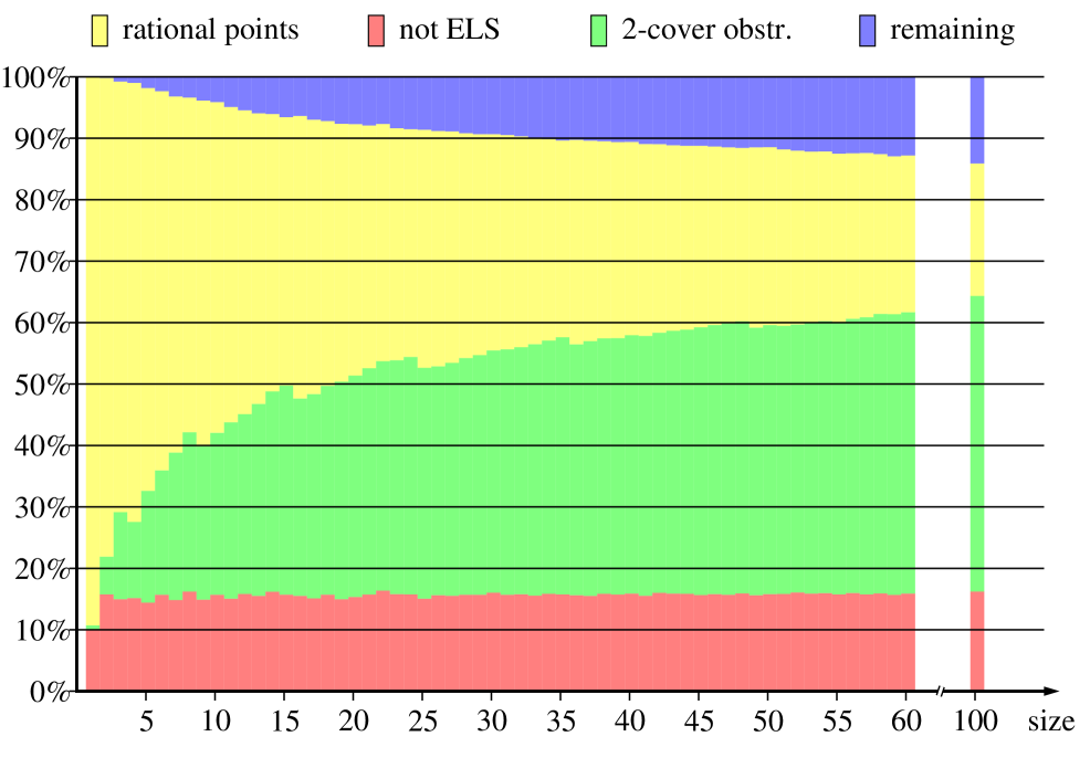
Figure 1. Proportion chart of obstructions

See Table 1 for the statistics and Figure 1 for a graph of the data. It should be noted that the samples for the various $D$ are not completely independent: Any curve sampled from $M(D)$ that happened to have all its coefficients bounded by $D^{\prime}<D$ was also included as sample from $M(D^{\prime})$.

We make a number of observations.

1. The proportion of curves with a local obstruction against rational points tends to a value near $15$% remarkably quickly.

2. As $D$ increases, the proportion of curves in $M(D)$ with a small rational point decreases in the expected way. The jumps that can be observed at $D=4,9,16,\dots$ come from additional possibilities for points at infinity or with $x=0$ that occur when the leading or trailing coefficient is a square.

3. The proportion of curves with $\mathrm{Sel}_{\mathrm{fake}}^{(2)}(C/\mathbb{Q})$ non-empty decreases more slowly. Figure 1 clearly shows that, at least for $C\in M(100)$, testing if $\mathrm{Sel}_{\mathrm{fake}}^{(2)}(C/\mathbb{Q})=\emptyset$ is a very useful criterion to decide if $C(\mathbb{Q})$ is empty, with less than 15% of undecided curves.

4. The data is inconclusive on a possible limit value for the proportion of curves $C\in M(D)$ with $\mathrm{Sel}_{\mathrm{fake}}^{(2)}(C/\mathbb{Q})=\emptyset$ as $D\to\infty$, but it suggests that it might be somewhere between 65% and 85%. It would be very interesting to find out if this limit exists and what its approximate value might be. What makes this likely to be hard is the subtle interplay between local and global information that determines the size of $\mathrm{Sel}_{\mathrm{fake}}^{(2)}(C/\mathbb{Q})$.