Suppression of absorption by quantum interference in intersubband transitions of tunnel-coupled double quantum wells

Abstract

We propose and analyze an efficient scheme for suppressing the absorption of a weak probe field based on intersubband transitions in a four-level asymmetric coupled-quantum well (CQW) driven coherently by a probe laser field and a control laser field. By using the numerical simulation, we find that the magnitude of the transient absorption of the probe field is smaller than the three-level system based on the electromagnetically induced transparency (EIT) at line center of the probe transition, moreover, comparing with the scheme in three-level asymmetric double QW system, the transparency hole of the present work is much broader. By analyzing the steady-state process analytically and numerically, our results show that the probe absorption can be completely eliminated under the condition of Raman resonance (i.e. two-photon detuning is zero). Besides, we can observe one transparency window without requiring one- or two-photon detuning exactly vanish. This investigation may provide the possible scheme for EIT in solids by using CQW.

I Introduction

The optical properties of cold atomic gases can be radically modified by laser beams1 . A strong laser light essentially influences atomic states, quantum coherence and interference between the excitation pathways controlling the optical response become possible, and the absorption of weak laser light vanishes. This effect was termed electromagnetically induced transparency (EIT)2 . The phenomenon of EIT has been deeply studied in atomic physics1 -10 , starting from its observation in sodium vapors11 , where the effect of EIT in atomic system has disclosed new possibilities for nonlinear optics and quantum information processing. For example, few works have demonstrated that EIT can be used to suppress both single-photon and two-photon absorptions in three-level atomic medium6 . The schemes for suppressing absorption of the short-wavelength light based on EIT have also been proposed9 . In particular, few authors analyzed and discussed suppressed both two- and three-photon absorptions in four-wave mixing (FWM) and hyper-Raman scattering (HRS) in resonant coherent atomic medium via EIT7 ; 8 ; 9 .

As we know, it is easy to implement EIT in optically dense atomic medium in gases phase, but it is more difficult to observe EIT in solid-state medium due to the short coherence times in solid-state system1 . Nevertheless, some investigations have demonstrated EIT effect and ultraslow optical pulse propagation in semiconductor quantum wells (QW) structure12 -16 . For example, Sadeghi et al.13 , in an asymmetric QW, have shown that EIT may be obtained with appropriate driving fields, provided that the coherence between the intersubbands considered is preserved for a sufficiently long time. So that quantum coherence and interference in QW structures have also attracted great interesting due to the potentially important applications in optoelectronics and solid-state quantum information science. In fact, except for the investigations of EIT, Autler-Townes splitting17 , gain without inversion18 , modified Rabi oscillations and controlled population transfer19 ; 20 , largely enhanced second harmonic generation21 , controlled optical bistability22 , ultrafast all-optical switching23 , phase-controlled behavior of absorption and dispersion24 , coherent population trapping25 , enhanced refraction index without absorption26 , FWM27 , and several other phenomena28 -30 , have been theoretically studied and experimentally observed in intersubband transitions of semiconductor QW. In addition, we take notice of the calculation of the model for an asymmetric semiconductor coupled double quantum well31 -34 , in which the realization of a photon switch and the optical bistability have been studied based on quantum interference between intersubband transitions in this system32 . The aim of our current study is to analyze and discuss the probe absorption properties for the two cases of transient- and steady-state processes in such system. Different from the intersubband transition in infrared region, we consider such transition in the ultraviolet or visible region, in which it has very large dipole moment length, so the optoelectonics devices may be realized with relatively smaller pulse intensity. Besides, Devices based on semiconductor QW structures have many inherent advantages, such as large electric dipole moments due to the small effective electron mass, high nonlinear optical coefficients, and a great flexibility in device design by choosing the materials and structure dimensions.

II The physical model and equations of motion

Let us consider the asymmetric semiconductor coupled double quantum well structure consisting of 10 pairs of a 51-monolayer (145Å) thick wide well and a 35-monolayer (100Å)thick narrow well, separated by a Al_0.2Ga_0.8As buffer layer33 ; 34 , as shown in Fig. 1. In this quantum well structure, the first ($n=1)$ electron level in the wide well and the narrow well can be energetically aligned with each other by applying a static electric field, while the corresponding $n=1$ hole levels are never aligned for this polarity of the field. For transitions from the wide well and the narrow well, the Coulomb interaction between electron and the hole downshifts the value of the electric field where the resonance condition is fulfilled to that corresponding to the built-in field. Level $\left|3\right\rangle$ and level $\left|4\right\rangle$, respectively corresponding the bonding state and the anti-bonding state, are tunnel-coupled new states of the first ($n=1)$ electron level in the wide well and the narrow well. The energy difference $2\Delta$ of the bonding state and anti-bonding state is determined by the level splitting in the absence of tunneling and the tunneling matrix element, and can be controlled by an electric field applied perpendicularly to coupled-quantum wells. Level $\left|1\right\rangle$ in the narrow well and level $\left|2\right\rangle$ in the wide well are localized hole states.

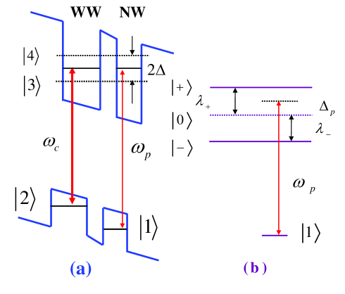
Figure 1: Conduction subband energy level diagram for an asymmetric coupled quantum wells consisting of a wide well (WW) and a narrow well (NW), as shown in Ref.33 . (a) Levels $\left|3\right\rangle$ and $\left|4\right\rangle$ are the bonding and antibonding electron state of coupled system and Levels $\left|1\right\rangle$ and $\left|2\right\rangle$ are the localized hole states. $2\Delta$, $\omega_{c}$ and $\omega_{p}$ are the energy splitting between tunnel-coupled electronic levels, frequency of the strong coupled field and the weak probe field, respectively. (b) Corresponding to the dressed-state picture for the case $\Delta_{c}=0$: subband $\left|2\right\rangle$ couple with subbands $\left|3\right\rangle$ and $\left|4\right\rangle$ simultaneously giving rise to the three dressed states $\left|+\right\rangle$, $\left|0\right\rangle$ and $\left|-\right\rangle$.

We assume the transitions $\left|2\right\rangle\leftrightarrow\left|4\right\rangle$ and $\left|2\right\rangle\leftrightarrow\left|3\right\rangle$ are simultaneously driven by a strong coupling field with the respective one-half Rabi frequencies $\Omega_{c}=\mu_{42}E_{c}/2\hbar$ and $(\Omega_{c}\mu_{32})/\mu_{42}$. At the same time, a weak probe field is applied to the transitions $\left|1\right\rangle\leftrightarrow\left|4\right\rangle$ and $\left|1\right\rangle\leftrightarrow\left|3\right\rangle$ simultaneously with the respective Rabi frequencies $\Omega_{p}=\mu_{41}E_{p}/2\hbar$ and $(\Omega_{p}\mu_{31})/\mu_{41}$. $E_{c}$ and $E_{p}$ are the amplitude of the strong-coupling field and the weak probe field, respectively. $\mu_{ij}=\mu_{ij}\cdot\widehat{e}_{L}$ is the dipole moment for the transition between levels $\left|i\right\rangle$ and $\left|j\right\rangle$ with $\widehat{e}_{L}$ being the unit polarization vector of the corresponding laser field. In schrödinger picture and in rotating-wave approximation (RWA), the semiclassical Hamiltonian describing the system under study can present as

$$H=\sum\limits_{j=1}^{4}{E_{j}\left|j\right\rangle\left\langle j\right|}-\hbar(k\Omega_{c}e^{-i\omega_{c}t}\left|3\right\rangle\left\langle 2\right|+\Omega_{c}e^{-i\omega_{c}t}\left|4\right\rangle\left\langle 2\right|+q\Omega_{p}e^{-i\omega_{p}t}\left|3\right\rangle\left\langle 1\right|+\Omega_{p}e^{-i\omega_{p}t}\left|4\right\rangle\left\langle 1\right|+H.c.).$$ (1)

Here $E_{j}=\hbar\omega_{j}$ is the energy of the subband level $\left|j\right\rangle$ ($j=1,2,3,4)$, and the parameters $k=\mu_{32}/\mu_{42}$, $q=\mu_{31}/\mu_{41}$ represent the ratios between the dipole moments of the subband transitions. Working in the interaction picture, utilizing RWA and the electric-dipole approximation (EDA), we derive the interaction Hamiltonian for the system as (assuming $\hbar=1$)

$$H_{I}=(\Delta_{c}-\Delta_{p})\left|2\right\rangle\left\langle 2\right|-(\Delta_{p}+\Delta)\left|3\right\rangle\left\langle 3\right|+(\Delta-\Delta_{p})\left|4\right\rangle\left\langle 4\right|+(\Omega_{c}\left|4\right\rangle\left\langle 2\right|+k\Omega_{c}\left|3\right\rangle\left\langle 2\right|+\Omega_{p}\left|4\right\rangle\left\langle 1\right|+q\Omega_{p}\left|3\right\rangle\left\langle 1\right|+H.c.),$$ (2)

with $H_{0}=(\omega_{p}-\omega_{c})\left|2\right\rangle\left\langle 2\right|+\omega_{p}\left|3\right\rangle\left\langle 3\right|+\omega_{p}\left|4\right\rangle\left\langle 4\right|$, $\Delta_{c}=\omega_{c}+\omega_{2}-\omega_{0}$, $\Delta_{p}=\omega_{p}-\omega_{0}$, $\omega_{0}=\frac{1}{2}(\omega_{4}+\omega_{3})$ and $\Delta=(E_{4}-E_{3})/2$. $\Delta_{p}$ is the detuning between the frequency of the probe field and the average transition frequency $\omega_{0}$, $\Delta_{c}$ is the detuning between the frequency of the strong-coupling field and the average frequency. It should be emphasized that the electron sheet density of the quantum well structure is such that electron-electron effects have very small influence in our results. Therefore, the effects of electron-electron interactions are not considered in this present work. Besides, we have regarded the $E_{1}$ as the energy origin. For simplicity, we assume that the Rabi frequency of external field $\Omega_{c}$ and $\Omega_{p}$ are real. Based on the equation of motion for density operator in the interaction picture ($\partial\rho/\partial t=-i[H_{I},\rho]+\Lambda\rho)$, we can easily derive the density matrix equations of motion as follows

$$\frac{\partial\rho_{44}}{\partial t}=i\Omega_{c}(\rho_{24}-\rho_{42})+i\Omega_{p}(\rho_{14}-\rho_{41})-(2\gamma_{41}+2\gamma_{42})\rho_{44}-\frac{\kappa}{2}(\rho_{34}+\rho_{43}),$$ (3)

$$\frac{\partial\rho_{33}}{\partial t}=ik\Omega_{c}(\rho_{23}-\rho_{32})+iq\Omega_{p}(\rho_{13}-\rho_{31})-(2\gamma_{31}+2\gamma_{32})\rho_{33}-\frac{\kappa}{2}(\rho_{34}+\rho_{43}),$$ (4)

$$\frac{\partial\rho_{22}}{\partial t}=ik\Omega_{c}(\rho_{32}-\rho_{23})+i\Omega_{p}(\rho_{42}-\rho_{24})-2\gamma_{21}\rho_{22}+2\gamma_{32}\rho_{33}+2\gamma_{42}\rho_{44},$$ (5)

$$\frac{\partial\rho_{34}}{\partial t}=i\omega_{s}\rho_{34}+ik\Omega_{c}\rho_{24}+iq\Omega_{p}\rho_{14}-i\Omega_{c}\rho_{32}-i\Omega_{p}\rho_{31}-\Gamma_{34}\rho_{34}-\frac{\kappa}{2}(\rho_{44}+\rho_{33}),$$ (6)

$$\frac{\partial\rho_{24}}{\partial t}=i(\Delta-\Delta_{c})\rho_{24}+i\Omega_{c}(\rho_{44}-\rho_{22})+ik\Omega_{c}\rho_{34}-i\Omega_{p}\rho_{21}-\Gamma_{24}\rho_{24}-\frac{\kappa}{2}\rho_{23},$$ (7)

$$\frac{\partial\rho_{14}}{\partial t}=i(\Delta-\Delta_{p})\rho_{14}+i\Omega_{p}(\rho_{44}-\rho_{11})+iq\Omega_{p}\rho_{34}-i\Omega_{c}\rho_{12}-\Gamma_{14}\rho_{14}--\frac{\kappa}{2}\rho_{13},$$ (8)

$$\frac{\partial\rho_{23}}{\partial t}=-i(\Delta+\Delta_{c})\rho_{23}-iq\Omega_{p}\rho_{21}+i\Omega_{c}\rho_{43}+ik\Omega_{c}(\rho_{33}-\rho_{22})-\Gamma_{23}\rho_{23}-\frac{\kappa}{2}\rho_{13},$$ (9)

$$\frac{\partial\rho_{13}}{\partial t}=-i(\Delta+\Delta_{p})\rho_{13}+i\Omega_{p}\rho_{43}-ik\Omega_{c}\rho_{12}+iq\Omega_{p}(\rho_{33}-\rho_{11})-\Gamma_{13}\rho_{13}-\frac{\kappa}{2}\rho_{24},$$ (10)

$$\frac{\partial\rho_{12}}{\partial t}=i(\Delta_{c}-\Delta_{p})\rho_{12}-ik\Omega_{c}\rho_{13}+iq\Omega_{p}\rho_{32}-i\Omega_{c}\rho_{14}+i\Omega_{p}\rho_{42}-\Gamma_{12}\rho_{12}-\frac{\kappa}{2}\rho_{14},$$ (11)

together with $\rho_{ij}=\rho_{ji}^{\ast}$ and the carrier conservation condition $\rho_{11}+\rho_{22}+\rho_{33}+\rho_{44}=1$. Here the population decay rates $\gamma_{il}$ (life broadening) and the dephasing decay rates $\gamma_{ij}^{dph}$ (dephasing line width corresponding to the respective transitions) are added phenomenologically in the above equations with the total decay rates (line width) being $\Gamma_{12}=\gamma_{12}^{dph}+\frac{\gamma_{2l}}{2}$, $\Gamma_{13}=\gamma_{13}^{dph}+\frac{\gamma_{3l}}{2}$, $\Gamma_{14}=\gamma_{14}^{dph}+\frac{\gamma_{4l}}{2}$, $\Gamma_{23}=\gamma_{23}^{dph}+\frac{\gamma_{2l}+\gamma_{3l}}{2}$, $\Gamma_{24}=\gamma_{24}^{dph}+\frac{\gamma_{2l}+\gamma_{4l}}{2}$, and $\Gamma_{34}=\gamma_{34}^{dph}+\frac{\gamma_{3l}+\gamma_{4l}}{2}$, where $\gamma_{il}$ is determined by longitudinal optical (LO) phonon emission events at low temperature, the $\gamma_{ij}^{dph}$ is determined by electron-electron, interface roughness, and phonon scattering processes16 . The population decay rates can be calculated, and as we know, the initially nonthermal carrier distribution is quickly broadened due to inelastic carrier-carrier scattering, with the broadening rate increasing as carrier density is increased. For the temperatures up to 10 K, the carrier density smaller than $10^{11}$ cm^-2, the dephasing decay rates $\gamma^{dph}_{ij}$ can be estimated according to Ref.23 . Besides, the dephasing-type broadening $\kappa=\sqrt{\gamma_{3l}\gamma_{4l}}$ denotes the cross coupling of states $\left|4\right\rangle$ and $\left|3\right\rangle$ via the LO phonon decay. A more complete theoretical treatment taking into account these process for the dephasing rates is though interesting but beyond the scope of this paper.

In the following analysis, we choose the parameters are set to be $\mu_{32}=\mu_{42}=\mu_{c}$ and $\mu_{31}=\mu_{41}=\mu_{p}$ (i.e. $k=1$ and $q=1$); and we take $\Gamma_{12}=0$ for the lifetime of levels $\left|2\right\rangle$ and $\left|1\right\rangle$ according to the Ref.35 . By a straightforward semiclassical analysis, the above matrix elements can be used to calculate the total linear complex susceptibility $\chi$ of the probe transitions $\left|1\right\rangle\rightarrow\left|3\right\rangle$ and $\left|1\right\rangle\rightarrow\left|4\right\rangle$, i.e.

$$\chi=\frac{N\left|{\mu_{p}}\right|^{2}(\rho_{13}+\rho_{14})}{2\hbar\varepsilon_{0}\Omega_{p}},$$ (12)

where $N$ is the electron number density in the medium and $\varepsilon_{0}$ is the permittivity of free space. Based on the Eq. (12), one can find that the gain-absorption coefficient for the probe field coupled to the transitions $\left|1\right\rangle\leftrightarrow\left|3\right\rangle$ ($\left|4\right\rangle)$ is proportional to the term Im$(\rho_{13}+\rho_{14})$ in the limit of a weak probe field. Im$(\rho_{13}+\rho_{14})>0$ presents the absorption of the probe field, Im$(\rho_{13}+\rho_{14})<0$ presents the amplified of the probe field. In the following, we investigate the absorption properties of such a weak probe field for the transient- and steady-state processes. We begin by solving numerically the time-dependent differential equations (3)-(11) by using Runge-Kutta algorithm with the initial conditions $\rho_{11}(0)=1$, $\rho_{22}(0)=\rho_{33}(0)=\rho_{44}(0)=0$ and $\rho_{ij}(0)=0$ for $i\neq j$ ($i,j=1,2,3,4)$. Note that, the parameters $\Omega_{c}$, $\Omega_{p}$, $\Delta_{c}$, $\Delta_{p}$, $\Delta$, $\gamma_{ij}$, $\gamma_{ij}^{dph}$ are defined as units of $\gamma$ in this present paper.

III The probe absorption under the transient-state process

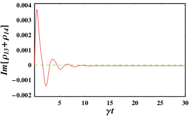
Figure 2: Transient absorption and amplification response for a probe laser field with parameters being $\Omega_{p}=0.01\gamma$, $\Delta=\gamma$, $\Delta_{c}=\Delta_{p}=0$, $\gamma_{3l}=\gamma_{4l}=0.4\gamma$, $\gamma_{14}^{dph}=\gamma_{24}^{dph}=\gamma_{13}^{dph}=\gamma_{23}^{dph}=0.1\gamma$.

Firstly, we examined the probe absorption under the transient-state process by using different sets of parameters.

We show in Fig.2 the time evolution of the absorption coefficient Im$(\rho_{13}+\rho_{14})$ under the Raman resonant condition $\Delta_{c}=\Delta_{p}$ with the parameters-value $\Omega_{p}=0.01\gamma$, $\Omega_{c}=4\gamma$, $\Delta=\gamma$, $\gamma_{3l}=\gamma_{4l}=0.4\gamma$ and $\gamma_{14}^{dph}=\gamma_{24}^{dph}=\gamma_{13}^{dph}=\gamma_{23}^{dph}=0.1\gamma$. The probe field shows the oscillatory behavior versus the time before reaching the steady state, which just like in high density atomic system. The probe absorption increases rapidly to a maximum peak value, then it decreases gradually to a peak value and again increases with increase of the evolution time, up to a negative large steady-state value below the zero-absorption line. Comparing with the three-level EIT system, the transient behavior of the probe field can be tuned by adjusting the coherent tuneling (coupling) between the two upper levels $\left|3\right\rangle$ and $\left|4\right\rangle$ across a thin barrier, we can expect that the coupling strength, i.e., the energy splitting $2\Delta$, must play an important role in controlling the transient behavior of the probe field in such an asymmetric double QW system.

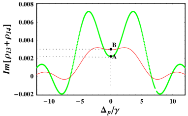
Figure 3: The probe absorption as a function of dimensionless probe detuning $\Delta_{p}/\gamma$ for the transition under the condition of transient-state process. Solid red curve: $\Delta=0$; dot green curve: $\Delta=\gamma$. Other fitting parameters used are $\Omega_{c}=2\gamma$, $\Omega_{p}=0.01\gamma$, $\Delta_{c}=0$, $\gamma_{3l}=\gamma_{4l}=0.4\gamma$, $\gamma_{14}^{dph}=\gamma_{24}^{dph}=\gamma_{13}^{dph}=\gamma_{23}^{dph}=0.1\gamma$.

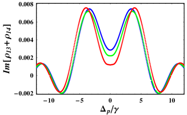
Figure 4: Imaginary part of the susceptibility of the probe transition as a function of dimensionless detuning $\Delta_{p}/\gamma$ under the condition of transient-state process with $\Omega_{c}=1.5\gamma$ (blue line), $\Omega_{c}=2\gamma$ (green line) and $\Omega_{c}=1\gamma$ (red line). Other parameters are $\Omega_{p}=0.01\gamma$, $\Delta=\gamma$, $\Delta_{c}=0$, $\gamma_{3l}=\gamma_{4l}=0.4\gamma$, $\gamma_{14}^{dph}=\gamma_{24}^{dph}=\gamma_{13}^{dph}=\gamma_{23}^{dph}=0.1\gamma$.

We show in Fig.3 the magnitudes of the transient absorption of the probe field versus the probe detuning $\Delta_{p}/\gamma$. At the line center of the probe transition $\Delta_{p}=0$, the magnitude of the transient absorption of the probe field at point A corresponding to the splitting $2\Delta$ is much smaller than the magnitude of the probe field at point B for the three-level EIT corresponding to $\Delta=0$. With appropriate values of parameters we obtain the absorption spectra shown in Fig.4 for different intensities of the strong-coupling field. With the increasing the intensity of the strong-coupling field, the absorption deep of the probe field moves small accordingly, as expected for coherent EIT. At the same time, with a larger intensity of the control field the transparency width increases, which corresponds to the splitting between the two upper levels $\left|3\right\rangle$ and $\left|4\right\rangle$. From the above analysis, we can conclude that the probe absorption at the line center ($\Delta_{p}=0)$ can be considerably suppressed due to the fact of the splitting $2\Delta$.

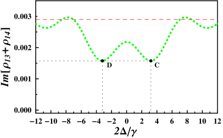
Figure 5: The probe absorption as a function of dimensionless splitting $\Delta/\gamma$ between $\left|3\right\rangle$ and $\left|4\right\rangle$ under the condition of transient-state process (green curve). The dashed red line stands for the magnitude of the probe absorption for the three-level EIT at $\Delta_{p}=\Delta_{c}=0$. Other fitting parameters used are $\Delta_{p}=0$, $\Delta_{c}=0$,$\Omega_{p}=0.01\gamma$, $\Omega_{c}=2\gamma$ $\gamma_{3l}=\gamma_{4l}=0.4\gamma$, $\gamma_{14}^{dph}=\gamma_{24}^{dph}=\gamma_{13}^{dph}=\gamma_{23}^{dph}=0.1\gamma$.

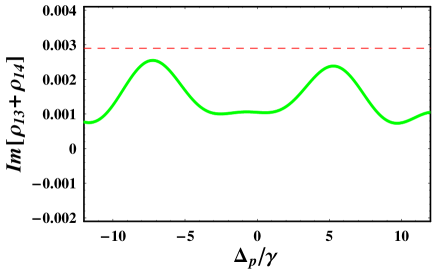
Figure 6: The probe transition as a function of dimensionless detuning $\Delta_{p}/\gamma$ under the condition of transient-state process for the Ramman resonance $\Delta_{c}=\Delta_{p}$ (green curve). The dashed line stands for the magnitude of the probe absorption for three-level EIT at $\Delta_{c}=\Delta_{p}=0$. Other fitting parameters being $\Omega_{p}=0.01\gamma$, $\Omega_{c}=2\gamma$, $\Delta=\gamma$, $\gamma_{3l}=\gamma_{4l}=0.4\gamma$, $\gamma_{14}^{dph}=\gamma_{24}^{dph}=\gamma_{13}^{dph}=\gamma_{23}^{dph}=0.1\gamma$.

The calculated probe absorption coefficient of such a weak probe laser versus the splitting ($2\Delta$) between $\left|3\right\rangle$ and $\left|4\right\rangle$ for the probe and coupling laser detunings $\Delta_{p}=\Delta_{c}=0$ is shown in Fig.5, in which the dashed red line stands for the magnitude of the probe absorption for the standard three-level EIT and the positions C and D correspond to the minimum of the probe absorption. We observe that the magnitude of the transient absorption of the probe field with the inclusion of the splitting $2\Delta$ is almost lower than the magnitude of the probe absorption with the three level EIT at $\Delta_{p}=\Delta_{c}=0$. As shown in Fig.6, we plot absorption profiles versus the probe detuning $\Delta_{p}$ in the case of two-photon Raman resonance $\Delta_{p}=\Delta_{c}$. For this case, we find that the maximal absorption peak is always located below the the probe absorption of the standard three-level EIT.

IV The probe absorption under steady-state condition

Then we examined the probe absorption under the steady-state condition, i.e., $\partial\rho_{ij}/\partial t=0$. The general steady-state solutions for Eqs. (3)-(11) can be derived analytically (analyzing with two resonant coupling and probe fields), but the tedious and intricate expressions for the solutions corresponding to the situation of an off-resonant coupling field offers no clear physical sight. So we performance the numerical calculation here. The present process is most clearly understood according to the dressed states produced by the strong coupling field $\omega_{c}$ as shown in Fig. 1(b), i.e., the transitions $\left|2\right\rangle\leftrightarrow\left|3\right\rangle$ and $\left|2\right\rangle\leftrightarrow\left|4\right\rangle$ together with the coupling field are treated as a total system forming the dressed states. Under the action of the strong coherent coupling field, levels $\left|3\right\rangle$ and $\left|4\right\rangle$ should be split into three dressed-state levels $\left|\pm\right\rangle$ and $\left|0\right\rangle$. The energy eigenstates of the dressed states for the $\Delta_{c}=0$ case are written as follows

$$\left|+\right\rangle=-\frac{\Omega_{c}}{\sqrt{\Delta^{2}+2\Omega_{c}^{2}}}\left|2\right\rangle-\frac{1}{2}\frac{\Delta-\sqrt{\Delta^{2}+2\Omega_{c}^{2}}}{\sqrt{\Delta^{2}+2\Omega_{c}^{2}}}\left|3\right\rangle+\frac{1}{2}\frac{\Delta+\sqrt{\Delta^{2}+2\Omega_{c}^{2}}}{\sqrt{\Delta^{2}+2\Omega_{c}^{2}}}\left|4\right\rangle,$$ (13)

$$\left|0\right\rangle=\frac{\Delta}{\sqrt{\Delta^{2}+2\Omega_{c}^{2}}}\left|2\right\rangle-\frac{\Omega_{c}}{\sqrt{\Delta^{2}+2\Omega_{c}^{2}}}\left|3\right\rangle+\frac{\Omega_{c}}{\sqrt{\Delta^{2}+2\Omega_{c}^{2}}}\left|4\right\rangle,$$ (14)

$$\left|-\right\rangle=\frac{\Omega_{c}}{\sqrt{\Delta^{2}+2\Omega_{c}^{2}}}\left|2\right\rangle+\frac{1}{2}\frac{\Delta+\sqrt{\Delta^{2}+2\Omega_{c}^{2}}}{\sqrt{\Delta^{2}+2\Omega_{c}^{2}}}\left|3\right\rangle-\frac{1}{2}\frac{\Delta-\sqrt{\Delta^{2}+2\Omega_{c}^{2}}}{\sqrt{\Delta^{2}+2\Omega_{c}^{2}}}\left|4\right\rangle.$$ (15)

The corresponding energy eigenvalues are given by $\lambda_{0}=0$ and $\lambda_{\pm}=\pm\sqrt{\Delta^{2}+2\Omega_{c}^{2}}$. And the dressed-state transition dipole moments can be derived as: $\mu_{+1}=\left\langle+\right|P\left|1\right\rangle=\mu_{p}$, $\mu_{01}=\left\langle 0\right|P\left|1\right\rangle=0$, $\mu_{-1}=\left\langle-\right|P\left|1\right\rangle=\mu_{p}$, where $P=\mu_{p}(\left|3\right\rangle\left\langle 1\right|+\left|4\right\rangle\left\langle 1\right|)$ represents the polarization operator of the probe transition.

Based on the above analysis, it is straightforwardly shown that the transition between dressed-levels $\left|0\right\rangle$ and $\left|1\right\rangle$ is forbidden due to the couplings of $\left|1\right\rangle\leftrightarrow\left|3\right\rangle$ and $\left|1\right\rangle\leftrightarrow\left|4\right\rangle$. As shown in Fig.7, we can observe two symmetric absorption peaks with same amplitude on the probe spectra in the case of $\Delta_{c}=0$ because of the relation $\mu_{+1}=\mu_{-1}$. The two absorption peaks correspond respectively to the dressed-state transitions $\left|1\right\rangle\leftrightarrow\left|+\right\rangle$ and $\left|1\right\rangle\leftrightarrow\left|-\right\rangle$, so the peaks are always located at $\Delta_{p}=\pm\sqrt{\Delta^{2}+2\Omega_{c}^{2}}$, and the difference between them becomes larger with increasing $\Omega_{c}$. Since the transition $\left|1\right\rangle\leftrightarrow\left|0\right\rangle$ in the dressed-state picture is interference-cancelled out and this interference always makes a negative contribution to the probe absorption, thus it is easy to understand that the probe absorption at the line center can be approximately equal to zero, i.e., the probe absorption can be completely suppressed, so that the absorption peak at the line center is too small to be observed. As shown in Fig.8, we plot the probe absorption profile versus the probe detuning $\Delta_{p}$. One can find that the probe absorption spectra are always approximately equal to zero within the range of the splitting $2\Delta$ between two tunnel-coupled levels ($\left|3\right\rangle$ and $\left|4\right\rangle)$. This means that if the two-photon Raman resonance is satisfied ($\Delta_{p}=\Delta_{c}$), we can observe the transparency window without requiring one- or two-photon detunings exactly vanish.

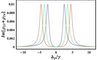
Figure 7: Imaginary part of the susceptibility of the probe transition as a function of dimensionless detuning $\Delta_{p}/\gamma$ under the condition of steady-state process with $\Omega_{c}=2\gamma$ (blue curve), $\Omega_{c}=3\gamma$ (green curve) and $\Omega_{c}=4\gamma$ (red curve). Other parameters used are $\Omega_{p}=0.01\gamma$, $\Delta=\gamma$, $\Delta_{c}=0$, $\gamma_{3l}=\gamma_{4l}=0.4\gamma$, $\gamma_{14}^{dph}=\gamma_{24}^{dph}=\gamma_{13}^{dph}=\gamma_{23}^{dph}=0.1\gamma$.

Figure 8: Imaginary part of the susceptibility of the probe transition as a function of dimensionless detuning $\Delta_{p}/\gamma$ under the condition of steady-state process for the Raman resonance ($\Delta_{c}=\Delta_{p}$) with the parameters being $\Omega_{p}=0.01\gamma$, $\Omega_{c}=4\gamma$, $\Delta=\gamma$, $\gamma_{3l}=\gamma_{4l}=0.4\gamma$, $\gamma_{14}^{dph}=\gamma_{24}^{dph}=\gamma_{13}^{dph}=\gamma_{23}^{dph}=0.1\gamma$.

V Discussions and Conclusion

We now give a brief discussion on the practical setup. The asymmetric semiconductor coupled double QW structure, considered here, consists of 10 pairs of a 51-monolayer (145Å) thick wide well and a 35-monolayer (100Å)thick narrow well, separated by a Al_0.2Ga_0.8 As buffer layer, as shown in Fig. 1. The probe field propagates in the polarization direction. As in the report in Ref.33 , we consider a transverse magnetic polarized probe incident at an angle of 45 degrees with respect to the growth axis so that all transition dipole moments include a factor $1/\sqrt{2}$ as subband transitions are polarized along the growth axis. In the sections III and IV, all the calculations have assumed that the parameters $\Omega_{c}$, $\Omega_{p}$, $\Delta_{c}$, $\Delta_{p}$, $\Delta$, $\gamma_{ij}$, $\gamma_{ij}^{dph}$ are defined as units of $\gamma$ in this present paper. By setting $\gamma=1.25$THz, the corresponding parameters value in the present paper are respectively as $\gamma_{3l}=\gamma_{4l}=0.5$THz, $\gamma_{14}^{dph}=\gamma_{24}^{dph}=\gamma_{13}^{dph}=\gamma_{23}^{dph}=0.125$THz, $\Omega_{p}=0.0125$THz, The maximal value of $\Omega_{c}$ is about 5THz, which can be realized with current experimental technology 33 .

In conclusion, in the present paper, we have analyzed and discussed the probe absorption properties in a tunnel-coupled double quantum wells under the conditions for the transient regime and the steady-state process by using the detailed numerical simulations based on the density matrix equations (3)-(11). Besides, we analytically analyze probe absorption mechanism for the steady-state process in the dressed-state picture. In the steady-state process, we show that the probe absorption can be largely suppressed with the coupling field resonance ($\Delta_{c}=0$), and be eliminated completely under the condition of Raman resonance ($\Delta_{p}=\Delta_{c}$) within the range of the $2\Delta$. In the transient-state process, we show that the magnitude of the probe absorption at the line center of the probe transition $\Delta_{p}=0$ can be greatly suppressed. Comparing with the EIT scheme in the three-Level QW structures12 -14 , our results show that the transparency hole is much broader due to the fact that the existence of the tunnel-coupling splitting $2\Delta$. Besides, we do not require that the one- or two-photon detunings is exactly zero. As a result, the present investigation confirm the possibility of obtaining EIT in solids by using asymmetric tunnel-coupled QW. Our calculations also provide a guideline for the optimal design to achieve very fast and low-threshold all-optical switches in such semiconductor systems which is much more practical than that in atomic system because of its flexible design and the controllable coherent coupling strength.

The research is supported in part by National Fundamental Research Program of China 2005CB724508, by National Natural Science Foundation of China under Grant Nos. 10704017, 10634060, 90503010 and 10575040.

References

- (1) Harris S E, 1997 Phys. Today 50 36; Fleishhauer M, Imamoglu A, and Marangos J P, 2005 Rev. Mod. Phys. 77 633 ; Lukin M D, 2003 Rev. Mod. Phys. 75 457; Lukin M D, Hemmer P, and Scully M O, Adv. At., Mol., 2000 Opt. Phys. 42 347.
- (2) Harris S E, Field J E, and Imamoglu A, 1990 Phys. Rev. Lett. 64 1107.
- (3) Arimondo E, in Progress in Optics, edited by E. Wolf (Elsevier, Amsterdam, 1996), p257.
- (4) Hau L V et al., 1999 Nature 397 594; Liu C et al., 2001 Nature 409 490.
- (5) Agarwal G S and Harshawardhan W, 1996 Phys. Rev. Lett. 77 1039 ; Li Y and Xiao M, 1996 Opt. Lett. 21 1064.
- (6) Yan M, Rickey E, and Zhu Y, 2001 Phys. Rev. A 64 043807; Yan M, Rickey E, and Zhu Y, 2001 Opt. Lett. 26 548.
- (7) Wu Y and Yang X, 2004 Phys. Rev. A 70 053818; Wu Y, 2005 Phys. Rev. A 71 053820; Wu Y and Deng L, 2004 Phys. Rev. Lett. 93 143904; Wu Y and Yang X, 2005 Phys. Rev. A 71 053806.
- (8) Wu J H et al., 2003 Opt. Lett. 28 654.
- (9) Harris S E and Yamamoto Y, 1998 Phys. Rev. Lett. 81 3611.
- (10) Wu Y, Saldana J and Zhu Y, 2003 Phys. Rev. A 67 013811; ibid, 2003 Opt. Lett. 28 631.
- (11) Alzetta G, Gozzini A, Moi L, Orriols G, 1976 Nuovo Cim. B 36 5; Arimondo E, Orriols G, 1976 Lett. Nuovo Cim. D 17 333.
- (12) Nikonov D E, Imamoglu A, Scully M O, 1999 Phys. Rev. B 59 12212.
- (13) Sadeghi S M, Leffler S R, Meyer J, 1999 Phys. Rev. B 59 15388; Sadeghi S M, Meyer J, 2000 Phys. Rev. B 61 16841; Sadeghi S M, van Driel H M, 2001 Phys. Rev. B 63 045316.
- (14) Silvestri L, Bassanil F, Czajkowski G, Davoudi B, 2002 Eur. Phys. J. B 27 89.
- (15) Phillips M and Wang H, 2003 Opt. Lett. 28 831; Ginzburg P and Orenstein M, 2006 Opt. Express. 14 12467.
- (16) Serapiglia G B, Paspalakis E, Sirtori C, Vodopyanov K L, and Phillips C C, 2000 Phys. Rev. Lett. 84 1019.
- (17) Dynes J F, Frogley M D, Beck M, Faist J, and Phillips C C, 2005 Phys. Rev. Lett. 94 157403.
- (18) Imamoglu A and Ram R J, 1994 Opt. Lett. 19 1744; Lee C R, et al., 2005 Appl. Phys. Lett. 86 201112.
- (19) Bastista A A and Citrin D S, 2004 Phys. Rev. Lett. 92 127404; ibid, 2006 Phys. Rev. B, 74 195318.
- (20) Paspalakis E, Tsaousidou M and Terzis A F, 2006 Phys. Rev. B, 73 125344.
- (21) Tsang L, Ahn D, and Chuang S L, 1988 Appl. Phys. Lett. 52 697; Rosencher E and Bois P, 1991 Phys. Rev. B 44 11315; Schmidt H and Imamoglu A, 1996 Opt. Commun. 131 333.
- (22) Joshi A and Xiao M, 2004 Appl. Phys. B 79 65; Wijewardane H O and Ullrich C A, 2004 Appl. Phys. Lett. 84 3984.
- (23) Schmidt H et al., 1997 Appl. Phys. Lett. 70 3455; Wu J H, Gao J Y, Xu J H, Silvestri L, Artoni M, La Rocca G C, Bassani F, 2005 Phys. Rev. Lett. 95 057401.
- (24) Dynes J F and Paspalakis E, 2006 Phys. Rev. B 73 233305.
- (25) Dynes J F, Frogley M D, Rodger J and Phillips C C, Phys. Rev. B 72 085323.
- (26) Sadeghi S M, van Driel H M and Fraser J M, 2000 Phys. Rev. B 62 15386.
- (27) Paspalakis E, Kanaki A and Terzis A F, 2007 Proc. Of SPIE 6582 65821N.
- (28) Sun H, Gong S Q, Niu Y P, Jin S Q, Li R X, and Xu Z Z, 2006 Phys. Rev. B 74 155314.
- (29) Heyman J N, et al., 1994 Phys. Rev. Lett. 72 2183; Craig K, et al., 1996 Phys. Rev. Lett. 76 2382; Galdrikian B and Birnir B, 1996 Phys. Rev. Lett. 76 3308; Nikonov D E, et al., 1997 Phys. Rev. Lett. 79 4633.
- (30) Li J Z and Ning C Z, 2003 Phys. Rev. Lett. 91 097401; Olaya-Castro A, et al., 2003 Phys. Rev. B 68 155305; Luo C W, et al., 2004 Phys. Rev. Lett. 92 047402; Muller T, et al., 2004 Phys. Rev. B 70 155324.
- (31) Vasko F T and Raichev O E, 1995 Phys. Rev. B 51 16965.
- (32) Xue Y, et al., 2005 Opt. Commun. 249 231; Li J H, 2007 Opt. Commun. 274 366.
- (33) Roskos H G, et al., 1992 Phys. Rev. Lett. 68 2216.
- (34) Luo M S C, et al., 1993 Phys. Rev. B 48 11043; Planken P C M, et al., 1993 Phys. Rev. B 48 4903.
- (35) Neogi. A, Yoshida. H, Mozume. T, Wada. O, 1999 Opt. Commun. 159 225