Effects of atomic coherence on propagation, absorption, and amplification of light Optical solitons; nonlinear guided waves Quantum wells

Slow optical solitons via intersubband transitions in a semiconductor quantum well

Abstract

We show the formation of bright and dark slow optical solitons based on intersubband transitions in a semiconductor quantum well (SQW). Using the coupled Schrödinger-Maxwell approach, we provide both analytical and numerical results. Such a nonlinear optical process may be used for the control technology of optical delay lines and optical buffers in the SQW solid-state system. With appropriate parameters, we also show the generation of a large cross-phase modulation (XPM). Since the the intersubband energy level can be easily tuned by an external bias voltage, the present investigation may open the possibility for electrically controlled phase modulator in the solid-state system.

Solitons describe a class of fascinating shaping-preserving wave propagation phenomena in nonlinear media. Over the past few years, the subject of extensive theoretical and experimental investigations on solitons in optical fibers[1, 2], cold-atom media[3, 4, 5, 6, 7], Bose-Einstein condensates (BEC)[8, 9], and other nonlinear media[10], has received a great deal of attentions mainly due to that these special types of wave packets are formed as the result of interplay between nonlinearity and dispersion properties of medium under excitations, and can lead to undistorted propagation over extended distance. In the optical domain, most optical solitons are produced with intense electromagnetic fields, and far-off resonance excitation schemes are generally employed in order to avoid unmanageable optical field attenuation and distortion [1]. As a result, optical solitons produced in this way generally travel with a propagation speed very close to the speed of light in vacuum. As well known, the wave propagation velocity in highly resonant medium can be significant reduced via electromagnetically induced transparency (EIT) technique [11] or Raman-assisted interference effects. Recently, ultraslow optical solitons including two-color solitons with very low group velocities based on EIT technique or Raman-assisted interference effects, have been studied in atomic medium [3, 4, 5, 6, 7].

There is a great interest in extending these studies to semiconductors, not only for the understanding of the nature of quantum coherence in semiconductors but also for the possible implementation of optical devices such as XPM phase shifter [12], switches [13], etc. It is well known, in the conduction band of semiconductor quantum structure, that the confined electron gas exhibits atomic-like properties. For example, it has been shown that they can lead to gain without inversion [14, 15, 16], coherently controlled photocurrent generation [17], electron intersubband transmissions [18], and EIT [19, 20], slow light [21], interferences [22], optical bistability , etc. Devices based on intersubband transitions in SQW structures have many inherent advantages such as large electric dipole moments due to the small effective electron mass, high nonlinear optical coefficients, and a great flexibility in device design by choosing the materials and structure dimensions. Furthermore, the transition dipole energies can be controlled by an external bias voltage. The implementation of XPM phase shift in semiconductor-based devices is very attractive from a viewpoint of applications, such as electro-optical modulators.

In this paper, we show the formation of ultra-slow bright and dark solitons in semiconductor double quantum wells using intersubband transitions by applications of a pulsed probe field and a continuous wave (cw) strong control laser field. By choosing appropriate parameters, we also show the generation of a large XPM phase shift. As shown in Fig. 1, we consider a quantum well structure with three energy levels that forms the well known cascade configuration [24]. $\omega_{21}$ and $\omega_{32}$ present the energy differences of the $\left|1\right\rangle\leftrightarrow\left|2\right\rangle$ and $\left|2\right\rangle\leftrightarrow\left|3\right\rangle$, respectively. As a rule, such SQW samples are grown by molecular beam epitaxy (MBE) method. The sample consists 30 periods, each with 4.8 nm $\mbox{In}_{0.47}\mbox{Ga}_{0.53}\mbox{As}$, 0.2 nm $\mbox{Al}_{0.48}\mbox{In}_{0.52}\mbox{As}$, and 4.8nm $\mbox{In}_{0.47}\mbox{Ga}_{0.53}\mbox{As}$ coupled quantum wells, separated by modulation-doped 36 nm $\mbox{Al}_{0.48}\mbox{In}_{0.52}\mbox{As}$ barriers. The sample can be designed to have desired transition energies, i.e., $E_{12}$ in the range of 185 meV and $E_{23}$ in the range of 124 meV. Here, we consider a transverse magnetic polarized probe incident at an angle of 45 degrees with respect to the growth axis so that all transition dipole moments include a factor $1/\sqrt{2}$ as intersubband transitions are polarized along the growth axis. The sheet electron density is about $4.7\times 10^{11}\mbox{cm}^{-2}$. By using the standard approach (this method has described quantitatively the results of several literature [13, 15, 16, 18, 20, 25, 26]), under the rotating-wave and electro-dipole approximations the semiclassical Hamiltonian describing the electron-field interaction for the system under study in the Schrödinger picture, is given by

$$H=\sum\limits_{j=1}^{3}{E_{j}\left|j\right\rangle\left\langle j\right|}-\hbar(\Omega_{c}e^{-i\theta_{c}}\left|3\right\rangle\left\langle 2\right|+\Omega_{p}e^{-i\theta_{p}}\left|2\right\rangle\left\langle 1\right|+h.c.),$$ (1)

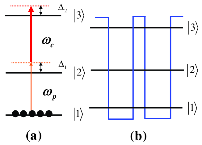
Figure 1: (a)Schematic energy level arrangement for the quantum wells under consideration here. Subband levels are labeled as $\left|1\right\rangle$, $\left|2\right\rangle$, and $\left|3\right\rangle$, respectively. The subband transition $\left|1\right\rangle\leftrightarrow\left|2\right\rangle$ is driven by an weak probe field with central frequency $\omega_{p}$ and the subband transition $\left|2\right\rangle\leftrightarrow\left|3\right\rangle$ is coupled by a control field with central frequency $\omega_{c}$. (b) Schematic three-level cascade electronic system synthesized in a semiconductor quantum well.

where the symbol h.c. means the Hermitian conjugate, $\theta_{n}=k_{n}\cdot r-\omega_{n}t$ corresponds to the positive frequency part of the respective optical field, $\Omega_{n}(n=p,c)$ are one-half Rabi frequencies for the relevant laser-driven intersubband transitions, and $E_{j}=\hbar\omega_{j}(j=1-3)$ is the energy of the subband $\left|j\right\rangle$. For simplicity, in following analysis we will take $\omega_{1}=0$ for the ground-state level $\left|1\right\rangle$ as the energy origin. Turning to the interaction picture, with the assumption of $\hbar=1$, the free and the interaction Hamiltonian can be respectively rewritten as follows

$$H_{0}=\omega_{p}\left|2\right\rangle\left\langle 2\right|+(\omega_{p}+\omega_{c})\left|3\right\rangle\left\langle 3\right|,$$ (2)

$$H_{I}=-\Delta_{1}\left|2\right\rangle\left\langle 2\right|-\Delta_{2}\left|3\right\rangle\left\langle 3\right|-(\Omega_{c}e^{ik_{c}\cdot r}\left|3\right\rangle\left\langle 2\right|+\Omega_{p}e^{ik_{p}\cdot r}\left|2\right\rangle\left\langle 1\right|+h.c.),$$ (3)

where the intersubband transition detunings of the two optical fields are defined respectively by $\Delta_{1}=\omega_{p}-E_{2}$ and $\Delta_{2}=\omega_{p}+\omega_{c}-E_{3}$. Let us assume the electronic wave function of the form

$$\left|\psi\right\rangle=A_{1}\left|1\right\rangle+A_{2}e^{ik_{p}\cdot r}\left|2\right\rangle+A_{3}e^{i(k_{p}+k_{c})\cdot r}\left|3\right\rangle,$$ (4)

together with $A_{j}(j=1,2,3)$ being the time-dependent probability amplitudes of finding the electron in subbands $\left|j\right\rangle$. By using the Schrödinger equation in the interaction picture $i\partial\left|\psi\right\rangle/\partial t=H_{I}\left|\psi\right\rangle$ for the three level model, the equations of the motion for the probability amplitude of the electronic wave functions and the wave equation for the time-dependent probe field can be readily obtained as

$$\frac{\partial A_{2}}{\partial t}=i(\Delta_{1}+i\gamma_{2})A_{2}+i\Omega_{c}^{*}A_{3}+i\Omega_{p}A_{1},$$ (5)

$$\frac{\partial A_{3}}{\partial t}=i(\Delta_{2}+i\gamma_{3})A_{3}+i\Omega_{c}A_{2},$$ (6)

$$\left|{A_{1}}\right|^{2}+\left|{A_{2}}\right|^{2}+\left|{A_{3}}\right|^{2}=1,$$ (7)

$$\frac{\partial\Omega_{p}}{\partial z}+\frac{1}{c}\frac{\partial\Omega_{p}}{\partial t}=i\frac{2N\omega_{p}\left|{\mu_{21}}\right|^{2}}{c}A_{2}A_{1}^{*},$$ (8)

with $N$ and $\mu_{12}$ being the concentration and the dipole moment between states $\left|1\right\rangle$ and $\left|2\right\rangle$, respectively. In writing Eq. (8), we have assumed collinear propagation geometry and applied slowly varying envelope approximation. $\gamma_{2}$ and $\gamma_{3}$ denote the total decay rates of the subbands $\left|2\right\rangle$ and $\left|3\right\rangle$, which are added phenomenologically [13, 18] in the above coupled amplitude equations. In semiconductor quantum wells, the overall decay rate $\gamma_{i}$ of the subband $\left|i\right\rangle$ comprises a population-decay contribution $\gamma_{il}$ as well as a dephasing contribution $\gamma_{id}$, i.e., $\gamma_{i}=\gamma_{il}+\gamma_{id}$. the former $\gamma_{il}$ is due to longitudinal optical (LO) photon emission events at low temperature. The latter $\gamma_{id}$ may originate not only from electron-electron scattering and electron-phonon scattering, but also from inhomogeneous broadening due to the scattering on interface roughness. The population decay rates can be calculated by solving the effective mass Schrödinger equation. For the temperatures up to 10 K, the carrier density smaller than $10^{12}$ $\mbox{cm}^{-2}$, the dephasing decay rates $\gamma^{dph}_{ij}$ can be estimated according to Ref.[13]. For the SQW structure considered here, the total decay rates turn out to be $\gamma_{2}=\gamma_{3}=5\mbox{meV}$. A more complete theoretical treatment taking into account these processes for the dephasing rates is though interesting but beyonds the scope of this paper.

In order to describe clearly the interplay between the dispersion and nonlinear effects of the SQW system interacting with two optical fields (probe and control fields), we now first focus on the dispersion properties of the system. It requires perturbation of the system respective to the first order of probe field $\Omega_{p}$ while keeping full orders of control field $\Omega_{c}$. In the following, we show effects from higher-order $\Omega_{p}$, and those required to balance the dispersion effect, resulting the formation of ultraslow solitons. From Eqs. (5-8), it is readily obtain that [27, 28]

$$\frac{\partial\Omega_{p}}{\partial z}+\frac{1}{c}\frac{\partial\Omega_{p}}{\partial t}=iA_{1}^{*}[K(\hat{\omega})-\frac{\hat{\omega}}{c}](\Omega_{p}A_{0}),$$ (9)

where $i\partial/\partial t$ is a differential operator and with sufficiently intense control field we have

$$K(\hat{\omega})=\frac{\hat{\omega}}{c}+\frac{\epsilon_{12}(\hat{\omega}+\Delta_{2}+i\gamma_{3})}{\left|{\Omega_{c}}\right|^{2}-(\hat{\omega}+\Delta_{1}+i\gamma_{2})(\hat{\omega}+\Delta_{2}+i\gamma_{3})}\simeq K_{0}+\frac{\hat{\omega}}{v_{g}}+K_{2}\hat{\omega}^{2}+O(\hat{\omega}^{3}),$$ (10)

where $\epsilon_{12}=2N\omega_{p}\left|{\mu_{12}}\right|^{2}/c$ and higher-order derivative terms have been neglected. The physical interpretation of Eq. (10) is rather clear. $K_{0}=\Phi+i\alpha$ describes the phase shift $\Phi$ per unit length and the absorption coefficient $\alpha$ of the pulsed probe field, $K_{1}$ gives the group velocity $V_{g}=\mbox{Re}[1/K_{1}]$, and $K_{2}$ represents the group-velocity dispersion that contributes to the probe pulse’s shape change and additional loss of the pulsed probe field intensity. With the dispersion coefficients obtained, then we describe the nonlinear evolution of the probe field. We should emphasize that it is indeed possible to obtain a set of experimentally achievable parameters that lead to the formation of ultraslow solitons, and solitons produced in this way generally travel with a group velocity given by $V_{g}=\mbox{Re}[1/K^{\prime}(0)]$. Considering the situation that almost all electrons will remain in the subband level $\left|1\right\rangle$ due to the fact that the laser-matter interaction is weak, we hence assume that $A_{1}(t=0)=1$ and the strong pump condition that the control laser is strong enough to make $\kappa=\Omega_{p}/\Omega_{c}$ be a small parameter (weak probe approximation). Then taking $A_{j}=\Sigma_{n}A_{j}^{(n)}$ with $A_{j}^{(n)}=O(\kappa^{n})$ and assuming the adiabatic condition $\hat{\omega}/\Omega_{c}=O(\kappa)$, we have the results

$$A_{1}^{*}[K(\hat{\omega})-\frac{\hat{\omega}}{c}](\Omega_{p}A_{1})=\left|{A_{1}}\right|^{2}[K(\hat{\omega})-\frac{\hat{\omega}}{c}]\Omega_{p}+O(\kappa^{4}),$$ (11)

$$K(\hat{\omega})\Omega_{p}=[K_{0}+\frac{\hat{\omega}}{v_{g}}+K_{2}\hat{\omega}^{2}]\Omega_{p}+O(\kappa^{4}),$$ (12)

$$\left|{A_{1}}\right|^{2}=1-\left|{A_{2}}\right|^{2}+\left|{A_{3}}\right|^{2},$$ (13)

with $A_{j}$, (j=2,3,4), given by

$$A_{j}=\frac{[(\Delta_{2}+i\gamma_{3})\delta_{j2}-\Omega_{c}^{*}\delta_{j1}]\Omega_{p}}{\left|{\Omega_{c}}\right|^{2}-(\Delta_{1}+i\gamma_{2})(\Delta_{2}+i\gamma_{3})}+O(\kappa^{2}).$$ (14)

Equation (14) is readily obtained by solving Eqs. (5-6) under the steady state condition, i.e., $\partial A_{2,3}/\partial t=0$ and $A_{1}^{(1)}=1$. Here we have used the relations $\partial A_{2,3}/\partial t=O(\kappa A_{2,3})=O(\kappa^{2})$ and $A_{1}=1+O(\kappa^{2})$. Substituting $\Omega_{p}(z,t)=\Omega_{p}(z,t)\mbox{exp}(iK_{0}z)$ into Eq. (9) and using above results and discussion, it is then straightforward to obtain the following nonlinear evolution equation, which is accurate up to the order $O(\kappa^{3})$, for the slowly-varying envelope $\Omega_{p}(z,t)$,

$$i\frac{\partial\Omega_{p}}{\partial\xi}-K_{2}\frac{\partial^{2}\Omega_{p}}{\partial\eta^{2}}=We^{-\alpha\xi}\left|{\Omega_{p}}\right|^{2}\Omega_{p},$$ (15)

here we have assumed $\xi=z$, $\eta=t-z/v_{g}$. The velocity $v_{g}$ and the dispersion coefficient $K_{2}$ are determined by Eq. (10), the absorption coefficient $\alpha=\mbox{Im}(K_{0})$ and the nonlinear coefficient $W$ are explicitly given by

$$\alpha=\mbox{Im}[\frac{\epsilon_{12}(\Delta_{2}+i\gamma_{3})}{\left|{\Omega_{c}}\right|^{2}-(\Delta_{1}+i\gamma_{2})(\Delta_{2}+i\gamma_{3})}],$$ (16)

$$W=\frac{\epsilon_{12}(\Delta_{2}+i\gamma_{3})(\left|{\Omega_{c}}\right|^{2}+\Delta_{2}^{2})+\gamma_{3}^{2}}{[\left|{\Omega_{c}}\right|^{2}-(\Delta_{1}+i\gamma_{2})(\Delta_{2}+i\gamma_{3})]\left|{[\left|{\Omega_{c}}\right|^{2}-(\Delta_{1}+i\gamma_{2})(\Delta_{2}+i\gamma_{3})]}\right|^{2}}.$$ (17)

Now we briefly discuss the cross-phase modulation (XPM). Let us consider the following parameter condition: $\Delta_{1}\simeq 0$, with other parameters unchanged and writing $K_{0}L=\Phi_{\mbox{xpm}}+i\alpha L$ ($L$ is the length of the SQW system), it is straightforward to show that

$$\Phi_{\mbox{xpm}}\simeq\frac{\left|{\Omega_{c}}\right|^{2}\Delta_{2}\epsilon_{12}}{\gamma_{2}^{2}\Delta_{2}^{2}+(\left|{\Omega_{c}}\right|^{2}+\gamma_{2}\gamma_{3})^{2}},\alpha\simeq\frac{\left|{\Omega_{c}}\right|^{2}\gamma_{3}\epsilon_{12}}{\gamma_{2}^{2}\Delta_{2}^{2}+(\left|{\Omega_{c}}\right|^{2}+\gamma_{2}\gamma_{3})^{2}}.$$ (18)

These results in our structure are similar to those of the giant cross-phase modulation in cold atom media [4], but, we only need one control laser field and do not need to introduce a second control laser field. The ratio of $\Phi_{\mbox{xpm}}/\alpha L$, characterizing the ability achieving the cross-phase modulation phase shift without appreciated absorptions, has the form $\Delta_{2}/\gamma_{3}$ and is independent of the coupling field intensity. Furthermore, since the intersubband energy level can be easily tuned by an external bias voltage, thus we may provide another possibility to realize electrically controlled phase modulator at low light levels.

If a reasonable and realistic set of parameters can be found so that $\mbox{exp}(-\alpha L)\simeq 1$, i.e., the losses of the probe pulse are small enough to be neglected, thus the balance between the nonlinear self-phase modulation and the group velocity dispersion (described by the coefficient $K_{2}$) may keep a pulse with shape-invariant propagation, which yields $K_{2}=K_{2r}+iK_{2i}\simeq K_{2r}$, and $W=W_{r}+iW_{i}\simeq W_{r}$. Then Eq. (15) can be reduced to the standard nonlinear Schrödinger equation governing the pulsed probe field evolution [3, 4]

$$i\frac{\partial\Omega_{p}}{\partial\xi}-K_{2r}\frac{\partial^{2}\Omega_{p}}{\partial\eta^{2}}=W_{r}\left|{\Omega_{p}}\right|^{2}\Omega_{p},$$ (19)

which admits of solutions describing bright ($K_{2r}W_{r}<0$) and dark ($K_{2r}W_{r}>0$) solitons, including $N$-soliton ($N=1,2,3,\ldots$) solution for dark and bright solitons. And whether the solutions to Eq. (19) are the bright or dark solitons depends on the sign of product $K_{2r}\cdot W_{r}$. The single soliton is called as the fundamental soliton, and $N$-soliton ($N=2,3,\ldots$) is named as the higher-order soliton.

The fundamental dark soliton of Eq. (19) with $K_{2r}W_{r}<0$ is

$$\Omega_{p}=\Omega_{p0}\mbox{tanh}(\eta/\tau)\exp[-i\xi W_{r}\left|{\Omega_{p0}}\right|^{2}],$$ (20)

where amplitude $\Omega_{p0}$ and width $\tau$ are arbitrary constants subjected only to the constraint $\left|{\Omega_{p0}\tau}\right|^{2}=-2K_{2r}/W_{r}$.

The fundamental bright soliton, and the bright 2-soliton (bright second-order soliton) of Eq. (19) with $K_{2r}W_{r}>0$ are given respectively by

$$\Omega_{p}=\Omega_{p0}\mbox{sech}(\eta/\tau)\exp[-i\xi W_{r}\left|{\Omega_{p0}}\right|^{2}/2],$$ (21)

$$\Omega_{p}=\Omega_{p0}\frac{4[\mbox{cosh}(3\eta/\tau)+3\mbox{exp}(-8iK_{2r}\xi/\tau^{2})\mbox{cosh}(\eta/\tau)]\mbox{exp}(-iK_{2r}\xi/\tau^{2})}{\mbox{cosh}(4\eta/\tau)+4\mbox{cosh}(2\eta/\tau)+3\mbox{cos}(8K_{2r}\xi/\tau^{2})},$$ (22)

where the amplitude $\Omega_{p0}$ and width $\tau$ are arbitrary constants subjected only to the constraint $\left|{\Omega_{p0}\tau}\right|^{2}=2K_{2r}/W_{r}$. It is worth to note that the bright 2-soliton solution in Eq. (22) satisfies $\Omega_{p}(\xi=0,\eta)=2\Omega_{p0}\mbox{sech}(\eta/\tau)$.

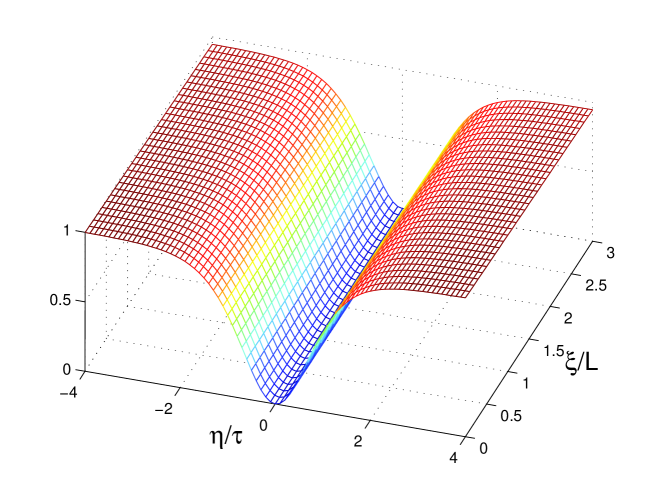
Figure 2: Surface plot of the amplitude for the generated fundamental dark soliton $\left|\Omega_{p}/\Omega_{p0}\right|^{2}\mbox{exp}(-2\alpha\xi)$ with $\left|\Omega_{p}\right|^{2}$ being the numerical solution to Eq. (15) versus dimensionless time $\eta/\tau$ and distance $\xi/L$ under the initial condition $\Omega_{p}(\xi=0,\eta)=\Omega_{p0}\mbox{tanh}^{2}(\eta/\tau)$, where $L=1.0$ cm, $\tau=1.0\times 10^{-6}$s, and other simulation parameters are explained in the main text.

Our scheme is different from EIT in a SQW structure, in which the latter can not form solitons. Because that slow group velocity propagation requires weak driving conditions, this leads to very narrow transparency windows. Thus EIT operation with weak driving conditions requires single and two-photon resonance excitations, i.e., $\Delta_{1}=\Delta_{2}=0$ in Eq. (17). Deviations from these conditions will result in significant probe field attenuation and distortion. Besides, one can find that the nonlinear coefficient $W$ is almost purely imaginary under these EIT conditions. This is contradictory to the requirement of $W\simeq W_{r}$ in order to preserve the complete integrability of the standard nonlinear Schrödinger Eq. (19). However, here we have found that by appropriately choosing the intensities and detunings of laser fields, we can achieve $\mbox{exp}(-\alpha L)\simeq 1$ for $L$ within a few centimeters, $K_{2}\simeq K_{2}r$, $W\simeq W_{r}$, and ultraslow group velocities for both bright and dark solitons studied in this work with the typical population decay and dephasing decay rates of the transitions in SQW structures. Considering a system where the total decay rates are $\gamma_{2}=\gamma_{3}=5\mbox{meV}$, the parameters used are typical values for transitions $\left|1\right\rangle\leftrightarrow\left|2\right\rangle$ and $\left|2\right\rangle\leftrightarrow\left|3\right\rangle$ in SQW structures.

As an example, we now present numerical examples to demonstrate the existence of ultraslow dark solitons in the system studied through simulating the Eq. (15) with the initial condition $\Omega_{p}(\xi=0,\eta)=\Omega_{p0}\mbox{tanh}(\eta/\tau)$. Take $\epsilon_{12}=80\mbox{cm}^{-1}\mbox{meV}$, $\Omega_{c}=8\mbox{meV}$, $\Delta_{1}=-10\mbox{meV}$, $\Delta_{2}\simeq 0$, and $\gamma_{2}=\gamma_{3}=5\mbox{meV}$, we have $V_{g}/c\simeq 2.7\times 10^{-4}$, and $\alpha\simeq 0.00019\mbox{cm}^{-1}$. With these parameters, the standard nonlinear Schrodinger equation (19) with $K_{2r}\cdot W_{r}<0$ is well characterized, and thus we have demonstrated that the existence of dark solitons that travel with ultraslow group velocities in SQW structures. As shown in Fig. 2, the numerical simulation of Eq. (15) for the fundamental dark soliton shows an excellent agreement with Eq. (20).

It is worth to note that all the parameter sets also lead to negligible loss of the probe field for both the bright and dark solitons (including 2-soliton) described here. Besides, we have used the one-dimensional model in calculation where the momentum-dependency of subband energies has been ignored. However, there is no large discrepancy between the reduced one-dimensional calculation [13] and the full two-dimensional calculation [19, 29].

In conclusion, using the coupled Schrödinger-Maxwell equations for a three-level system of electronic subbands, we have presented and analyzed a novel scheme to achieve ultraslow bright and dark optical solitons, and a large XPM phase shift can also be obtained with appropriate parameters. Such investigations of ultraslow optical solitons in the present work may lead to important applications including high-fidelity optical delay lines and optical buffers in SQW structures. Besides, a large XPM phase shift achieved in our proposed SQW structure may open up an avenue to explore possibilities for nonlinear optics and quantum information processing in a solid-state system and may result in substantial impacts on technology of electrically controlled phase modulator.