Chemical Abundances and Dust in Planetary Nebulae in the Galactic Bulge

Abstract

We present mid-infrared Spitzer spectra of eleven planetary nebulae in the Galactic Bulge. We derive argon, neon, sulfur, and oxygen abundances for them using mainly infrared line fluxes combined with some optical line fluxes from the literature. Due to the high extinction toward the Bulge, the infrared spectra allow us to determine abundances for certain elements more accurately that previously possible with optical data alone. Abundances of argon and sulfur (and in most cases neon and oxygen) in planetary nebulae in the Bulge give the abundances of the interstellar medium at the time their progenitor stars formed; thus these abundances give information about the formation and evolution of the Bulge. The abundances of Bulge planetary nebulae tend to be slightly higher than those in the Disk on average, but they do not follow the trend of the Disk planetary nebulae, thus confirming the difference between Bulge and Disk evolution. Additionally, the Bulge planetary nebulae show peculiar dust properties compared to the Disk nebulae. Oxygen-rich dust feature (crystalline silicates) dominate the spectra of all of the Bulge planetary nebulae; such features are more scarce in Disk nebulae. Additionally, carbon-rich dust features (polycyclic aromatic hydrocarbons) appear in roughly half of the Bulge planetary nebulae in our sample, which is interesting in light of the fact that this dual chemistry is comparatively rare in the Milky Way as a whole.

1. Introduction

Abundances of planetary nebulae (PNe) have long been used to aid in the understanding of the chemical history of the Milky Way. Certain elements such as argon and sulfur (and neon as long as the initial mass is not near 3 $M_{\odot}$ and oxygen if initial mass of the progenitor star is $\lesssim 5M_{\odot}$, Karakas & Lattanzio 2003; Karakas 2003) are not changed in the course of the evolution of the low and intermediate mass precursor stars of PNe. Thus the abundances of these elements give the chemical composition of the cloud from which the PNe progenitor stars formed. Many abundance studies have been made of PNe (as well as stars and H II regions) in the Galactic Disk, leading to the determination of abundance gradients across the Disk (e.g. Shaver et al., 1983; Rolleston et al., 2000; Pottasch & Bernard-Salas, 2006). However, due to the high extinction toward the Bulge, there is a relative paucity of abundance studies of PNe as well as stars and H II regions in the Bulge.

Galactic bulges and spheroids may contain half of the stars in the local universe (Ferreras et al., 2003). Thus, understanding their chemical evolution and formation is important to a general theory of galaxy formation. Insights into our own Galactic Bulge formation have implications for bulge formation in general.

Abundances of Galactic Bulge planetary nebulae (GBPNe) have the potential to answer questions about how the Bulge formed. For example, what type of collapse formed the Bulge (dissipational or dissipationless)? And, has secular evolution within the Galaxy since Bulge formation caused a significant amount of star formation within the Bulge (Minniti et al., 1995)? At a bare minimum, a difference between abundance gradients of PNe in the Bulge and Disk would imply that they formed in separate processes.

The large extinction toward the GBPNe makes infrared (IR) lines preferable to optical lines for determining their abundances. Additionally, infrared lines provide essential data on important ionization stages of argon, neon, and sulfur as well as O IV for oxygen. We complement the IR data with optical data where necessary, so that we need no or only small ionization correction factors (ICFs) to account for unobserved stages of ionization. Finally, abundances derived from IR lines depend only weakly on the electron temperature (Rubin et al., 1988; Pottasch & Beintema, 1999). All of these factors lead to more accurately determined abundances than previously possible with optical lines alone. Likewise, IR spectra are well suited to study the various dust features of GBPNe because signatures of both oxygen-rich dust (in the form of crystalline silicates) and carbon-rich dust (in the form of polycyclic aromatic hydrocarbons; PAHs) can be observed if they are present.

Abundances for a number of Galactic Disk planetary nebulae (GDPNe) were determined with the use of spectra taken with the Infrared Space Observatory (ISO; e.g. Pottasch & Bernard-Salas, 2006). However, ISO lacked the sensitivity to study PNe further than 3–4 kpc away from the Sun. As a result, ISO only studied two Bulge PNe, M1-42 and M2-36. Due to the better sensitivity of the Infrared Spectrograph (IRS; Houck et al., 2004) on the Spitzer Space Telescope (Werner et al., 2004) we are able to obtain spectra of GBPNe closer to the Galactic Center; the furthest GBPN in our sample is about 10 kpc from the Sun.

In this paper we present Spitzer IRS spectra of eleven GBPNe. The next section describes the Spitzer data, while §3 describes the supplementary data we use. In §4 we describe the data analysis, deriving ionic and total abundances of argon, neon, sulfur, and oxygen. Additionally we identify the crystalline silicate features and measure PAH fluxes. Finally we discuss what our results imply for the evolution of the Galactic Bulge and its PNe in §5 and conclude in §6.

2. Spitzer IRS Data

2.1. Observations

We observed eleven GBPNe with the Spitzer IRS between September 2006 and September 2007 as part of the Guaranteed Time Observation program 30550. In order to minimize slit losses, PeakUp with 0.4″ positional accuracy was performed for the six PNe where it was possible, while blind pointing with $\sim$1″ positional accuracy was done for the remaining five PNe. We observed these PNe with the IRS Short-Low (SL), Short-High (SH), and Long-High (LH) modules, covering the wavelength range from 5 to 40 µm. In order to subtract the background and minimize the effect of rogue pixels, we took off-source observations for SH and LH; for the SL module we subtracted the background by differencing the orders. The data were taken in staring mode so that spectra were obtained at two nod positions along each IRS slit. For SH and LH, a short exposure time of six seconds was used to keep the bright lines from saturating, with a total of four cycles for redundancy and to aid in the removal of cosmic rays; for the SL module, data were taken in three cycles of fourteen seconds each. Table 1 gives the object names, their Astronomical Observation Request (AOR) keys and coordinates.

2.2. Source Selection

The sources were selected to ensure they belong to the Bulge according to the following criteria. (1) Foremost, the best criterion for ensuring Bulge membership is having galactic coordinates $|\ell|<10\arcdeg$ and $|b|<10\arcdeg$ (Pottasch & Beintema, 1999). All of the sources were selected to meet this criterion. (2) We selected objects with high radial velocities, except for two objects, PNG001.6-01.3 and PNG002.1+03.3, where they are unknown and whose IRAS fluxes and positions indicate that they are members of the Bulge, (Acker et al., 1992). (3) Finally, the objects have diameters $\lesssim$ 5″. Pottasch & Beintema (1999) consider all PNe with diameters $>$ 12″ to be foreground objects, and thus choosing small diameters helped to ensure Bulge membership. Table 1 gives the radial velocities and diameters of our GBPNe.

Additionally, in order to make certain that we could get good Spitzer IRS spectra of the GBPNe, we chose isolated objects in the IRAS Point Source Catalog (PSC) with small radial extent, accurate coordinates, and observable intensities. While the IRAS PSC is not as sensitive as our Spitzer observations (the IRAS PSC catalog is sensitive to a couple hundred mJy whereas our Spitzer observations are sensitive to a few mJy), we check that only one source is on the slit during the data reduction. The criterion of selecting PNe with small sizes also ensured that nearly all of the flux from most of the PNe could be observed within SL, the smallest IRS slit at 3.6″ across. The sources also were chosen to have coordinates known to better than 1.4″ from the radio positions of Condon & Kaplan (1998), and these coordinates were refined with the 2MASS catalog. Finally, we chose objects with radio fluxes at 21 cm (F_21cm) that implied IR fluxes bright enough (F_21cm $>$ 10 mJy) to allow for short integration times, but dim enough (F_21cm $<$ 50 mJy) to not saturate any of the IRS modules. Table 1 gives the IRAS fluxes at 12 and 25 µm as well as the radio fluxes at 21 cm for our objects.

2.3. Data Reduction

We start with basic calibrated data (bcd) from the Spitzer Science Center’s pipeline version s15.3 or s16.1, and run it through the IRSCLEAN program to remove rogue pixels, which uses a mask of rogue pixels from the same campaign as the data. Then we take the mean of repeated observations (cycles) to improve the signal to noise ratio. After that the background is subtracted using the off-source positions for SH and LH, and using the off-order for SL (for example, SL1 nod1 - SL2 nod1). Next we use SMART (Higdon et al., 2004) to manually extract the images, using full-slit extraction for SH and LH and variable-column extraction for SL; we also inspect the spectral profiles of each target with the Manual Source Finder tool in SMART to ensure that only one source is within the slit. Spikes due to deviant pixels which the IRSCLEAN program missed are removed manually in SMART. In order to account for flux that fell outside of the IRS slits (due either to a slight mispointing and/or the extended size of the GBPNe), we apply multiplicative scaling factors to each order and nod. The highest flux in LH sets the scaling because LH is large enough to contain the entire flux of all of our GBPNe. Thus, one nod in LH is scaled to the other, the SH nods are then scaled to LH, and the SL nods and orders are then scaled to match SH. Table 2 gives the scaling factors; they are usually quite small ($\leq$1.20) except for three PNe where the scaling factors in SL (the aperture with the smallest width) reach up to 1.70. Figure 1 plots the scaled and nod-averaged spectra. We predict the 12 and 25 µm IRAS fluxes from these scaled IRS spectra and find generally good agreement with the actual IRAS fluxes, confirming that only the IRAS source is within the IRS slit. Finally we use the gaussian profile fitting routine in SMART to measure line fluxes for each nod position of the scaled spectra. Table 3 gives the observed nod-averaged line fluxes. Uncertainties on the line fluxes are usually $\leq$10%, with uncertainties greater than this marked in the table. A less-than sign in Table 3 indicates a 3$\sigma$ upper limit obtained from the instrument resolution and the root mean square (RMS) deviation in the spectrum at the wavelength of the line.

Table 1Basic data for observed GBPNe

PNG	On Position			Off Position	log(FHβ)	R⊙,PN	RGC	Vrad	Diam	IRAS Fluxes (Jy)		F6cm	F21cm
Number	AORkey	RA	DEC	AORkey	(erg cm-2 s-1)	(kpc)	(kpc)	(km s-1)	(″)	F12μm	F25μm	(mJy)	(mJy)
000.7+03.2	17646848	17 34 54.71	-26 35 56.9	17650176	-13.40 $\pm$ 0.20	7.01	1.0$\pm$2.9	-175	5.2	$<$2.01	2.01	15	15.6
000.7+04.7	17647616	17 29 25.97	-25 49 07.1	17650432	-13.90 $\pm$ 0.30	…	$<$4	+40	2.7	0.50	6.56	27.7	12.8
001.2+02.1	17648896	17 40 12.84	-26 44 21.9	17650688	-13.73 $\pm$ 0.10	6.64	1.4$\pm$2.8	-172	4.0	2.19	3.00	26	24.2
001.4+05.3	17647872	17 28 37.63	-24 51 07.2	17650944	-12.70 $\pm$ 0.30	7.90	0.2$\pm$1.9	+42	5.0	$<$0.28	2.71	13	13.8
001.6-01.3	17649152	17 54 34.94	-28 12 43.3	17651200	-13.90 $\pm$ 0.30	…	$<$4	…	4.5	$<$3.41	3.49	…	19.7
002.1+03.3	17649408	17 37 51.14	-25 20 45.2	17651456	…	…	$<$4	…	4.8	$<$1.93	1.71	5	46.0
002.8+01.7	17649664	17 45 39.81	-25 40 00.6	17651712	-13.48 $\pm$ 0.10	7.50	0.6$\pm$2.5	+164	3.8	…	…	…	13.8
006.0-03.6	17648128	18 13 16.05	-25 30 05.3	17651968	-12.11 $\pm$ 0.02	4.91	3.2$\pm$2.1	+136	5.1	$<$1.45	3.35	51	41.2
351.2+05.2	17648384	17 02 19.07	-33 10 05.0	17652224	-12.10 $\pm$ 0.10	7.69	1.2$\pm$1.2	-128	5.0	0.55	1.70	12	14.4
354.2+04.3	17648640	17 14 07.02	-31 19 42.6	17652480	-12.62 $\pm$ 0.10	10.71	2.8$\pm$4.0	-75	4.0	$<$0.34	1.40	9.1	11.6
358.9+03.2	17647104	17 30 43.82	-28 04 06.8	17652736	-13.03 $\pm$ 0.10	5.12	2.9$\pm$2.2	+190	4.0	$<$2.70	3.70	32	27.3

Table 2Multiplicative scaling factors for GBPNe spectra

PNG Number	LHn1	LHn2	SHn1	SHn2	SL1n1	SL1n2	SL3n1	SL3n2	SL2n1	SL2n2
000.7+03.2	1.00	1.00	1.00	1.00	1.00	1.00	1.00	1.00	1.00	1.00
000.7+04.7	1.02	1.00	1.00	1.00	1.00	1.00	1.00	1.00	1.00	1.00
001.2+02.1	1.02	1.00	1.00	1.05	1.00	1.00	1.00	1.00	1.00	1.00
001.4+05.3	1.03	1.00	1.15	1.17	1.15	1.15	1.00	1.15	1.00	1.00
001.6-01.3	1.05	1.00	1.15	1.15	1.15	1.15	1.50	1.50	1.50	1.50
002.1+03.3	1.00	1.00	1.20	1.20	1.20	1.20	1.20	1.20	1.20	1.20
002.8+01.7	1.01	1.00	1.05	1.10	1.10	1.10	1.10	1.15	1.10	1.10
006.0-03.6	1.02	1.00	1.15	1.15	1.15	1.15	1.60	1.70	1.50	1.40
351.2+05.2	1.02	1.00	1.15	1.15	1.50	1.50	1.50	1.40	1.50	1.40
354.2+04.3	1.02	1.00	1.15	1.15	1.20	1.20	1.20	1.20	1.20	1.20
358.9+03.2	1.02	1.00	1.12	1.10	1.15	1.15	1.00	1.20	1.00	1.00

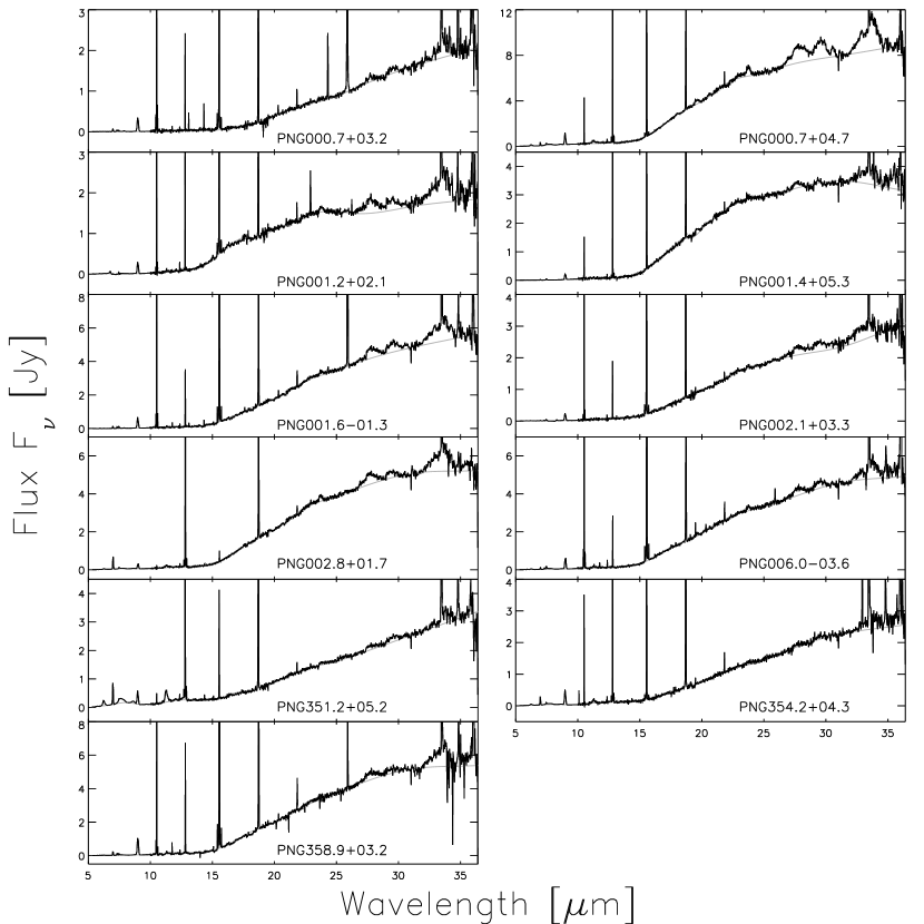
Figure 1.— Scaled, nod-averaged Spitzer IRS spectra (black) of our GBPNe. SL data is presented below 10 µm, and HR data above 10 µm. The spline-fits to the continua (which we subtract from the spectra later in order to better view the crystalline silicate features) is over-plotted (grey).

Table 3Observed infrared line fluxes

Line	$\lambda$	Observed line fluxes for each object labeled by PNG number (10-14 erg cm-2 s-1)
	µm	000.7+03.2	000.7+04.7	001.2+02.1	001.4+05.3	001.6-01.3	002.1+03.3	002.8+01.7	006.0-03.6	351.2+05.2	354.2+04.3	358.9+03.2
$[$Ar II$]$	6.99	26.15	111.62	$<$8.53	6.63	51.51	$<$4.80	253.42	35.44	304.57	92.77	85.93
H I(6-5)+	7.46	13.47	36.22	22.15	19.40	49.27	18.57	31.19	61.70	28.02	19.67	38.81
$[$Ar V$]$	7.90	8.82	$<$13.74	$<$2.95	$<$2.26	$<$12.65	$<$5.38	$<$7.96	$<$10.93	$<$14.98	$<$8.17	$<$9.49
$[$Ar III$]$	8.99	162.55	397.33	124.24	90.22	278.81	100.22	108.59	260.64	173.77	192.54	472.17
$[$S IV$]$	10.52	1401.40	186.81	573.91	67.45	1882.50	688.40	10.42	2179.00	19.77	182.90	1593.55
H I(7-6)+	12.37	5.35	14.18	10.53	6.70	9.37	7.37	11.16	17.13	8.10	7.58	11.89
$[$Ne II$]$	12.82	88.21	1414.80	133.51	408.05	142.14	72.09	1188.85	106.01	1132.05	687.65	228.45
$[$Ar V$]$	13.10	14.98	$<$3.69	$<$3.30	$<$5.12	9.25	$<$4.47	$<$4.73	$<$4.35	$<$3.90	$<$4.25	$<$3.75
$[$Ne V$]$	14.32	22.06	$<$3.09	$<$2.40	$<$2.61	11.74	$<$2.63	$<$3.63	$<$2.85	$<$4.62	$<$3.51	$<$3.52
$[$Ne III$]$	15.56	1590.25	1466.85	1500.55	333.59	3669.75	1313.55	17.82	3455.80	126.08	676.02	5245.25
$[$S III$]$	18.73	419.10	503.54	344.60	333.46	737.29	255.92	601.26	669.36	795.01	600.36	866.11
$[$Ar III$]$	21.84	11.03	22.48	8.10	7.01	22.43	5.91	12.44	20.29	9.27	11.78	34.77
$[$Ne V$]$	24.30	30.29	$<$8.73	$<$2.71	$<$3.18	8.63	$<$2.40	$<$4.78	$<$4.50	$<$2.55	$<$3.06	$<$8.33
$[$O IV$]$	25.91	3580.55	$<$8.83	$<$2.63	$<$3.83	1313.85	$<$2.42	$<$4.52	16.94	$<$3.33	$<$2.85	101.99
$[$S III$]$	33.50	344.92	110.49	190.76	164.33	264.60	158.36	227.22	214.29	499.02	417.67	267.07
$[$Ne III$]$	36.03	181.76	121.71	150.23	$<$36.43	350.23	110.85	$<$25.80	283.73	$<$29.97	70.92	401.05

3. Supplementary Data

Table 4Extinction corrected optical line fluxes

Line	$\lambda$	Extinction corrected line fluxes relative to H$\beta$=100 for each object labeled by PNG number
	Å	000.7+03.2	000.7+04.7	001.2+02.1	001.4+05.3	001.6-01.3	002.8+01.7	006.0-03.6	351.2+05.2	354.2+04.3	358.9+03.2
$[$O II$]$	3727	114.0	…	…	…	…	…	55.13	59.60	130.0	…
$[$Ne III$]$	3869	69.6	…	32.86	…	…	…	95.19	…	9.70	…
$[$O III$]$	4363	12.4	2.81	…	…	…	…	6.68	…	…	…
$[$Ar IV$]$+He I	4712	7.00	…	…	…	…	…	1.91	…	…	…
$[$Ar IV$]$	4740	4.61	…	…	…	…	…	1.93	…	…	…
$[$O III$]$	4959	279.1	123.99	231.9	118.2	354.2	…	369.54	7.27	46.41	339.1
$[$O III$]$	5007	790.4	360.37	728.0	304.7	1003.8	22.65	1067.55	25.89	136.5	989.4
$[$S III$]$	6312	1.86	1.37	1.34	0.71	…	…	2.08	…	1.01	2.02
$[$S II$]$	6717	13.35	2.76	2.77	2.70	6.40	4.77	4.35	6.46	5.96	6.68
$[$S II$]$	6731	19.47	5.12	4.37	3.30	14.38	9.06	7.83	9.31	9.36	12.41
$[$Ar V$]$	7005	0.67	…	…	…	…	…	…	…	…	…
$[$Ar III$]$	7135	30.79	29.22	15.79	12.24	21.54	6.56	16.15	4.86	9.34	30.66
$[$Ar IV$]$	7236	…	0.96	…	…	…	…	…	…	…	…
$[$Ar IV$]$	7264	…	1.06	…	…	…	…	…	…	…	…
$[$O II$]$	7325	5.15	11.42	7.10	8.33	…	3.87	6.29	0.91	2.07	7.73

We supplement our IR data with optical and radio data from the literature to aid abundance determinations for three reasons. First, we use the observed H$\beta$ and 6 cm radio fluxes to derive the extinction toward GBPNe. Table 1 gives these fluxes from the Strasbourg-ESO Catalogue of Galactic Planetary Nebula (Acker et al., 1992). Second, we adopt electron temperatures derived from ratios of optical line fluxes (discussed in §4.1.2). Third, we use optical line fluxes for ions not observable in our IR spectra (specifically lines fluxes of Ar IV, S II, O II, and O III) to reduce the need for ICFs. (As an aside, no UV line data for any of the GBPNe in our sample are available due to the large extinction toward the Bulge.) When the optical line fluxes are given as observed line fluxes, we apply the logarithmic extinction at H$\beta$ (C_Hβ) given in the paper to correct the lines for extinction because it gives the correct Balmer decrement. When more than one paper gives a value for a line flux, we take the average (after correcting all line fluxes for extinction), and Table 4 gives the optical extinction corrected line fluxes adopted for the calculation of abundances.

All of the PNe in this sample should be within $\sim$4 kpc or less of the Galactic Center because they were selected to be members of the Bulge. In order to determine approximately where they are within the Bulge to place them on a plot of abundance versus galactocentric distance, we adopt the heliocentric statistical distances from Zhang (1995). We chose these distances because Zhang (1995) lists distances to more of our objects than other studies, such as van de Steene & Zijlstra (1995) and Cahn et al. (1992). An accurate statistical distance scale for PNe is difficult to obtain, and controversies exist as to which statistical distance scales are the best: for example Bensby & Lundström (2001) find that Zhang’s distance scale is good, while Ciardullo et al. (1999) find that it is not as good. However, regardless of which statistical distances we adopt, the conclusions of the paper will remain unchanged because all of the PNe in our sample are constrained to be in the Bulge by other criteria and we include the large uncertainties that go with these statistical distances in the data analysis.

We adopt the distance from the Sun to the Galactic Center, R_o, from Reid (1993) who determines the best estimate of this distance by taking a weighted average of the various determinations of R_o from different methods. Reid (1993) finds that R${}_{\rm o}=8.0\pm 0.5$ kpc, and this value seems to agree with more current estimates of this distance (e.g. López-Corredoira et al., 2000; Eisenhauer et al., 2005; Groenewegen et al., 2008). Galactocentric distances (R_GC) are then calculated assuming this R_o, and uncertainties on R_GC are calculated using standard error propagation and assuming an uncertainty of 40% on the heliocentric distance (Zhang 1995 estimates the accuracy of the PN distance scale as 35-50% on average). If the distance to a PN is unknown, we assume it is within 4 kpc of the Galactic Center. Table 1 lists the heliocentric and galactocentric distances for each object.

4. Data Analysis

4.1. Abundances

Before determining abundances for this sample of GBPNe, we must first calculate and then correct for extinction. Additionally we adopt electron temperatures (T_e) from the literature and then employ infrared line ratios to derive the electron densities (N_e). After that we use the values of the above quantities to obtain abundances for each ion. The following subsection discuss the details of the calculations of extinction, the selection of T_e and N_e, and finally the derivation of ionic and total abundances.

4.1.1 Extinction Correction

We first calculate the reddening correction by comparing the H$\beta$ flux predicted from IR hydrogen recombination lines to the observed H$\beta$ flux (see Table 5). In order to predict the H$\beta$ flux from the IR H I lines, we adopt the theoretical ratios of hydrogen recombination lines from Hummer & Storey (1987) and assume case B recombination for a gas at T_e= 10⁴ K and N_e= 10³ cm^-3. The H I(7-6) line at 12.37 µm and the H I(11-8) line at 12.39 µm are blended in the SH spectrum, and theoretically the H I(7-6) line contributes 89% of total line flux. Similarly, nearby lines of H I(6-5), H I(17-8), H I(8-6), and H I(11-7) contribute to the H I line at 7.46 µm, with the H I(6-5) flux theoretically contributing 74% of the total line flux. The contributions of additional lines are removed before calculating the predicted H$\beta$ flux from the H I(7-6) and H I(6-5) IR lines.

Additionally we calculate extinction by comparing the H$\beta$ flux predicted from the radio flux at 6cm to the observed H$\beta$ flux. We assume that T_e=$10^{4}$ K (and thus t $\equiv$ T_e/$10^{4}$ K = 1), He⁺/H⁺=0.09, and He⁺⁺/H⁺=0.03 and use the following formula from Pottasch (1984):

$${F(H\beta)}_{6cm}^{predicted}={S_{6cm}\over 2.82\times 10^{9}t^{0.53}(1+{He^{+}/H^{+}}+3.7{He^{++}/H^{+}})}$$

where $2.82\times 10^{9}$ converts units so that $S_{6cm}$ is in Jy and F(H$\beta$) is in erg cm^-2 s^-1. Table 1 gives the values for $S_{6cm}$ and F(H$\beta$) while Table 5 gives the calculated values of the extinction.

For the abundance calculations, in order to weight the extinctions calculated from both of the above methods equally, we use

$${C_{H\beta,final}=\frac{C_{H\beta,HI(7-6)}}{4}+\frac{C_{H\beta,HI(6-5)}}{4}+\frac{C_{H\beta,radio}}{2}}$$

when we have extinctions from both H I lines and the radio, otherwise we just take an average (see Table 7 for these adopted values). There is no H$\beta$ flux available for PNG002.1+03.3 and thus we adopt an extinction to it from the average of the other GBPNe extinctions. Table 5 gives the extinction values derived here along with those from the literature. In general there is very good agreement between the different methods.

We use the extinction law from Fluks et al. (1994) and assume the standard $R_{V}$ of the Milky Way of 3.1. However, there is evidence that interstellar extinction is steeper than this toward the Bulge, e.g. Walton et al. (1993) find that $R_{V}$=2.3 and Ruffle et al. (2004) find $R_{V}$ = 2.0. Nevertheless, abundances determined from IR lines are not greatly affected by this change in $R_{V}$: an $R_{V}$=2.0 usually changes their abundances by $\lesssim$5% (and at most 10%) compared to the usual $R_{V}$=3.1. Thus, because the previous optical studies to which we compare assumed R_V=3.1, and because the IR lines are even less affected by the choice of R_V, we assume R_V=3.1.

Table 5Comparison of the derived C_Hβ  with the literature

PNG	This work			ARKS91	RPDM97		CMKAS00	ECM04	WL07		TASK92
Number	H I(7-6)	H I(6-5)	6 cm	Balmer	Balmer	6 cm	Balmer	H$\alpha$/H$\beta$	H$\alpha$/H$\beta$	6 cm	Balmer	6 cm
000.7+03.2	2.10	2.00	2.05	2.17	2.35	2.26	2.11	…	…	…	2.2	2.0
000.7+04.7	3.02	2.93	2.81	3.33	…	…	…	2.88	…	…	3.3	2.8
001.2+02.1	2.72	2.55	2.62	2.71	…	…	…	2.40	…	…	2.7	2.6
001.4+05.3	1.50	1.46	1.28	1.25	…	…	1.45	…	…	…	1.36	1.3
001.6-01.3	2.84	3.06	…	3.35	…	…	…	…	…	…	3.4:	…
002.1+03.3	…	…	…	…	…	…	…	…	…	…	…	…
002.8+01.7	2.50	2.45	…	3.07	…	…	…	…	…	…	3.1	…
006.0-03.6	1.31	1.37	1.29	…	1.43	1.35	…	…	1.41	1.18	1.30	1.32
351.2+05.2	0.98	1.02	0.65	1.11	0.985	0.735	…	…	…	…	1.14	0.68
354.2+04.3	1.47	1.39	1.05	1.69	1.78	…	…	…	…	…	1.67	1.08
358.9+03.2	2.08	2.09	2.01	2.22	2.23	2.15	2.29	…	…	…	2.2	2.04

4.1.2 Electron Temperature and Density

In order to derive abundances, we adopt two electron temperatures (T_e): T[N II] for the low-ionization potential ions (Ar II, Ne II, S II, and O II), and T[O III] for the high-ionization potential ions. Table 6 gives the electron temperatures from the literature. When possible, our adopted T[N II] and T[O III] are an average of the values from the literature. If temperatures are not available in the literature, we assume the average value from the other GBPNe in the sample ($<$T[N II]$>$ = 8100 K and $<$T[O III]$>$ = 10700 K). Abundances from IR lines depend only weakly on the adopted T_e, and thus our assumption does not strongly affect our abundances — especially those of argon, neon, and sulfur which are mostly determined from IR lines.

We determine electron densities (N_e) from IR line ratios of S III, Ne III, Ar III, Ar V, and Ne V (see Table 6). The S III line ratio gives the best estimate of N_e, and thus we adopt it for the abundance analysis. Densities determined from the other line ratios are more uncertain because they either rely on at least one line with a weak flux, or the density is outside the range of what the line ratio can accurately measure. The adopted N_e from the S III ratios have an average of 3500 cm^-3, and range from 1000 to 9200 cm^-3.

Table 6Electron Temperatures and Densities

PNG	Temperature Te (K)		Density Ne (cm-3)
Number	[O III]	[N II]	[S III]	[Ne III]	[Ar III]	[Ar V]	[Ne V]
000.7+03.2	10200, 13300	8000, 8400	1000	low	120	370	low
000.7+04.7	10200, 10200	8500	9200	3100	10000	…	…
001.2+02.1	10200	…	2100	low	2000	…	…
001.4+05.3	10200	8300	2500	…	low	…	…
001.6-01.3	…	…	4700	low	500	…	3000
002.1+03.3	…	…	1700	2200	7500	…	…
002.8+01.7	10200	…	3900	…	low	…	…
006.0-03.6	9800, 9840	9300, 11370	5000	3600	low	…	…
351.2+05.2	10200, 9300	7000:, 6000	1700	…	14000	…	…
354.2+04.3	10200	6600, 6400	1400	low	5400	…	…
358.9+03.2	10200, 7700, 10400	8300, 8200, 8900	5300	7700	low	…	…

4.1.3 Ionic and Total Abundances

Table 7Adopted parameters for determining abundances

PNG	F${}_{H_{\beta},predicted}$	C${}_{H_{\beta}}$	Ne	T$[$O III$]$	T$[$N II$]$
Number	(10-14 erg cm-2 s-1)		(cm-3)	(K)	(K)
000.7+03.2	483	2.05	1000	11800	8200
000.7+04.7	1328	2.89	9200	10200	8500
001.2+02.1	902	2.62	2100	10200	8100
001.4+05.3	630	1.38	2500	10200	8300
001.6-01.3	1280	2.95	4700	10700	8100
002.1+03.3	662	1.87	1700	10700	8100
002.8+01.7	1071	2.47	3900	10200	8100
006.0-03.6	1791	1.32	5000	9800	10300
351.2+05.2	816	0.82	1700	9800	6500
354.2+04.3	674	1.23	1400	10200	6500
358.9+03.2	1211	2.04	5300	14200	8500

Table 8Ionic Abundances

Ion	x	$\lambda$	Ionic abundances for each object labeled by PNG number
			000.7+03.2	000.7+04.7	001.2+02.1	001.4+05.3	001.6-01.3	002.1+03.3	002.8+01.7	006.0-03.6	351.2+05.2	354.2+04.3	358.9+03.2
Ar+	-7	6.99	5.97	9.39	$<$1.07	1.14	4.63	$<$0.81	26.90	1.74	47.20	17.60	7.69
Ar+2	-7	8.99	39.60	42.00	17.90	16.60	29.50	18.30	13.30	17.70	24.00	32.30	43.70
Ar+2	-7	21.8	35.10	34.70	15.30	18.40	31.80	14.40	20.70	20.60	18.60	27.80	44.40
Ar+2	-7	7135	20.70	25.70	13.90	10.80	17.20	…	5.76	15.70	4.71	8.23	14.90
Ar+3 +	-7	4712	11.50	…	…	…	…	…	…	6.88	…	…	…
Ar+3	-7	4740	9.59	…	…	…	…	…	…	5.96	…	…	…
Ar+4	-7	7.88	0.76	$<$0.44	$<$0.14	$<$0.15	$<$0.42	$<$0.34	$<$0.32	$<$0.25	$<$0.77	$<$0.50	$<$0.31
Ar+4	-7	13.1	0.82	$<$0.11	$<$0.10	$<$0.23	0.24	$<$0.19	$<$0.14	$<$0.08	$<$0.13	$<$0.17	$<$0.10
Ne+	-5	12.8	3.14	18.80	2.63	10.80	2.01	1.89	19.70	0.83	25.60	19.10	3.20
Ne+2	-5	15.5	21.80	8.43	11.70	3.59	20.90	13.50	0.12	13.70	1.04	6.67	28.20
Ne+2	-5	36.0	27.70	8.84	13.10	$<$4.54	23.30	12.80	$<$2.00	13.80	$<$2.87	7.97	25.90
Ne+2	-5	3869	3.93	…	3.04	…	…	…	…	10.40	…	0.90	…
Ne+4	-7	14.3	3.89	$<$0.26	$<$0.23	$<$0.35	0.87	$<$0.34	$<$0.31	$<$0.15	$<$0.46	$<$0.42	$<$0.28
Ne+4	-7	24.3	5.22	$<$1.67	$<$0.31	$<$0.54	1.04	$<$0.34	$<$0.61	$<$0.40	$<$0.29	$<$0.39	$<$1.02
S+	-7	6717	14.50	8.22	4.13	4.06	14.40	…	9.66	4.97	18.20	15.40	13.90
S+	-7	6731	18.20	7.86	4.55	3.31	18.60	…	11.00	5.23	18.70	18.40	14.50
S+2	-7	18.7	99.30	77.60	49.20	66.50	88.00	46.90	81.10	57.20	118.00	105.00	94.00
S+2	-7	33.4	92.30	71.10	45.50	62.90	86.50	43.30	75.70	55.10	115.00	99.90	85.10
S+2	-7	6312	25.30	29.90	30.50	16.00	…	…	…	55.10	…	23.10	14.70
S+3	-7	10.5	73.90	5.99	18.80	2.88	50.80	28.00	0.31	38.10	0.61	6.76	38.90
O+	-6	3728	128.00	…	…	…	…	…	…	31.20	279.00	582.00	…
O+	-6	7327	225.00	179.00	261.00	240.00	…	…	113.00	32.90	218.00	534.00	143.00
O+2	-6	4959	174.00	117.00	218.00	111.00	289.00	…	…	401.00	7.88	43.70	130.00
O+2	-6	5007	170.00	118.00	237.00	99.50	284.00	…	7.36	401.00	9.72	44.50	131.00
O+3	-6	25.8	157.00	$<$0.43	$<$0.08	$<$0.18	41.80	$<$0.09	$<$0.16	0.41	$<$0.10	$<$0.10	3.11

Table 9Comparison of Total Elemental Abundances for Individual Bulge PNe

PNG	This work				RPDM97				CMKAS00			ECM04				WL07
Number	Ar	Ne	S	O	Ar	Ne	S	O	Ar	S	O	Ar	Ne	S	O	Ar	Ne	S	O
000.7+03.2	5.2	3.7	1.9	5.1	4.8	0.56	0.62	2.1	7.1	2.0	10.0	…	…	…	…	…	…	…	…
000.7+04.7	5.4	2.7	0.88	3.0	…	…	…	…	…	…	…	4.4	…	0.36	1.9	…	…	…	…
001.2+02.1	2.0	1.5	0.70	4.9	…	…	…	…	…	…	…	1.7	0.35	0.46	3.0	…	…	…	…
001.4+05.3	2.5	1.4	0.71	3.5	…	…	…	…	1.9:	0.56	4.9	…	…	…	…	…	…	…	…
001.6–01.3	4.6	3.2	1.6	3.3	…	…	…	…	…	…	…	…	…	…	…	…	…	…	…
002.1+03.3	1.8	1.5	0.73	…	…	…	…	…	…	…	…	…	…	…	…	…	…	…	…
002.8+01.7	5.3	2.0	0.89	1.2	…	…	…	…	…	…	…	…	…	…	…	…	…	…	…
006.0–03.6	2.8	1.9	0.99	4.3	2.3	1.1	0.85	4.8	…	…	…	…	…	…	…	1.9	0.98	1.3	4.6
351.2+05.2	7.1	2.7	1.4	2.6	2.9	…	2.3	2.2	…	…	…	…	…	…	…	…	…	…	…
354.2+04.3	5.3	2.6	1.3	6.0	3.8	1.6	0.71	7.2	…	…	…	…	…	…	…	…	…	…	…
358.9+03.2	6.5	4.0	1.4	2.8	5.6	5.1	0.36	9.3	3.6:	1.2	6.3	…	…	…	…	…	…	…	…

Figure 2.— Continuum subtracted spectra showing the crystalline silicate features. See Figure 1 for the spline fit to the continuum.

Table 10Net PAH Feature Fluxes

PNG	Net PAH Feature Fluxes ( x 10-20 W cm-2)
Number	6.2µm LR	7.7µm LR	8.6µm LR	11.2µm LR	11.2µm HR	12.7µm HR
000.7+04.7	15.0 $\pm$ 0.2	27.3 $\pm$ 0.6	4.6 $\pm$ 0.2	11.3 $\pm$ 0.2	16.5 $\pm$ 0.8	12.$\pm$ 6.
002.8+01.7	5.3 $\pm$ 0.1	8.4 $\pm$ 0.7	2.49 $\pm$ 0.08	6.08 $\pm$ 0.07	7.6 $\pm$ 0.5	9.$\pm$ 6.
006.0-03.6	4.0 $\pm$ 0.2	11.0 $\pm$ 0.8	2.0 $\pm$ 0.1	4.4 $\pm$ 0.1	7.4 $\pm$ 0.5	4.1$\pm$ 0.5
351.2+05.2	29.0 $\pm$ 0.9	40.8 $\pm$ 0.7	10.0 $\pm$ 0.1	22.0 $\pm$ 0.3	24.0 $\pm$ 0.5	11.$\pm$ 4.
354.2+04.3	5.0 $\pm$ 0.2	8.1 $\pm$ 0.3	2.2 $\pm$ 0.1	6.32 $\pm$ 0.08	7.4 $\pm$ 0.5	7.$\pm$ 4.
358.9+03.2	2.1 $\pm$ 0.3	4.7 $\pm$ 0.6	1.4 $\pm$ 0.2	3.4 $\pm$ 0.2	3.4 $\pm$ 0.8	1.$\pm$ 1.

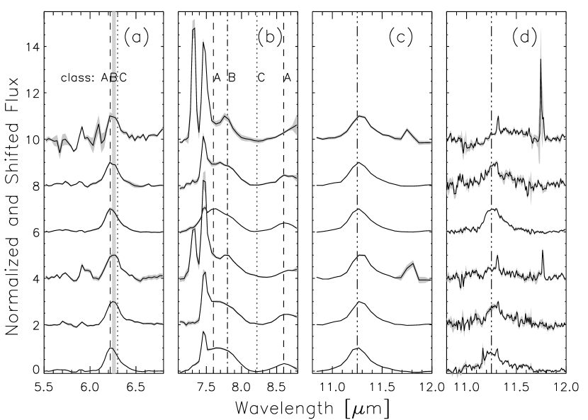
Figure 3.— Profiles of PAH features for PNG358.9+03.2, PNG354.2+04.3, PNG351.2+05.2, PNG006.0-03.6, PNG002.8+01.7, and PNG000.7+04.7 (from top to bottom). (a) Profiles of 6.2 µm  PAHs in LR. The dashed line indicates class A PAHs; the grey shaded area indicates class B; the dotted line indicates class C. (b) Profiles of 7.7 µm  and 8.6 µm  PAHs in LR. The dashed lines indicate class A PAHs; the dot-dashed line, class B; the dotted line, class C. (c) Profiles of 11 µm  PAH in LR. (d) Profiles of 11 µm  PAH in HR.

Table 7 lists the parameters used in determining the PNe ionic abundances. Note that we use a predicted H$\beta$ flux from the IR H I lines in order to ensure that the hydrogen comes from within the same slit as the IR forbidden lines. Table 8 presents the ionic abundances themselves. In order to determine total elemental abundances, the ionic abundances for each element are summed. When the ionic abundance can be determined by more than one line, we choose the abundance(s) from the most reliable line(s), and mark the lines used in Table 8. If necessary, the sum of the ionic abundances for each element is then multiplied by an ionization correction factor (ICF) to account for unobserved ions that are expected to be present. For argon, we apply an ICF for the nine objects for which Ar⁺³ is not observed. For neon, we apply an ICF for the four high ionization nebulae with unobserved Ne⁺³. ICFs are generally small, and we can derive accurate total elemental abundances for many objects, especially for the elements of neon and sulfur whose abundances are derived mainly from IR lines and which rarely need ICFs. Table 9 presents the total elemental abundances.

The Ar⁺³ abundance can only be determined directly from optical lines for two of the GBPNe (PNG000.7+03.2 and PNG006.0-03.6). However, the Ar⁺³ abundance cannot contribute a large amount because the abundance of Ar⁺⁴ always accounts for $<$2% of the total argon abundance. We adopt an ICF to account for unobserved Ar⁺³ determined by Ar⁺³ = 0.28*Ar⁺² because the two GBPNe with observed Ar⁺³ have Ar⁺³/Ar⁺² = 0.27 and 0.29. Additionally, the GDPNe in the sample of Pottasch & Bernard-Salas (2006) for which the ionic abundance of Ar⁺⁴ is less than 2% of the total argon abundance (like our sample of GBPNe) have Ar⁺³/Ar⁺² ranging from 0.15 to 0.68 with a mean of 0.30, so our assumption of Ar⁺³ = 0.28*Ar⁺² is justified.

The Ne⁺³ abundance cannot be determined directly for any of our GBPNe because its lines lie in the UV. However, it is only expected to contribute significantly if the O⁺³ line is detected in the IRS spectrum because its ionization potential (IP=63.45 eV) is near that of O⁺³ (IP = 54.93 eV). The O⁺³ line is detected in only four of the spectra of our GBPNe (PNG000.7+03.2, PNG001.6-01.3, PNG006.0-03.6, and PNG358.9+03.2). Thus, for these four objects only, an ICF is necessary to account for unobserved Ne⁺³. Similarly to Ar⁺³, the Ne⁺³ cannot contribute a huge amount because the abundance of Ne⁺⁴ always accounts for $<$1% of the total abundance of neon. Taking the average of a sample of Galactic PNe, Bernard-Salas et al. (2008) find that Ne⁺³ = 0.35*(Ne⁺² + Ne⁺⁴), and thus we adopt an ICF determined by this to account for unobserved Ne⁺³.

The uncertainties in the derived elemental abundances result from uncertainties in the line fluxes, C_Hβ, T_e, N_e and ICFs. The measured H I line fluxes typically have uncertainties $\lesssim$20%, while the measured fine structure line fluxes usually have uncertainties $\lesssim$10%. Uncertainties are also introduced into the line fluxes from the adopted scaling factors which are typically $\lesssim$15% for the high resolution lines (those lines above 10 µm), but reach 50–70% for the low resolution lines for three objects. However, our scaling factors cannot be far off because the C_Hβ determined from H I lines in in the high and low resolution spectra agree well and the ionic Ar⁺² abundance determined from Ar III lines in the high and low resolution spectra also agree well, even for the nebulae with the largest scaling factors. The uncertainties in C_Hβ and T_e of $\sim$10% each do not have a large affect on the total elemental abundances of argon, neon, and sulfur because these abundances are determined mainly from IR lines; however, they will have a larger affect on the total abundance of oxygen. The uncertainty on N_e is $\sim$30%. The uncertainties on the ICFs for argon and neon are most likely less than a factor of two, causing an abundance uncertainty for these elements of $\lesssim$30% due to the ICFs (when the ICFs are neccessary). A comparison to optically derived abundances for the same objects by various authors gives an estimate of the typical total abundance uncertainty, which is $\sim$50% (e.g. this work, Górny et al., 2004; Bernard-Salas et al., 2008).

4.2. Crystalline Silicates

Crystalline silicate features are present around 28 and 33 µm in the spectra of all GBPNe in our sample, while no amorphous silicate features are observed. In order to illustrate the crystalline silicate features more clearly, we define and subtract a continuum determined by a smooth spline fit to feature-free regions of each spectrum. Figure 1 shows the spline fit to the spectral continua and Figure 2 shows the continuum-subtracted spectra. The spline fit continuum is physically meaningless, and we only use it to elucidate the crystalline silicate features. Following Molster (2000) we identify the 28 micron complex (26.5 – 31.5 µm) and 33 micron complex (31.5 µm to past the end of our spectra) both as having features originating from the magnesium-rich crystalline silicates forsterite (Mg₂SiO₄) and enstatite (MgSiO₃).

The strength of the silicate emission bands can give an approximate estimate of the crystalline dust temperatures. Matsuura et al. (2004) note that the absence of a 23.7 µm feature indicates that forsterite is cooler than 100 K. This feature is either not present or very weak in the spectra of our GBPNe, and thus the forsterite dust in these objects must be cold, with a temperature $\lesssim$100 K.

4.3. PAHs

PAHs are present in six of the eleven GBPNe in our sample: PNG000.7+04.7, PNG002.8+01.7, PNG006.0-03.6, PNG351.2+05.2, PNG354.2+04.3, and PNG358.9+03.2. Absorption of energetic photons excites the PAH emission features at 6.2, 7.7, 8.6, 11.2, and 12.7 µm. PAHs which emit in this spectral range have on the order of tens to hundreds of carbon atoms (Schutte et al., 1993). C—C stretching and bending or deformations causes the 6.2 and 7.7 µm features, while in-plane C—H bending produces the 8.6 µm feature, and out-of-plane C—H bending gives rise to the 11.2 and 12.7 µm features (Allamandola et al., 1989).

Table 10 gives the net integrated PAH fluxes. We calculate these by first subtracting a spline-fit continuum and then summing the remaining flux in each PAH wavelength range; if atomic lines are present, we subsequently subtract their flux to arrive at the net PAH flux. For the 7.7 µm PAH, we subtract the H I line at 7.46 µm (and for PNG006.0-03.6 and PNG358.9+03.2 the 7.32 µm line as well). For the 12.7 µm PAH, we remove the contribution from the Ne⁺ line at 12.81 µm; however, the 12.7 µm PAH is much weaker than the 12.81 µm Ne⁺ line, and thus the net 12.7 µm PAH flux is very uncertain. The 11.29 µm H I is weak and always near the 3-$\sigma$ upper limit in our spectra; it contributes less than 5% to the 11.2 µm PAH flux (except for PNG006.0-03.6 and PNG358.9+03.2 where it may contribute up to 20%) and we do not remove it. Figure 3 shows plots of the continuum-subtracted, normalized PAH profiles.

5. Discussion

5.1. Elemental Abundances

5.1.1 Comparison of Abundances of Individual Objects with the Literature

In Table 9 we compare total elemental abundances from this work with abundances from four papers in the literature: Ratag et al. (1997); Cuisinier et al. (2000); Escudero et al. (2004); Wang & Liu (2007). All of these studies derive total elemental abundances from collisionally excited optical lines, and therefore their abundances are more dependent on the adopted extinction and electron temperature than the current study. A detailed comparison with these studies is hindered by the fact that only one study (Wang & Liu, 2007) lists their ionic abundances and ICFs. For individual objects, our total elemental abundances of argon, neon, and sulfur tend to be higher than the optical abundances. This is due in part to the fact that the IR derived abundances for ions of Ar⁺², Ne⁺² and S⁺² always give a higher ionic abundance than the optically derived abundances for the same ions. On the other hand, the total elemental abundances of oxygen derived here do not have such a systematic offset because the main contributors to the total oxygen abundance, O⁺ and O⁺², are determined from optical line fluxes which are taken from the same literature sources to which we compare abundances; PNG002.1+03.3 does not have an oxygen abundance listed in Table 9 because we could not find any optical line fluxes for this object.

Argon The values for the total argon abundance in this work are systematically higher than the values given in the literature (except in one case where the values are close). Several factors can lead to this offset: (1) In most cases, total elemental argon abundances in this work and prior studies of the GBPNe in our sample must use an ICF to account for unobserved Ar⁺³; different ICFs will lead to different total argon abundances. When the 4740 Å Ar⁺³ line is observed, our elemental argon abundance value agrees to within 30% of the values in the literature. (2) For the low excitation PNe (PNG002.8+01.7, PNG351.2+05.2, and PNG354.2+04.3, Excitation Class, EC$\sim$2–3), the IR data show that Ar⁺ contributes significantly to the total argon abundance, and thus optical studies without observed Ar⁺ must either use an ICF to account for it or risk underestimating the total argon abundance. (3) When we derive the Ar⁺² ionic abundance from the IR lines and the optical 7135 Å line, we always get a value from the IR lines that is higher than that from the optical line (often within 50%, but sometimes off by a factor of a few), which causes many of our IR derived total argon abundances to be systematically higher than those derived in the literature. This may be due to the uncertainty in T_e when using optical lines to derive the Ar⁺² abundance: lowering the electron temperature by 1000 to 2000 K significantly increases the Ar⁺² ionic abundance derived from the optical line (while only slightly increasing the Ar⁺² ionic abundance derived from the IR lines), bringing the optical Ar⁺² abundances into good agreement with the IR Ar⁺² abundances in most cases.

Neon The values for the total neon abundance are systematically higher in this study than in the literature (in all except one case where the values are close). The factors that may cause this are: (1) The IR data show that Ne⁺ is the dominant contributor to the total elemental neon abundance in roughly half of our GBPNe. There is no Ne⁺ line observable in the optical, and thus the optical studies have not observed the most important ionization stage of neon for these PNe. (2) Lines of Ne⁺³ lie in the UV part of the spectrum, and thus our study and previous optical studies must use an ICF to account for it in high ionization nebulae (PNG000.7+03.2, PNG001.6-01.3, PNG006.0-03.6, and PNG358.9+03.2); different assumed ICFs could account for part of the discrepancy for these PNe. (3) When we derive the Ne⁺² ionic abundance from the IR lines and the optical 3869 Å line, we always get a value from the IR lines that is higher than that from the optical. Similarly to Ar⁺², this may be due (at least in part) to the uncertainty in T_e having large affects on the optically derived abundances. Lowering the electron temperature by 1000 to 2000 K increases the Ne⁺² ionic abundance derived from the optical line (while only slightly changing the Ne⁺² ionic abundance derived from the IR lines), bringing the optical and IR derived Ne⁺² abundances into better agreement.

Sulfur Most of the values for our total sulfur abundance are higher than those given in the literature. This is due in part at least to having derived a higher S⁺² abundance from the IR lines as compared to the optical line. The major contributors to the total elemental sulfur abundance are S⁺² and S⁺³, both observed in our IR spectra. The optical S⁺² line at 6312 Å is often weak and quite sensitive to T_e, and S⁺³ is not observed in the optical (Ratag et al., 1997). We use optical lines to determine the abundance of S⁺, but this is not a major contributor to the total sulfur abundance.

Oxygen Our values for the total oxygen abundance usually agree to within a factor of two of those in the literature, and often within 50%. For the one case where we can compare to the study in the literature with published ionic abundances (Wang & Liu, 2007), the ionic abundance of O⁺ is higher by 50% in this work than in that study, but the ionic abundance of O⁺² (the dominant ion) is lower by 10% than in that study, and the total elemental oxygen abundances agree within 10%. The IR data show that for one object (PNG000.7+03.2), the O⁺³ contributes significantly ($\sim$30%) to the total oxygen abundance, and thus optical studies must either use an uncertain ICF or underestimate the total oxygen abundance in this object.

Considering that we employ more observed stages of ionization than purely optical studies and also that we derive ionic abundances for the major contributors to the total elemental abundances for argon, neon, and sulfur from IR lines (which are less sensitive to C_Hβ and T_e than abundances from optical lines), our GBPNe abundances for these elements are more accurate than previous studies. Our GBPNe abundance of oxygen, however, should be of similar accuracy to previous optical studies because we must rely on optical lines for the dominant ionization stages, but we make a slight improvement by measuring or placing an upper limit on the abundance from the O⁺³ infrared line.

5.1.2 Comparison of Mean Abundances with the Literature

We compare our mean Bulge abundance from the GBPNe to mean Bulge abundances derived from other GBPNe abundance studies, red giant stars, and H II regions in Table 11. The mean abundances of our GBPNe generally agree well with mean abundances of GBPNe determined from the optical studies. The mean neon abundances are the most discrepant, with ours being a factor of $\sim$2 higher than those in the literature (reasons for such a discrepancy are given in §5.1.1). Our mean argon and sulfur abundances are within the range of the previous studies, while our mean oxygen abundance is only slightly lower.

Cunha & Smith (2006) derive abundances for seven red giant stars in the Bulge, Lecureur et al. (2007) forty-seven, and Fulbright et al. (2007) twenty-five. Cunha & Smith (2006) derive oxygen abundances from lines of OH vibrational-rotational molecular transitions observed in infrared spectra, while Lecureur et al. (2007) and Fulbright et al. (2007) derive oxygen abundances from the [O I] line at 6300 Å in optical spectra. The oxygen abundances of our GBPNe fall well within the range of values for red giants from these studies, but the mean oxygen abundance of the GBPNe is a factor of $\sim$2 lower than that of the red giants. However, given the uncertainties, small sample size, and different methods used, there is a good agreement.

Simpson et al. (1995) give abundances derived from IR lines for 18 H II regions between 0 and 10 kpc from the Galactic Center, while Martín-Hernández et al. (2002) use ISO spectra to derive abundances of 26 H II regions between 0 and 14 kpc (distances for both studies were redetermined so that R_⊙=8.0 kpc). In order to determine a mean H II region Bulge abundance from these studies, we take the mean of all H II regions in each study within 4 kpc of the Galactic Center. The Bulge H II region abundances from these two studies generally agree well with our GBPNe abundances, but the Bulge oxygen abundance of Simpson et al. (1995) and Bulge argon abundance of Martín-Hernández et al. (2002) are a factor of $\sim$2 higher. There are only 5 objects in the central 4 kpc of Simpson et al. (1995) and only 3 in the central 4 kpc of Martín-Hernández et al. (2002) (and only 11 in our GBPNe sample), and thus the small size of the samples may suggest that the mean does not reflect a true average of the whole Bulge population. Our mean sulfur abundance is the same as that of Martín-Hernández et al. (2002), but over a factor of two smaller than that of Simpson et al. (1995). Interestingly, while our mean GBPNe neon abundance is a factor of $\sim$2 higher than previous GBPNe studies, it agrees very well with the mean Bulge H II region neon abundances from these studies.

In order to compare abundances across the Disk as well as the Bulge of the Galaxy, we supplement our abundances of GBPNe with those of GDPNe that are derived from mainly IR lines in a similar way to the abundances derived in this work. They are mostly from Pottasch & Bernard-Salas (2006) who use chiefly ISO data (excluding the strange low metallicity Hu 1-2), and complemented with abundances of several GDPNe using mainly Spitzer data: NGC 2392 (Pottasch et al., submitted), M1-42 (Pottasch et al., 2007), and IC 2448 (Guiles et al., 2007), and additionally abundances of one PN (NGC 3918) that uses data from IRAS (Clegg et al., 1987). In Table 12 we compare mean abundances of PNe and H II regions with galactocentric distances in the range 0–4 kpc (Bulge), 4–8 kpc (Inner Disk) and beyond 8 kpc (Outer Disk). The abundances from PNe agree reasonably well with the abundances from H II regions derived by Martín-Hernández et al. (2002), but do not agree as well with the abundances from H II regions derived by Simpson et al. (1995). Ratios of abundances of the various $\alpha$-elements to each other (for example, Ne/S, S/Ar, Ne/O) in both PNe and H II regions show flat behavior with galactocentric distance (within the uncertainties), as expected for elements which are thought to be made in the same processes in massive stars.

Table 11Comparison of Mean Bulge Abundances

Study	Ar/H	Ne/H	S/H	O/H
PNe
Current	4.4	2.5	1.1	3.7
RPDM97	3.8	0.98	1.0	5.2
CMKAS00	2.1	…	0.78	5.4
ECM04	4.7	0.75	0.63	3.9
WL07	2.0	1.2	1.1	5.1
Red Giant Stars
CS06	…	…	…	7.3
LHZ07	…	…	…	8.8
FMR07	…	…	…	6.2
H II Regions
SCREH95	…	2.5	2.7	12
MHPM02	7.9	2.4	1.1	…

Table 12Abundances of PNe and H II regions across the Galaxy

Distance range	Ar/H	Ne/H	S/H	O/H
(kpc)
PNe: This work + others (see §5.1.2)
0–4	4.6	2.7	1.2	4.5
4–8	4.3	1.9	1.2	5.0
8–…	2.7	1.1	0.63	4.2
H II Regions: Simpson et al. (1995)
0–4	…	2.5	2.7	12
4–8	…	1.5	1.2	5.6
8–…	…	0.68	0.76	3.6
H II Regions: Martín-Hernández et al. (2002)
0–4	7.9	2.4	1.1	…
4–8	4.7	2.2	0.89	…
8–…	2.6	1.2	0.65	…

5.1.3 Nature of the Bulge

The absence or presence of an abundance gradient in the Bulge (and the magnitude of the gradient if present) gives insight into how the Bulge formed. If the Bulge has an abundance gradient, then it formed by dissipational collapse, where self-enhancement of abundances occurred as the collapse continued inwards. However, if the Bulge does not have an abundance gradient, then it formed by dissipationless collapse, where mergers of small protogalactic pieces caused an inhomogeneous collapse over a long period of time and the mergers mixed stars of different ages and metallicities. If the Bulge has only a shallow abundance gradient, then the gravitational potential of the bar in our Galaxy caused concentrated star formation at its center and the stars eventually left the Disk to become (part of) the Bulge (Minniti et al., 1995).

Several (mainly optical) studies of GBPNe point toward a slightly more metal-rich Bulge than Disk (Ratag et al., 1992; Cuisinier et al., 2000; Górny et al., 2004; Wang & Liu, 2007). However, Ratag et al. (1992) find that the average abundances of GBPNe cannot be predicted by the abundance gradient observed for GDPNe, hinting that stars in the Bulge are a distinct population from the Disk. Additionally, Górny et al. (2004) find that the O/H gradient becomes shallower and may even decrease in the most inner parts of the Disk based on their sample of GDPNe towards the Galactic Center. On the other hand, Exter et al. (2004) find essentially no difference in abundances between their Bulge and Disk PNe samples; however, their results also point to a discontinuation of the Disk metallicity gradient. The large extinction toward the Bulge hinders optical studies of GBPNe. Thus, in this work we seek to confirm the results of the optical studies using mainly infrared data.

In order to discover if the abundance trend in the Disk continues in the Bulge, Figure 4 shows abundances of argon, neon, sulfur, and oxygen versus galactocentric distance for both the GBPNe and GDPNe (GDPNe data discussed in §5.1.2). We fit lines to the plots of GBPNe and GDPNe abundances versus galactocentric distance in this figure separately (excluding from the fit to the oxygen abundance the four GDPNe that are thought to have depleted oxygen due to hot bottom burning, as discussed in Pottasch & Bernard-Salas 2006), and Table 13 gives parameters for these fits. The elemental abundance gradients of the GDPNe range from $-$0.08 to $-$0.14 dex/kpc and have uncertainties of 0.03–0.04 dex/kpc. In Figure 4 we also over plot the oxygen abundance gradient passing through the fit to the GDPNe abundances at 8 kpc on the plots for the other elements in order to illustrate that the abundances of the GBPNe are not consistent with the abundance versus galactocentric radius trend of GDPNe, whether the abundance data is fit directly to determine the gradient or if the shallower oxygen abundance gradient is assumed. The GBPNe have abundances significantly lower than the abundance in the Bulge predicted by the GDPNe abundance gradients.

Unfortunately the uncertainties in our fit to the abundance gradient of GBPNe do not allow us to determine if an abundance gradient is present in the Bulge; thus we cannot conclude anything about the specific method of Bulge formation. The large velocities of objects in the Bulge may smear out any abundance gradient that was originally present. However, the GBPNe abundances clearly do not follow the abundance gradient trend of GDPNe (see Figure 4): while the GBPNe have slightly higher average abundances that the GDPNe, they still fall far below the GDPNe abundance gradient extrapolated into the Bulge. This corroborates optical studies which had previously shown a discontinuity between the Bulge and Disk abundance gradients, confirming the distinct nature of the Bulge compared to the Disk.

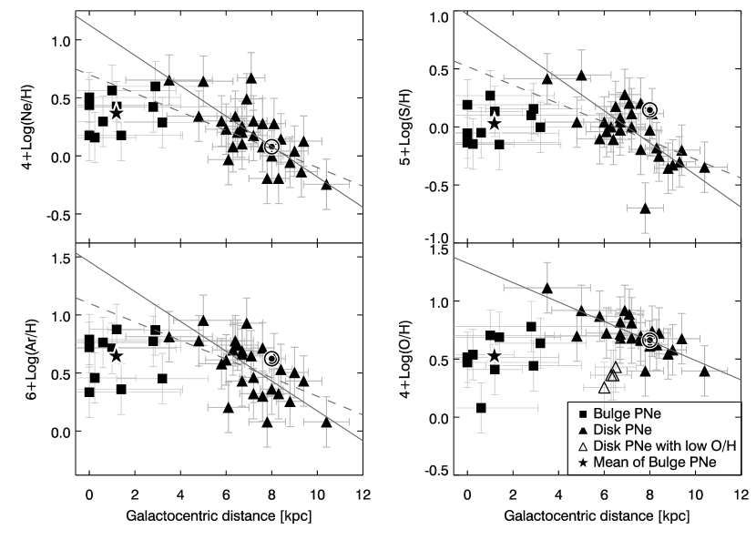
Figure 4.— The argon, neon, sulfur, and oxygen abundances of GBPNe and GDPNe versus the galactocentric distance. GBPNe are represented by filled squares and GDPNe by filled triangles while the assumed solar metallicity as discussed in Pottasch & Bernard-Salas (2006) is represented by the sun symbol, and the star indicates the mean of the GBPNe abundances. The solid grey lines represent least squares fits to the GDPNe abundances, excluding from the fit to the oxygen abundance the four GDPNe that are thought to have depleted oxygen (as discussed in Pottasch & Bernard-Salas (2006); open triangles). The dashed grey lines in the plots of argon, neon, and sulfur represent the oxygen abundance slope passing through the solid line fit at 8 kpc. Coefficients of the linear fits to both GBPNe and GDPNe are given in Table 13. The GBPNe placed on the graph exactly at R_GC=0.0 kpc have unknown galactocentric distances and are not included when we perform a linear fit to the data. The y-axis range for all the plots spans 2.0 dex, so that equal slopes will look equal in the plots. Distance uncertainties are propagated from the statistical distance uncertainties while abundance uncertainties are assumed to be 50%.

Table 13Parameters of linear fits to abundance gradients in GBPNe and GDPNe.

Element	GBPNe		GDPNe
	y-int (dex)	slope (dex/kpc)	y-int (dex)	slope (dex/kpc)
neon	0.0 $\pm$ 0.9	0.2 $\pm$ 0.3	1.1 $\pm$ 0.3	-0.13 $\pm$ 0.04
sulfur	-0.2 $\pm$ 0.6	0.2 $\pm$ 0.3	1.0 $\pm$ 0.3	-0.14 $\pm$ 0.04
argon	-12  $\pm$ 13	8   $\pm$ 260	1.5 $\pm$ 0.3	-0.13 $\pm$ 0.04
oxygen	-0.0 $\pm$ 0.9	0.3 $\pm$ 0.6	1.3 $\pm$ 0.3	-0.08 $\pm$ 0.03

5.2. Crystalline Silicates

Prior to ISO, crystalline silicates had only been observed in solar system comets (e.g. Hanner et al., 1994) and in $\beta$ Pic, a debris disk system (Knacke et al., 1993). ISO and now Spitzer have observed crystalline silicates in many sources. However, it is remarkable that we observe crystalline silicates in every single one of the GBPNe. We suggest here that this is because the GBPNe have disks.

In their ISO study of crystalline silicate dust around evolved stars, Molster (2000) and Molster et al. (2002) make mean continuum subtracted spectra for sources which are thought to have a dusty disk (disk sources) and sources which are expected to have a normal outflow (outflow sources). They find that the dust features of disk and outflow sources show definitive differences in strength, shape, and position of their dust features. In Figure 5 we plot normalized mean spectra of our GBPNe for the 28 and 33 µm features and compare them to the normalized mean disk and outflow spectra from Molster et al. (2002). Both the 28 and 33 µm complexes in our GBPNe look similar to the mean disk sources in Molster et al. (2002), but Molster et al. (2002) have several cautions about their mean spectra (for example, the ISO SWS band 3E, which covers the $\sim$27.5–29.2 µm, is known to have less reliable calibration). However, the similarity of the crystalline silicate dust features in our GBPNe to those of Molster’s disk sources gives indirect evidence that the silicates in our GBPNe are in disks.

If the crystalline silicates in these GBPNe are in fact in disks, then they point toward binary evolution of the progenitor stars. Edgar et al. (2007) ran numerical models that show how a binary companion can shape the AGB wind to form a crystalline dust torus. In their models, the shock temperatures reached when the wind blows past the companion anneal the dust and make it crystalline. They conclude that “Crystalline dust torii provide strong evidence for binary interactions in AGB winds.” As we discuss later in §5.4, over half of the GBPNe in this study show dual chemistry, which also implies binary evolution.

In our GBPNe sample, all of the nebulae show crystalline silicates, indicative of oxygen-rich material. Previous studies have found a low C/O ratio in GBPNe compared to GDPNe (e.g. Walton et al., 1993; Wang & Liu, 2007; Casassus et al., 2001). The higher fraction of O-rich PNe in the Bulge compared to the Disk implies that the Bulge should have a larger injection of silicate grains into its interstellar medium (ISM) than the Disk (Casassus et al., 2001).

Figure 5.— Normalized and shifted mean 28 and 33 µm spectra of our GBPNe compared to the mean disk and outflow sources from Molster et al. (2002).

5.3. PAHs

PAHs can be separated into different classes based on the position of their 6.2 µm and 7.7 µm peaks. Class A PAHs peak at shorter wavelengths than class B, which peak at shorter wavelengths than class C (Peeters et al., 2002). Figure 3 shows the peak positions for the different classes of PAHs along with the GBPNe PAH features. The GBPNe in this study have class A, AB, and B PAHs, and thus have PAH profiles similar to GDPNe. The lack of type C PAHs in the PNe indicates that their PAHs are all processed, i.e. the aliphatic component is negligible (Sloan et al., 2007).

The PAH flux ratios F_7.7µm/F_11.2µm and F_6.2µm/F_11.2µm both trace the ionization fraction of the PAHs, and are often plotted against each other in a figure. The GBPNe studied here have F_7.7µm/F_11.2µm between 1 and 3, and F_6.2µm/F_11.2µm between 0.5 and 1.4, and follow the same trend as Galactic Disk and Magellanic Cloud PNe (Bernard-Salas et al., in preparation).

5.4. Dual Chemistry Nebulae

ISO detected crystalline silicates and PAHs simultaneously in [WR] PNe — those PNe with H-poor and C-rich WR-type central stars (Waters et al., 1998). This dual chemistry is unusual in GDPNe (Bernard-Salas & Tielens, 2005). However, in our sample of GBPNe, six of the eleven nebulae have dual chemistry, showing both crystalline silicates and PAHs in their spectra. The fraction of [WR] PNe is significantly larger in the Bulge than the Disk (Górny et al., 2004), and thus the large fraction of PNe in the Bulge exhibiting dual chemistry makes sense. Possible explanations for this dual chemistry include (Little-Marenin, 1986; Willems & de Jong, 1986; Waters et al., 1998; Cohen et al., 1999): (1) a thermal pulse recently ($\lesssim$ 1000 years ago) turned an O-rich outflow into a C-rich one, and (2) the central star of the PN is in a binary system and the silicate grains orbit the system in a disk that existed long before the PN.

What explains how the majority of our GBPNe show dual chemistry? The explanation of a thermal pulse at the end of the AGB having suddenly changed the chemical composition of the central star from O-rich to C-rich within the last thousand years seems implausible because it is unlikely that we would catch so many GBPNe in this short stage (e.g. Lloyd Evans, 1991). A growing body of evidence supports the binary system with an old silicate disk explanation of dual chemistry in PNe and late-type stars (Waters et al., 1998; Molster et al., 2001; Matsuura et al., 2004). Taking one of these studies as an example, Matsuura et al. (2004) present mid-IR images of the post-AGB star IRAS 16279-4757 which shows both PAHs and crystalline silicates. Their images and model of this star imply that it has a C-rich bipolar outflow with an inner low-density C-rich region surrounded by an outer dense O-rich torus, indicating that mixed chemistry and morphology are related; mixed chemistry may point to binary evolution.

Other evidence also suggests that many of our GBPNe probably have binaries with silicate disks: (1) $\sim$40% of compact PNe in the Bulge have binary-induced morphologies (Zijlstra, 2007); (2) binary-induced novae are observed to be concentrated in the bulge of the galaxy M31 (e.g. Shafter & Irby, 2001; Rosino, 1973), and thus perhaps in the Bulge of our galaxy as well; (3) asymmetric (e.g. bipolar, quadrupolar) morphology is more common in PNe in high metallicity environments than in low metallicity ones (Stanghellini et al., 2003); (4) the current study showing the similarity of the mean GBPNe spectra to the mean disk spectra of Molster et al. 2002 (§5.2); and (5) the silicates are crystalline and not amorphous, indicating that they have been blasted over time and are likely stored in a disk (Molster et al., 1999). Thus it seems likely that the GBPNe in our sample with dual chemistry have a binary at their center with a silicate disk that formed long before the PN stage, while the PAHs reside in the PN outflow itself, possibly shooting out along the poles.

6. Conclusions

We extract the Spitzer IRS spectra of eleven PNe in the Bulge to study their abundances and dust properties. We conclude that:

(1) The abundances of argon, neon, sulfur, and oxygen are significantly lower in the PNe in the Bulge than the abundances for the Bulge predicted by the abundance gradient in the Disk, consistent with the idea that the Bulge and Disk evolved separately.

(2) All of the spectra in our sample of PNe in the Bulge show crystalline silicates, indicating that these crystalline silicates are likely stored in disks, which would further imply that the progenitor stars of these PNe evolved in binary systems.

(3) Six of the eleven spectra of PNe in the Bulge in our sample show PAHs in addition to the crystalline silicates. This dual chemistry also points toward binary evolution: the PAHs are in the current PN outflow and the crystalline silicates reside in a old disk created by binary interaction.

References

- Acker et al. (1992) Acker, A., Marcout, J., Ochsenbein, F., Stenholm, B., & Tylenda, R. 1992, Strasbourg - ESO catalogue of galactic planetary nebulae. Part 1; Part 2 (Garching: European Southern Observatory, 1992)
- Acker et al. (1991) Acker, A., Raytchev, B., Koeppen, J., & Stenholm, B. 1991, A&AS, 89, 237
- Allamandola et al. (1989) Allamandola, L. J., Tielens, G. G. M., & Barker, J. R. 1989, ApJS, 71, 733
- Beaulieu et al. (1999) Beaulieu, S. F., Dopita, M. A., & Freeman, K. C. 1999, ApJ, 515, 610
- Bensby & Lundström (2001) Bensby, T. & Lundström, I. 2001, A&A, 374, 599
- Bernard-Salas et al. (2008) Bernard-Salas, J., Pottasch, S. R., Gutenkunst, S., Morris, P. W., & Houck, J. R. 2008, ApJ, 672, 274
- Bernard-Salas & Tielens (2005) Bernard-Salas, J. & Tielens, A. G. G. M. 2005, A&A, 431, 523
- Cahn et al. (1992) Cahn, J. H., Kaler, J. B., & Stanghellini, L. 1992, A&AS, 94, 399
- Casassus et al. (2001) Casassus, S., Roche, P. F., Aitken, D. K., & Smith, C. H. 2001, MNRAS, 327, 744
- Ciardullo et al. (1999) Ciardullo, R., Bond, H. E., Sipior, M. S., Fullton, L. K., Zhang, C.-Y., & Schaefer, K. G. 1999, AJ, 118, 488
- Clegg et al. (1987) Clegg, R. E. S., Harrington, J. P., Barlow, M. J., & Walsh, J. R. 1987, ApJ, 314, 551
- Cohen et al. (1999) Cohen, M., Barlow, M. J., Sylvester, R. J., Liu, X.-W., Cox, P., Lim, T., Schmitt, B., & Speck, A. K. 1999, ApJ, 513, L135
- Condon & Kaplan (1998) Condon, J. J. & Kaplan, D. L. 1998, ApJS, 117, 361
- Cuisinier et al. (2000) Cuisinier, F., Maciel, W. J., Köppen, J., Acker, A., & Stenholm, B. 2000, A&A, 353, 543
- Cunha & Smith (2006) Cunha, K. & Smith, V. V. 2006, ApJ, 651, 491
- Durand et al. (1998) Durand, S., Acker, A., & Zijlstra, A. 1998, A&AS, 132, 13
- Edgar et al. (2007) Edgar, R. G., Nordhaus, J., Blackman, E., & Frank, A. 2007, ArXiv e-prints, 709
- Eisenhauer et al. (2005) Eisenhauer, F., et al. 2005, ApJ, 628, 246
- Escudero et al. (2004) Escudero, A. V., Costa, R. D. D., & Maciel, W. J. 2004, A&A, 414, 211
- Exter et al. (2004) Exter, K. M., Barlow, M. J., & Walton, N. A. 2004, MNRAS, 349, 1291
- Ferreras et al. (2003) Ferreras, I., Wyse, R. F. G., & Silk, J. 2003, MNRAS, 345, 1381
- Fluks et al. (1994) Fluks, M. A., Plez, B., The, P. S., de Winter, D., Westerlund, B. E., & Steenman, H. C. 1994, A&AS, 105, 311
- Fulbright et al. (2007) Fulbright, J. P., McWilliam, A., & Rich, R. M. 2007, ApJ, 661, 1152
- Górny et al. (2004) Górny, S. K., Stasińska, G., Escudero, A. V., & Costa, R. D. D. 2004, A&A, 427, 231
- Groenewegen et al. (2008) Groenewegen, M. A. T., Udalski, A., & Bono, G. 2008, ArXiv e-prints, 801
- Guiles et al. (2007) Guiles, S., Bernard-Salas, J., Pottasch, S. R., & Roellig, T. L. 2007, ApJ, 660, 1282
- Hanner et al. (1994) Hanner, M. S., Lynch, D. K., & Russell, R. W. 1994, ApJ, 425, 274
- Helou & Walker (1988) Helou, G. & Walker, D. W., eds. 1988, Infrared astronomical satellite (IRAS) catalogs and atlases. Volume 7: The small scale structure catalog, Vol. 7
- Higdon et al. (2004) Higdon, S. J. U., et al. 2004, PASP, 116, 975
- Houck et al. (2004) Houck, J. R., et al. 2004, ApJS, 154, 18
- Hummer & Storey (1987) Hummer, D. G. & Storey, P. J. 1987, MNRAS, 224, 801
- Karakas (2003) Karakas, A. I. 2003, Asymptotic Giant Branch Stars: their influence on binary systems and the interstellar medium (Thesis, Monash Univ. Melbourne. Available at http://www.mso.anu.edu.au/ akarakas/research.html)
- Karakas & Lattanzio (2003) Karakas, A. I. & Lattanzio, J. C. 2003, Publications of the Astronomical Society of Australia, 20, 393
- Knacke et al. (1993) Knacke, R. F., Fajardo-Acosta, S. B., Telesco, C. M., Hackwell, J. A., Lynch, D. K., & Russell, R. W. 1993, ApJ, 418, 440
- Lecureur et al. (2007) Lecureur, A., Hill, V., Zoccali, M., Barbuy, B., Gómez, A., Minniti, D., Ortolani, S., & Renzini, A. 2007, A&A, 465, 799
- Little-Marenin (1986) Little-Marenin, I. R. 1986, ApJ, 307, L15
- Lloyd Evans (1991) Lloyd Evans, T. 1991, MNRAS, 249, 409
- López-Corredoira et al. (2000) López-Corredoira, M., Hammersley, P. L., Garzón, F., Simonneau, E., & Mahoney, T. J. 2000, MNRAS, 313, 392
- Martín-Hernández et al. (2002) Martín-Hernández, N. L., et al. 2002, A&A, 381, 606
- Matsuura et al. (2004) Matsuura, M., et al. 2004, ApJ, 604, 791
- Minniti et al. (1995) Minniti, D., Olszewski, E. W., Liebert, J., White, S. D. M., Hill, J. M., & Irwin, M. J. 1995, MNRAS, 277, 1293
- Molster (2000) Molster, F. J. 2000, PhD thesis, FNWI: Sterrenkundig Instituut Anton Pannekoek, Postbus 19268, 1000 GG Amsterdam, The Netherlands
- Molster et al. (2002) Molster, F. J., Waters, L. B. F. M., & Tielens, A. G. G. M. 2002, A&A, 382, 222
- Molster et al. (2001) Molster, F. J., Yamamura, I., Waters, L. B. F., Nyman, L.-Å., Käufl, H.-U., de Jong, T., & Loup, C. 2001, A&A, 366, 923
- Molster et al. (1999) Molster, F. J., et al. 1999, Nature, 401, 563
- Peeters et al. (2002) Peeters, E., Hony, S., Van Kerckhoven, C., Tielens, A. G. G. M., Allamandola, L. J., Hudgins, D. M., & Bauschlicher, C. W. 2002, A&A, 390, 1089
- Pottasch (1984) Pottasch, S. R., ed. 1984, Planetary nebulae - A study of late stages of stellar evolution
- Pottasch & Beintema (1999) Pottasch, S. R. & Beintema, D. A. 1999, A&A, 347, 975
- Pottasch & Bernard-Salas (2006) Pottasch, S. R. & Bernard-Salas, J. 2006, A&A, 457, 189
- Pottasch et al. (2007) Pottasch, S. R., Bernard-Salas, J., & Roellig, T. L. 2007, A&A, 471, 865
- Ratag et al. (1997) Ratag, M. A., Pottasch, S. R., Dennefeld, M., & Menzies, J. 1997, A&AS, 126, 297
- Ratag et al. (1992) Ratag, M. A., Pottasch, S. R., Dennefeld, M., & Menzies, J. W. 1992, A&A, 255, 255
- Reid (1993) Reid, M. J. 1993, ARA&A, 31, 345
- Rolleston et al. (2000) Rolleston, W. R. J., Smartt, S. J., Dufton, P. L., & Ryans, R. S. I. 2000, A&A, 363, 537
- Rosino (1973) Rosino, L. 1973, A&AS, 9, 347
- Rubin et al. (1988) Rubin, R. H., Simpson, J. P., Erickson, E. F., & Haas, M. R. 1988, ApJ, 327, 377
- Ruffle et al. (2004) Ruffle, P. M. E., Zijlstra, A. A., Walsh, J. R., Gray, M. D., Gesicki, K., Minniti, D., & Comeron, F. 2004, MNRAS, 353, 796
- Schutte et al. (1993) Schutte, W. A., Tielens, A. G. G. M., & Allamandola, L. J. 1993, ApJ, 415, 397
- Shafter & Irby (2001) Shafter, A. W. & Irby, B. K. 2001, ApJ, 563, 749
- Shaver et al. (1983) Shaver, P. A., McGee, R. X., Newton, L. M., Danks, A. C., & Pottasch, S. R. 1983, MNRAS, 204, 53
- Simpson et al. (1995) Simpson, J. P., Colgan, S. W. J., Rubin, R. H., Erickson, E. F., & Haas, M. R. 1995, ApJ, 444, 721
- Sloan et al. (2007) Sloan, G. C., et al. 2007, ApJ, 664, 1144
- Stanghellini et al. (2003) Stanghellini, L., Shaw, R. A., Balick, B., Mutchler, M., Blades, J. C., & Villaver, E. 2003, ApJ, 596, 997
- Tylenda et al. (1992) Tylenda, R., Acker, A., Stenholm, B., & Koeppen, J. 1992, A&AS, 95, 337
- van de Steene & Zijlstra (1995) van de Steene, G. C. & Zijlstra, A. A. 1995, A&A, 293, 541
- Walton et al. (1993) Walton, N. A., Barlow, M. J., & Clegg, R. E. S. 1993, in IAU Symposium, Vol. 153, Galactic Bulges, ed. H. Dejonghe & H. J. Habing, 337–+
- Wang & Liu (2007) Wang, W. & Liu, X. . 2007, ArXiv e-prints, 707
- Waters et al. (1998) Waters, L. B. F. M., et al. 1998, A&A, 331, L61
- Werner et al. (2004) Werner, M. W., et al. 2004, ApJS, 154, 1
- Willems & de Jong (1986) Willems, F. J. & de Jong, T. 1986, ApJ, 309, L39
- Zhang (1995) Zhang, C. Y. 1995, ApJS, 98, 659
- Zijlstra (2007) Zijlstra, A. A. 2007, Baltic Astronomy, 16, 79