On the algebraic geometry of polynomial dynamical systems

Abstract.

This paper focuses on polynomial dynamical systems over finite fields. These systems appear in a variety of contexts, in computer science, engineering, and computational biology, for instance as models of intracellular biochemical networks. It is shown that several problems relating to their structure and dynamics, as well as control theory, can be formulated and solved in the language of algebraic geometry.

1. Introduction

The study of the dynamics of polynomial maps as time-discrete dynamical systems has a long tradition, in particular polynomials over the complex numbers leading to fractal structures. An example of more recent work using techniques from algebraic geometry includes the study of the algebraic and topological entropy of iterates of monomial mappings $f=(f_{1},\ldots,f_{n})$ over subsets of $\mathbf{C}^{n}$ hasselblatt:07 . The study of iterates of polynomial mappings (or, more generally, rational maps) over the $p$-adic numbers originally arose in Diophantine geometry Call:93 . For more recent work see, e.g., vivaldi:2001 . Finally, there is a long tradition of studying the iterates of polynomial maps $f:\mathbf{F}_{q}\longrightarrow\mathbf{F}_{q}$ over finite fields, primarily using techniques from combinatorics and algebraic number theory (see, e.g., LM1 ; LM2 .

The general case of finite dynamical systems

$$f=(f_{1},\ldots,f_{n}):\mathbf{F}_{q}^{n}\longrightarrow\mathbf{F}_{q}^{n},$$

with $f_{i}\in\mathbf{F}_{q}[x_{1},\ldots,x_{n}]$ has long been of interest in the special case $q=2$, which includes Boolean networks and cellular automata. They are of considerable interest in engineering and computer science, for instance. Since the 1960s they are also being used increasingly as models of diverse biological and social networks.

The underlying mathematical questions in these studies for different fields are similar. They relate primarily to understanding the long-term behavior of the iterates of the mapping. In the case of monomial mappings, the matrix of exponents is usually the right mathematical object to analyze by using different methods based on the ground field. Generally, one would like to be able to use some feature of the structure of the coordinate functions $f_{i}$ to deduce properties of the structure of the phase space of the system $f$ which represents the system’s dynamics. For finite systems, i.e., polynomial dynamical systems $f$ over a finite field $k$, the phase space $\mathcal{P}(f)$ has the form of a directed graph with vertices the elements of $k^{n}$. There is an edge $\mathbf{v}\longrightarrow\mathbf{w}$ in $\mathcal{P}(f)$ if $f(\mathbf{v})=\mathbf{w}$. Since the graph has finitely many vertices it is easy to see that each component has the structure of a directed limit cycle, with trees (transients) feeding into each of the nodes in the cycle.

Example 1.1.

Let $f:\mathbf{F}_{3}^{2}\longrightarrow\mathbf{F}_{3}^{2}$ be given by $f(x_{1},x_{2})=(1-x_{1}x_{2},1+2x_{2})$. The phase space of $f$ has two components, containing two limit cycles: one of length two and one of length three. See Figure 1 (right). The dependency relations among the variables are encoded in the dependency graph in Figure 1 (left).

    

Figure 1. The dependency graph (left) and the phase space $\mathcal{P}(f)$ (right) of the finite dynamical system in Example 1.1.

In this case the information of interest is the number of components, the length of the limit cycles, and, possibly, the structure of the transient trees. It is also of interest to study the sequence of iterates $f^{r}$ of $f$.

In recent years interest in polynomial dynamical systems over general finite fields has arisen also because they are useful as multistate generalizations of Boolean network models for biochemical networks, such as gene regulatory networks. In particular, the problem of network inference from experimental data can be formulated and solved in this framework. The tools used are very similar to those developed for the solution of problems in the statistical field of design of experiments and which led directly to the new field of algebraic statistics. (This connection is made explicit in LS:des_exp .) Analyzing finite dynamical systems models of molecular networks requires tools that provide information about network dynamics from information about the system. Since the systems arising in applications can be quite high-dimensional it is not feasible to carry out such an analysis by exhaustive enumeration of the phase space. Thus, the studies of polynomial dynamics mentioned earlier become relevant to this type of application. Finally, an important role of models in biology and engineering is their use for the construction of controllers, be it for drug delivery to fight cancer or control of an airfoil. Here too, approaches have been developed for control systems in the context of polynomial dynamical systems.

Here we describe this circle of ideas and some existing results. Along the way we will mention open problems that arise. We believe that algebraic geometry can play an essential role as a conceptual and computational tool in this application area. Consistent with our specific research interests we will restrict ourselves to polynomial dynamical systems over finite fields.

2. Finite dynamical systems

Let $k$ be a finite field and let

$$f=(f_{1},\ldots,f_{n}):k^{n}\longrightarrow k^{n}$$

be a mapping. It is well-known that the coordinate functions $f_{i}$ can be represented as polynomials [LN, , p. 369], and this representation is unique if we require that the degree of every variable in every term of the $f_{i}$ is less than $|k|$. If $k$ is the field with two elements, then it is easily seen that $f$ represents a Boolean network. Conversely, every Boolean network can be represented in polynomial form. Hence, polynomial dynamical systems over a finite field, which we shall call finite dynamical systems include all time-discrete dynamical systems over finite fields. Iteration of $f$ generates dynamics which is captured by the phase space $\mathcal{P}(f)$ of $f$, defined above. We will first focus on the problem of inferring information about the structure of $\mathcal{P}(f)$ from the polynomials $f_{i}$.

In principle, a lot of information about $\mathcal{P}(f)$ can be gained by solving systems of polynomial equations. For instance, the fixed points of $f$ are precisely the points on the variety given by the system

$$f_{1}(x_{1},\ldots,x_{n})-x_{1}=0,\ldots,f_{n}(x_{1},\ldots,x_{n})-x_{n}=0.$$

The points of period 2 are the points on the variety given by the system $f_{i}^{2}(x_{1},\ldots,x_{n})-x_{i}=0,i=1,\ldots,n$, and so on. But often the most efficient way of solving these systems over a finite field, in particular a small finite field, is by exhaustive enumeration, which is not feasible for large $n$. A more modest goal would be to find out the number of periodic points of a given period, that is, the number of points on the corresponding variety. For finite fields this is also quite difficult without the availability of good general tools, and much work remains to be done in this direction.

The case of linear systems is the only case that has so far been treated systematically, using methods from linear algebra, as one might expect. Let $M$ be the matrix of $f$. Then complete information about the number of components in $\mathcal{P}(f)$, the lengths of all the limit cycles and the structure of the transient trees can be computed from the invariant factors of $A$, together with the orders of their irreducible factors He . See JLSV for an implementation of this algorithm in the computer algebra system Singular Sing .

There are results available for several other special families of systems, using ad hoc combinatorial and graph-theoretical methods. For instance, we have investigated the case where all the $f_{i}$ are monomials. It is of interest to characterize monomial systems all of whose periodic points are fixed points. For the field with two elements this characterization can be given in terms of the dependency graph of the system. This graph has as vertices the variables $x_{1},\ldots,x_{n}$. There is a directed edge $x_{i}\rightarrow x_{j}$ if $x_{i}$ appears in $f_{j}$; see Figure 1(left) for an example. Given a directed graph it can be decomposed into strongly connected components, with each component a subgraph in which each vertex can be reached from every other vertex by a directed path. Associated to a strongly connected graph we have its loop number which is defined as the greatest common divisor of the lengths of all directed loops in the graph based at a fixed vertex. (It is easy to see that this number is independent of the vertex chosen.) The loop number is also known as the index of imprimitivity of the graph.

It is shown in colon:04 that the length of any cycle in the phase space of a monomial system $f$ must divide the loop number of its dependency graph. In particular, we have the following result about fixed-point monomial systems.

Theorem 2.1 (colon:04 ).

All periodic points of a monomial system $f$ are fixed points if and only if each strongly connected component of the dependency graph of $f$ has loop number 1.

The study of monomial systems over general finite fields can be reduced to studying linear and Boolean systems CJLS . There are other interesting families of systems whose dynamics has been studied. One such family is that of Boolean networks constructed from nested canalyzing functions. These were introduced and studied in kpst03 ; kauffman:04 . The context is the use of Boolean networks as models for gene regulatory networks initiated by S. Kauffman Kauffman:69 . We first recall the definitions of canalyzing and nested canalyzing functions from kpst03 .

Definition 2.2.

A canalyzing function is a Boolean function with the property that one of its inputs alone can determine the output value, for either “true” or “false” input. This input value is referred to as the canalyzing value, while the output value is the canalyzed value.

Example 2.3.

The function $f(x,y)=xy$ is a canalyzing function in the variable $x$ with canalyzing value 0 and canalyzed value 0. However, the function $f(x,y)=x+y$ is not canalyzing in either variable.

Nested canalyzing functions are a natural specialization of canalyzing functions. They arise from the question of what happens when the function does not get the canalyzing value as input but instead has to rely on its other inputs. Throughout this paper, when we refer to a function of $n$ variables, we mean that $f$ depends on all $n$ variables. That is, for $1\leq i\leq n$, there exists $(a_{1},\dots,a_{n})\in\mathbf{F}_{2}^{n}$ such that $f(a_{1},\dots,a_{i-1},a_{i},a_{i+1},\dots,a_{n})\neq f(a_{1},\dots,a_{i-1},1+a_{i},a_{i+1},\dots,a_{n})$.

Definition 2.4.

A Boolean function $f$ in $n$ variables is a nested canalyzing function(NCF) in the variable order $x_{1},x_{2},\ldots,x_{n}$ with canalyzing input values $a_{1},\dots,a_{n}$ and canalyzed output values $b_{1},\dots,b_{n}$, respectively, if it can be expressed in the form

$$f(x_{1},x_{2},\ldots,x_{n})=\begin{cases}b_{1}&~{}{\rm if}~{}x_{1}=a_{1},\\ b_{2}&~{}{\rm if}~{}x_{1}\neq a_{1}~{}{\rm and}~{}x_{2}=a_{2},\\ b_{3}&~{}{\rm if}~{}x_{1}\neq a_{1}~{}{\rm and}~{}x_{2}\neq a_{2}~{}{\rm and}~{}x_{3}=a_{3},\\ \vdots&\hskip 28.45274pt\vdots\\ b_{n}&~{}{\rm if}~{}x_{1}\neq a_{1}~{}{\rm and}~{}\cdots~{}{\rm and}~{}x_{n-1}\neq a_{n-1}~{}{\rm and}~{}x_{n}=a_{n},\\ b_{n}+1&~{}{\rm if}~{}x_{1}\neq a_{1}~{}{\rm and}~{}\cdots~{}{\rm and}~{}x_{n}\neq a_{n}.\end{cases}$$

Example 2.5.

The function $f(x,y,z)=x(y-1)z$ is nested canalyzing in the variable order $x,y,z$ with canalyzing values 0,1,0 and canalyzed values 0,0,0, respectively. However, the function $f(x,y,z,w)=xy(z+w)$ is not a nested canalyzing function because if $x\neq 0$ and $y\neq 0$, then the value of the function is not constant for any input values for either $z$ or $w$.

It is shown in kauffman:04 through extensive computer simulations that Boolean networks constructed from nested canalyzing functions show very stable dynamic behavior, with short transient trees and a small number of components in their phase space. It is this type of dynamics that gene regulatory networks are thought to exhibit. It is thus reasonable to use this class of functions preferentially in modeling such networks. To do so effectively it is necessary to have a better understanding of the properties of this class, for instance, how many nested canalyzing functions with a given number of variables there are.

In JLR a parametrization of this class is given as follows. The first step is to view Boolean functions as polynomials using the following translation:

$$x\wedge y=x\cdot y,\,x\vee y=x+y+xy,\,\neg x=x+1.$$

It is shown in JLR that the ring of Boolean functions is isomorphic to the quotient ring $R=\mathbf{F}_{2}[x_{1},\dots,x_{n}]/I$, where $I=\langle x_{i}^{2}-x_{i}:1\leq i\leq n\rangle$. Indexing monomials by the subsets of $[n]:=\{1,\ldots,n\}$ corresponding to the variables appearing in the monomial, we can write the elements of $R$ as

$$R=\{\displaystyle\sum_{S\subseteq[n]}c_{S}\prod_{i\in S}x_{i}\,:\,c_{S}\in\mathbf{F}_{2}\}.$$

As a vector space over $\mathbf{F}_{2}$, $R$ is isomorphic to $\mathbf{F}_{2}^{2^{n}}$ via the correspondence

$$R\ni\displaystyle\sum_{S\subseteq[n]}c_{S}\prod_{i\in S}x_{i}\longleftrightarrow(c_{\emptyset},\dots,c_{[n]})\in\mathbf{F}_{2}^{2^{n}},$$

for a given fixed total ordering of all square-free monomials. That is, a polynomial function corresponds to the vector of coefficients of the monomial summands. The main result in JLR is the identification of the set of nested canalyzing functions in $R$ with a subset $V^{ncf}$ of $\mathbf{F}_{2}^{2^{n}}$ by imposing relations on the coordinates of its elements.

Definition 2.6.

Let $\sigma$ be a permutation of the elements of the set $[n]$. We define a new order relation $<_{\sigma}$ on the elements of $[n]$ as follows: $\sigma(i)<_{\sigma}\sigma(j)$ if and only if $i<j$. Let $r_{S}^{\sigma}$ be the maximum element of a nonempty subset $S$ of $[n]$ with respect to the order relation $<_{\sigma}$. For any nonempty subset $S$ of $[n]$, the completion of S with respect to the permutation $\sigma$, denoted by $[r_{S}^{\sigma}]$, is the set $[r_{S}^{\sigma}]=\{\sigma(1),\sigma(2),\ldots,\sigma(r_{S})\}$.

Note that, if $\sigma$ is the identity permutation, then the completion is $[r_{S}]$ := $\{1,2,\ldots,r_{S}\}$, where $r_{S}$ is the largest element of $S$.

Theorem 2.7.

[AB2007, , Thm. 1] Let $f\in R$ and let $\sigma$ be a permutation of the set $[n]$. The polynomial $f$ is a nested canalyzing function in the order $x_{\sigma(1)},x_{\sigma(2)},\ldots,x_{\sigma(n)}$, with input values $a_{\sigma(i)}$ and corresponding output values $b_{\sigma(i)},1\leq i\leq n$, if and only if $c_{[n]}=1$ and, for any proper subset $S\subseteq[n]$,

$$c_{S}=c_{[r_{S}^{\sigma}]}\prod_{\sigma(i)\in[r_{S}^{\sigma}]\backslash S}c_{[n]\backslash\{\sigma(i)\}}.$$

Corollary 2.8.

[AB2007, , Cor. 1] The set of points in $\mathbf{F}_{2}^{2^{n}}$ corresponding to nested canalyzing functions in the variable order $x_{\sigma(1)},x_{\sigma(2)},\ldots,x_{\sigma(n)}$, denoted by $V_{\sigma}^{ncf}$, is defined by

$$V_{\sigma}^{ncf}=\{(c_{\emptyset},\dots,c_{[n]})\in\mathbf{F}_{2}^{2^{n}}:c_{[n]}=1,\,c_{S}=c_{[r_{S}^{\sigma}]}\prod_{\sigma(i)\in[r_{S}^{\sigma}]\backslash S}c_{[n]\backslash\{\sigma(i)\}}\mbox{, for }S\subseteq[n]\}.$$

It was also shown in JLR that

$$V^{ncf} = \bigcup_{\sigma}V_{\sigma}^{ncf}.$$

Counting the points on this variety for small values of $n$ resulted in an integer sequence, which, with the help of the On-Line Encyclopedia of Integer Sequences (http://www.research.att.com/ njas/sequences/) led to the realization that the class of nested canalyzing functions is identical to the class of unate cascade functions that has been studied extensively in computer engineering literature. In particular, using this equality, one obtains a recursive formula for the number of nested canalyzing functions, see [JLR, , Corollary 2.11].

It is shown in AB2007 that the sets $V_{\sigma}^{ncf}$ are the irreducible components of $V^{ncf}$. Precisely, it is shown that for all permutations $\sigma$ on $[n]$, the ideal of the variety $V_{\sigma}^{ncf}$, denoted by $I_{\sigma}:=\mathds{I}(V_{\sigma}^{ncf})$, is a binomial prime ideal in the polynomial ring $\overline{\mathbf{F}}_{2}[\{c_{S}:S\subseteq[n]\}]$, where $\overline{\mathbf{F}}_{2}$ is the algebraic closure of $\mathbf{F}_{2}$.

It remains to study this toric variety in more detail. In particular, a generalization of the concept of nested canalyzing function to larger finite fields remains to be worked out. Also, the approach taken here can be applied to other classes of functions important in network modeling, such as threshold functions or monotone functions.

3. Network inference

Our motivation for much of the research described in the previous section comes from our work on one of the central problems in computational systems biology. Due to the availability of so-called ”omics” data sets it is now feasible to think about making large-scale mathematical models of molecular networks involving many gene transcripts (genomics), proteins (proteomics), and metabolites (metabolomics). One possible approach to this problem is to build a phenomenological model based solely or largely on the experimental data which can subsequently be refined with additional biological information about the mechanisms of interaction of the different molecular species. That is, given a data set, we are to infer a “most likely” mathematical or statistical model of the network that generated this data set. The biggest challenge is that typically the network that generated the data is high-dimensional (hundreds or thousands of molecular species/variables) and the available data sets are typically very small (tens or hundreds of data points). Also, general properties of such networks are not well-understood so that there are few general selection criteria. Therefore, it is not feasible to apply many of the existing network inference methods. In this context, two pieces of information about a molecular network are of interest to a life scientist: the “wiring diagram” of the network indicating which variables causally affect which others, and the long-term dynamic behavior of the network. Some network inference methods give only information about the wiring diagram, others provide both.

One possible modeling framework is that of polynomial dynamical systems over finite fields. In the 1960s, S. Kauffman proposed Boolean networks as good models for capturing key aspects of gene regulation Kauffman:69 . In the 1990s so-called logical models were proposed by R. Thomas Thomas:89 as models for biochemical network, which are multi-state time-discrete dynamical systems, with both deterministic and stochastic variants. In LS it was shown that the modeling framework of polynomial dynamical systems over finite fields is a good setting for the problem of network inference. As pointed out, these systems generalize Boolean networks and have many of the same features as logical models. The network inference problem can be formulated in this setting as follows.

Suppose that the biological system to be modeled contains $n$ variables, e.g., genes, and we measure $r+1$ time points $\mathbf{p}_{0},\ldots,\mathbf{p}_{r}$, using, e.g., gene chip technology, each of which can be viewed as an $n$-dimensional real-valued vector. The first step is to discretize the entries in the $\mathbf{p}_{i}$ into a prime number of states, which are viewed as entries in a finite field $k$. If we choose to discretize into two states by choosing a threshold, then we will obtain Boolean networks as models. The discretization step is crucial in this process as it represents the interface between the continuous and discrete worlds. Other network inference methods, such as most dynamic Bayesian network methods, also have to carry out this preprocessing step. Unfortunately, there is very little work that has been done on this problem. We have developed a new discretization method which is described in DVML . It compares favorably to other commonly used discretization methods, using different network inference methods.

Given this data set, an admissible model

$$f=(f_{1},f_{2},\ldots,f_{n}):k^{n}\longrightarrow k^{n}$$

consists of a dynamical system $f$ which satisfies the property that

$$f(\mathbf{p}_{j})=(f_{1}(\mathbf{p}_{j}),\ldots,f_{n}(\mathbf{p}_{j}))=\mathbf{p}_{j+1}.$$

The algorithm in LS then proceeds to select such a model $f$, which is the most likely one based on certain specified criteria. This is done by first reducing the problem to the case of one variable, that is, to the problem of selecting the $f_{i}$ separately. For this purpose, we compute the set of all functions $f_{i}$ such that $f_{i}(\mathbf{p}_{j})=\mathbf{p}_{j+1}^{i}$, that is, all polynomial functions $f_{i}$ whose value on $\mathbf{p}_{j}$ is the $i$th coordinate of $\mathbf{p}_{j+1}$. This set can be represented as the coset $f^{0}+I$, where $f^{0}$ is a particular such function and $I\subset k[x_{1},\ldots,x_{n}]$ is the ideal of all polynomials that vanish on the given data set, also known as the ideal of points of ${\mathbf{p}}_{1},\ldots,{\mathbf{p}}_{r-1}$. The algorithm then chooses the normal form of an interpolating polynomial $f^{0}$, based on a chosen term order. One drawback of the algorithm is that this choice of term order is typically random and can of course significantly affect the form of the model.

Modifications of the algorithm in LS have been constructed. The algorithm in JLSS starts with only data as input and computes all possible minimal wiring diagrams of polynomial models that fit the given data and outputs a most likely one, based on one of several possible model scoring methods. It does not depend on the choice of a term order. The algorithm is based on the observation that if $f_{i}$ is the $i$-th coordinate function of a model and $\mathbf{p},\mathbf{q}$ are data points such that $f_{i}(\mathbf{p})\neq f_{i}(\mathbf{q})$, then the function $f_{i}$ must involve at least some of the variables corresponding to coordinates in which $\mathbf{p}$ and $\mathbf{q}$ differ. This observation can be encoded in a monomial ideal $M$ which is generated by all monomials of the form

$$\prod_{\mathbf{p}_{j}\neq\mathbf{q}_{j}}x_{j}$$

for all pairs of points $\mathbf{p}\neq\mathbf{q}$ such that $f_{i}(\mathbf{p})\neq f_{i}(\mathbf{q})$. Now let $P=\langle x_{j_{1}},\ldots,x_{j_{t}}\rangle$ be a minimal prime of $M$. Then it is not hard to see that the generators of $P$ induce a minimal wiring diagram for $f_{i}$. Conversely, every such minimal diagram provides generators for a minimal prime of the ideal $M$. This algorithm has been implemented in Macaulay2 M2 . The algorithm comes with a collection of probability distributions on the set of minimal primes that can be used for model selection.

Another approach to the problem of dependency of the model selection process in LS on the chosen term order is taken in DJSL . The algorithm there uses the Gröbner fan of the ideal of points as a computational tool to find a most likely wiring diagram. It is clear that an upper bound for the number of different models one can obtain from the algorithm in LS by varying the choice of term order is given by the number of cones in the Gröbner fan. The algorithm in DJSL uses information about the frequency of appearance of the different variables in models built for each cone to build a consensus wiring diagram from this collection of possible models. It computes the Deegan-Packel index of power DP to rank variables in order of significance. This index was introduced in Fetrow , where it was computed using a Monte Carlo algorithm to generate random term orders. The use of the Gröbner fan allows a systematic computation of this index.

Note that the model space $f^{0}+I$ contains all possible polynomial functions that fit the given data. In order to improve the performance of model selection algorithms it would be very useful to be able to select certain subspaces of functions that have favorable properties as models of particular biological systems, thereby reducing the model space. For instance, one might consider imposing certain constraints on the structure of the polynomials or on the resulting dynamics. The desire to find such constraints is what motivated the investigations described in the previous section. In order to select a class of polynomials with prescribed dynamics one needs to be able to link polynomial structure to dynamics in an algorithmic way. Similarly, in order to limit model selection to special classes of polynomials, such as nested canalyzing functions in the Boolean case, one must be able to identify efficiently the set of such functions from the model space $f^{0}+I$. This problem remains open.

4. Control of finite dynamical systems

Control of biological systems is an important aspect of computational biology, ranging from the control of intracellular biochemical pathways to chemotherapy drug delivery and control of epidemiological processes. In order to apply mathematical control theory techniques it is necessary to work with a mathematical model of the system for which control theoretic tools exist. There is of course a very rich control-theoretic literature for systems of differential equations. However, the problem has also been considered in the context of polynomial dynamical systems over finite fields ML1 ; ML2 ; RS1 . We briefly describe the general setting.

The framework developed before needs to be slightly modified to accommodate variables representing control inputs at each state transitions as well as constraints on these inputs and on the set of allowable initial conditions.

Definition 4.1.

A controlled finite dynamical system is a function

$$F:k^{n}\times k^{m}\longrightarrow k^{n},$$

where the first set of variables $x_{1},\ldots,x_{n}$ represents the state variables, and the second set $u_{1},\ldots,u_{m}$ represents the control variables. Furthermore, we have a system of polynomial equations

$$Q_{i}(x_{1},\ldots,x_{n};u_{1},\ldots,u_{m})=0,\,i=1,\ldots,r,$$

which defines the variety of admissible control inputs, and another system

$$P_{j}(x_{1},\ldots,x_{n})=0,\,j=1,\ldots,s,$$

which defines the variety of admissible initial conditions of the system. Finally, we have another polynomial system

$$U_{a}(x_{1},\ldots,x_{n})=0,\,a=1,\ldots,t,$$

which defines the variety of admissible final states.

A typical optimal control problem is then stated as follows. Given a controlled system $F$ and an admissible initialization $(x_{1},\ldots,x_{n})$, find a sequence of control inputs which drive the system to an admissible final state, in such a way that a suitably defined cost function is minimized. There are several ad hoc strategies of finding an optimal controller but much theoretical work remains to be done in this context.

In JVDL an application of this approach to a virus competition problem was given, which we describe here in some detail in order to illustrate the definitions. In a Petri dish the center is infected with two different suitably chosen virus strains. It can be observed experimentally that, as the infection spreads to the rest of the dish a clear pattern of segmentation occurs between the two virus populations, rather than the expected mixing of the two strains. Through addition of one or the other type of virus over time the segmentation pattern can be influenced. For instance, it is possible to contain one virus strain by strategically inoculating cells in the Petri dish with the other strain. A possible application of this observation might be that one can contain the spread of a very harmful virus by the strategic introduction of another, less harmful virus strain. In this context it would be of interest to develop optimal strategies for introducing the second strain.

This problem was treated in JVDL by representing the spread of the two virus populations as a polynomial dynamical system over the Galois field $k=GF(4)$ as follows. The Petri dish is represented by 331 concentrically arranged hexagonal cells, each of which is a variable of the system. Each cell can take on 4 possible states, corresponding to being uninfected (White), infected by one of the two strains (Green or Red), or infected by both (Yellow). We begin with an arbitrary initialization of the center of the Petri dish, which is represented by the 19 innermost cells. That is, we make an arbitrary assignment of the 4 colors to these cells. All remaining cells are assigned White. The goal is to apply a series of control inputs as the infection spreads, which prevents the Red virus from spreading to the edge of the Petri dish. That is, a desirable final state of the system is any state for which the outermost ring of cells is infected only with Green virus. See Figure 2.

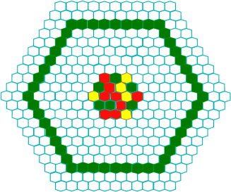
Figure 2. Control objective.

The rules governing the spread of infection are as follows:

1. If a cell has only one infected neighbor, then it will get the same type of infection.

2. If a cell has two infected neighbors, then one makes an assignment for the different possibilities (for details see JVDL ).

We use the representation $k=GF(4):=\mathbf{Z}_{2}[a]=\{0,a,a^{2},a^{3}\}$. The color assignment is as follows:

Color Field Element

Green 0

White $$a$$

Yellow

Red

If we represent the $331$ cells by the variables $x_{1},\ldots,x_{331}$, with $x_{1},\ldots,x_{19}$ representing the center cells and $x_{271},\ldots,x_{331}$ the cells in the outermost ring, then the variety $U$ of admissible initializations of the model can be described as

$${\bf V}(x_{20}-a,\ldots,x_{331}-a)={\bf V}(1-(1-(x_{20}-a)^{3})\cdots(1-(x_{331}-a)^{3})).$$

(Recall that in $k=GF(4)$, we have $b^{3}=1$ for any nonzero $b\in GF(4)$.)

As explained, at any point in the simulation, the cells in the outer ring should be either green or white. Thus, we can describe the constraint variety $V$ as follows. We have

$${\bf V} = \{{\bf x}\in k^{331}|x_{i}(x_{i}-a)=0;271\leq i\leq 331\}$$

$$= {\bf V}(1-\prod_{i=271}^{331}(1-(x_{i}^{2}-ax_{i})^{3})).$$

The next step is to construct a state space model

$$f=(f_{1},\ldots,f_{331}):k^{331}\to k^{331},$$

of this experimental system, that is, a polynomial dynamical system $f$ that approximates the dynamics observed in the laboratory. The coordinate functions $f_{i}$ are polynomials in $k[x_{1},\ldots,x_{331}]$ and represent the update rules of the cells $x_{i}$. Since the simulated Petri dish is homogeneous, all cells are identical, so that $f_{i}=f_{j}$ for all $i,j$. This is done using the algorithm in LS .

Let $x$ represent one of the $331$ cells, and let $y_{1},\ldots,y_{6}$ represent its six immediate neighbors. We compute a symmetric polynomial $h\in k[y_{1},\dots,y_{6}]$ which represents the rules for the spread of the infection. That is, for a given infection status of the neighboring six cells, the polynomial takes on the appropriate value in $GF(4)$. At the same time, we compute the ideal of these points $I$, that is, the set of all polynomial functions in $k[y_{1},\dots,y_{6}]$ that vanish at these points. Since we are interested only in symmetric functions, let $\bar{I}$ be the ideal of symmetric functions inside the ideal $I$. The ideal $\bar{I}$ can easily be computed using computational algebra methods. Thus any possible symmetric polynomial function that can be a model of our system must be in the set $h+\bar{I}$. We choose as a model the normal form of $h$ in the ideal $\bar{I}$, with respect to a chosen term order. In our case,

$$f = \gamma_{2}^{2}+\gamma_{2}\gamma_{1}^{3}+a^{2}\gamma_{1}^{3}+a^{2}\gamma_{1}^{2}+a^{2}\gamma_{1}$$

where

$$\gamma_{1} = y_{1}+\cdots+y_{6},\mbox{ and }$$

$$\gamma_{2} = \sum_{i\neq j}y_{i}y_{j}.$$

The polynomials $\gamma_{1}$ and $\gamma_{2}$ are elementary symmetric functions in the polynomial ring $k[y_{1},\dots,y_{6}]$. Thus, the polynomial dynamical system $f:k^{331}\to k^{331}$ is a state space model for our system.

The next step in formulating the optimal control problem is to define a cost function for a given controller $g:GF(4)^{331}\to GF(4)^{331}$. We assume a uniform unit cost $c$ for each cell that the controller infects with GREEN virus. Furthermore, assume that there is an ”overhead” cost $d$ attached to each intervention, independent of the number of cells transformed. Then the cost function for a controller $g$ is given as follows. Suppose that $\{u_{1},\ldots,u_{r}\}$ is a sequence of control inputs. Let $c_{i}$ be the number of cells infected with GREEN during control input $u_{i}$. Then

$$C(g,\{u_{i}\})=\sum_{i=1}^{r}(c\cdot c_{i}+|\delta_{c_{i},0}-1|\cdot d).$$

To find a controller $g$ that minimizes the cost function $C(g)$ amounts to finding a way to control the system by transforming a minimal number of cells.

The paper JVDL contains the construction and implementation of a suitable controller that was experimentally verified to accomplish the stated goal of containing one of the two strains. The authors were not able to show that the chosen control strategy was optimal, however.

It is well-known that optimal control of non-linear systems is difficult and few general tools are available. A common ad hoc approach is to “work backwards” from a desired end state and reconstruct control inputs in this way. One might hope that a suitable formulation of the problem in the language of algebraic geometry might allow the use of new tools from this field.

5. Discussion

It was shown in this paper that several problems about polynomial dynamical systems over finite fields can be formulated and possibly solved in the context of algebraic geometry and computational algebra. In particular, the problem of relating the structure of the defining polynomials to the resulting dynamics can be approached in this way. Likewise, the inference of a system from a given partial data set is amenable to a solution using tools from algebraic geometry. Finally, the beginnings of a control theory for such systems is expressed in the language of ideals and varieties.

However, it is clear that the results presented here barely scratch the surface of the problems and of what could be accomplished with the use of more sophisticated algebraic geometric tools.

6. Acknowledgements

The authors were partially supported by NSF Grant DMS-0511441 and NIH Grant R01 GM068947-01.

References

- [1] G. Call and J. Silverman, Canonical height on varieties with morphisms, Compositio Math., 89 (1993), pp. 163–205.
- [2] O. Colón-Reyes, A. Jarrah, R. Laubenbacher, and B. Sturmfels, Monomial dynamical systems over finite fields, Complex Systems, 16 (2006), pp. 333–342.
- [3] O. Colon-Reyes, R. Laubenbacher, and B. Pareigis, Boolean monomial dynamical systems, Annals of Combinatorics, 8 (2004), pp. 425–439.
- [4] J. Deegan and E. Packel, A new index for simple -person games, Int. J. Game Theory, 7 (1978), pp. 113–123.
- [5] E. Dimitorva, P. Vera-Licoa, J. McGee, and R. Laubnebahcer, Discretization of time series data, 2007. Submitted.
- [6] E. Dimitrova, A. Jarrah, B. Stigler, and R. Laubenabcher, A Groebner fan-based method for biochemical network, in ISSAC Proceedings, 2007.
- [7] L. D. S. T. E. Allen, J. Fetrow and D. John, Algebraic dependency models of protein signal transduction networks from time series data, J. Theor. Biol., 238 (2006), pp. 317–330.
- [8] D. Grayson and M. Stillman, Macaulay 2, a software system for research in algebraic geometry. World Wide Web. http://www.math.uiuc.edu/Macaulay2.
- [9] G.-M. Greuel, G. Pfister, and H. Schönemann, Singular 2.0, a computer algebra system for polynomial computations, Centre for Computer Algebra, University of Kaiserslautern, 2001. http://www.singular.uni-kl.de.
- [10] B. Hasselblatt and J. Propp, Degree growth of monomial maps, 2006. arXiv:Math.DS/0604521 v2.
- [11] A. Hernández-Toledo, Linear finite dynamical systems, Communications in Algebra, 33 (2005), pp. 2977–2989.
- [12] A. Jarrah and R. Laubenbacher, Discrete models of biochemical networks: The toric variety of nested canalyzing functions, in Algebraic Biology, H. Anai, K. Horimoto, and T. Kutsia, eds., no. 4545 in LNCS, Springer, 2007, pp. 15–22.
- [13] A. Jarrah, R. Laubenbacher, B. Stigler, and M. Stillman, Reverse-engineering of polynomial dynamical systems, Advances in Applied Mathematics, 39.
- [14] A. Jarrah, R. Laubenbacher, M. Stillman, and P. Vera-Licona, An efficient algorithm for the phase space structure of linear dynamical systems over finite fields. Submitted, 2007.
- [15] A. Jarrah, B. Raposa, and R. Laubenbacher, Nested canalyzing, unate cascade, and polynomial functions, Physica D, 233 (2007), pp. 167–174.
- [16] A. Jarrah, H. Vastani, K. Duca, and R. Laubenbacher, An optimal control problem for in vitro virus competition, in 43rd IEEE Conference on Decision and Control, December 2004. Invited paper.
- [17] S. Kauffman, C. Peterson, B. Samuelsson, and C. Troein, Random boolean network models and the yeast transcriptional network, Proc. Natl. Acad. Sci. USA., 100 (2003), pp. 14796–9.
- [18] S. Kauffman, C. Peterson, B. Samuelsson, and C. Troein, Genetic networks with canalyzing Boolean rules are always stable, PNAS, 101 (2004), pp. 17102–17107.
- [19] S. A. Kauffman, Metabolic stability and epigenesis in randomly constructed genetic nets, Journal of Theoretical Biology, 22 (1969), pp. 437–467.
- [20] R. Laubenbacher and B. Stigler, A computational algebra approach to the reverse-engineering of gene regulatory networks, J Theor Bio, 229 (2004), pp. 523–537.
- [21] , Design of experiments and biochemical network inference, in Algebraic and Geometric Methods in Statistics, R. E. Gibilisco P., ed., Cambridge University Press, Cambridge, 2007.
- [22] L. Lidl and G. Mullen, When does a polynomial over a finite field permute the elements of the field?, American Mathematical Monthly, 95 (1988), pp. 243–246.
- [23] , When does a polynomial over a finite field permute the elements of the field?,II, American Mathematical Monthly, 100 (1993), pp. 71–74.
- [24] R. Lidl and H. Niederreiter, Finite Fields, Cambridge University Press, New York, 1997.
- [25] H. Marchand and M. LeBorgne, On the optimal control of polynomial dynamical systems over , in Fourth Workshop on Discrete Event Systems, IEEE, Cagliari, Italy, 1998.
- [26] , Partial order control of discrete event systems modeled as polynomial dynamical systems, in IEEE International conference on control applications, Trieste, Italy, 1998.
- [27] J. Pettigrew, J. Roberts, and F. Vivaldi, Complexity of regular invertible -adic motions, Chaos, 11 (2001), pp. 849–857.
- [28] L. Reger and K. Schmidt, Aspects on analysis and synthesis of linear discrete systems over the finite field , in Proc. European Control Conference ECC2003, Cambridge University Press, 2003.
- [29] R. Thomas and R. D’Ari, Biological Feedback, CRC Press, 1989.