Exponential distributions of collective flow-event properties in viscous liquid dynamics
Abstract
We study the statistics of flow events in the inherent dynamics in supercooled two- and three-dimensional binary Lennard-Jones liquids. Distributions of changes of the collective quantities energy, pressure and shear stress become exponential at low temperatures, as does that of the event “size” . We show how the -distribution controls the others, while itself following from exponential tails in the distributions of (1) single particle displacements , involving a Lindemann-like length and (2) the number of active particles (with ).
Many complex systems, including turbulent flows Pope (1993), plastically deforming crystals Dimiduk et al. (2006), and financial markets Stanley (2003), are characterized by intermittent, stochastic dynamics. It is important to characterize the statistics of the individual dynamical events, called “increments” in formal stochastic models, “returns” in finance, and “avalanches” in driven systems Bailey et al. (2007). In particular non-Gaussian effects can have crucial significance, as extreme events can dominate the dynamics. For example, in finance the fact that distributions of returns are known to have “fat” (i.e. power-law) tails—in opposition to assumptions made by standard models Black and Scholes (1973)—has been proposed as part of the reason for the failure to understand market crashes Bouchaud (2008). In Gaussian statistics, values more than five standard deviations from the mean account for less than one millionth of the distribution. For a symmetric exponential distribution, on the other hand, they account for about one thousandth. For the fat-tailed case of a Cauchy distribution , the equivalent fraction (in terms of the standard deviation of the best-fit Gaussian) is nearly one tenth. Examples of exponential distributions (which may be considered intermediate between the Gaussian and power-law cases) include bursts of protein production from gene expression Cai et al. (2006) and even returns in financial time series (at least for not-too large values) L. and Gunaratne (2003).
Rearrangements of molecules known as “flow events” are the fundamental processes giving rise to structural relaxation and flow in disordered systems ranging from the equilibrium case of highly viscous liquids Goldstein (1969); Schrøder et al. (2000); Heuer (2008) to non-equilibrium systems such as glasses Bailey et al. (2007), granular materials Miller et al. (1996) and foams Pratt and Dennin (2003). For viscous (or “glass-forming”) liquids, it has been accepted since Goldstein’s 1969 paper Goldstein (1969) that the dynamics may be understood in terms of a division into fast vibrational motion around a particular energy minimum, and relatively rare transitions between neighboring minima. It is the latter that are responsible for the slow dynamics Schrøder et al. (2000); Büchner and Heuer (2000), thus a detailed understanding of their nature is essential, particularly since many theoretical approaches start by making assumptions about the flow events Adam and Gibbs (1965); Dyre et al. (1996); Lubchenko and Wolynes (2007). Computer simulations provide the means to go beyond assumptions, and in recent years have provided much insight into the kinds of molecular motions that occur in a supercooled liquid. Most workers have concentrated on particle displacements. But of more direct relevance to experiments are collective properties of the dynamics—changes in quantities such as potential energy , pressure , and shear stress . Knowledge of their distributions, and how those depend on temperature, is sure to be relevant for understanding the slowing down of dynamics in viscous liquids. Vogel et al. Vogel et al. (2004) studied the relation between particle displacements and the size of energy changes during flow events, and while they reported exponential tails in both, they did not examine their relationship in detail, while Schrøder et al. also reported such tails in flow event displacements Schrøder et al. (2000). Exponential distributions of forces in a simulated Lennard-Jones fluid were observed already in 1987 Powles and Fowler (1987), although their relevance to flow event properties is unclear. It is now becoming possible to study individual particle displacements experimentally, as Schall et al have done for a colloidal system Schall et al. (2007); as yet the analysis is limited to a few events. The exponential tails recently reported for the van Hove correlation function Chaudhuri et al. (2007) reflect the cumulative effect of many flow events, whereas this work focuses on statistics on single flow events.
In this Letter we present simulation data from two- and three-dimensional (2D and 3D) binary Lennard-Jones (BLJ) model fluids, brought to a viscous state by cooling. By studying the so-called “inherent dynamics” Schrøder et al. (2000)—the trajectory obtained by mapping configurations to local energy minima—we identify flow events and study their statistics. Our main results are (1) at low temperatures the distributions of changes of , and are exponential, in contrast to high temperatures where they are basically Gaussian; (2) the sum of squared displacements , a geometrical measure of the size of an event, is the controlling quantity in the sense that it also has an exponential distribution (ED) at low temperatures, but for fixed values , and have Gaussian distributions. The mean event size decreases with decreasing temperature; (3) the ED of can be traced to the existence of an exponential tail in the distribution of particle displacements during events, characterized by a Lindemann-like length scale, which defines “active” particles. The number of active particles is broadly distributed at high , typically comprising a large fraction of the particles in the system, whereas at low it is also exponentially distributed, with a mean of a few tens of particles. This crossover coincides with the increasing relevance of minima transitions to the dynamics at lower temperature. Indeed, at high temperature a transition occurs almost every time step and their relevance to dynamics is clearly minimal, whereas at lower temperatures events occur one at a time in a localized part of the sample. We leave analysis of the waiting times and correlations between events to later work.
The parameters for the BLJ potential are (where and are the energy and length scales for interactions between large (L-) and small (S-) particles) , , , , , . All particles have the same mass . These parameters are identical to those of the BLJ introduced by Kob and Andersen Kob and Andersen (1994). The potential was truncated using an interpolating polynomial between 2.4 and 2.7 (). All results reported here are from constant volume simulations with periodic boundary conditions, with =700 (1372) particles in 2D (3D), of which 60% (80%) were of type L, at a density of 1.2 (1.2), using a time step of 0.01 (0.005 at 1.0). The system size was chosen to allow a large range of event sizes. From now on, all quantities will be reported in the “natural” units defined by , and . Two-step relaxation, a signature of landscape-influenced dynamics, first appears at (2D) and (3D).
To identify flow events we carried out Stillinger’s procedure Stillinger (1995) of quenching configurations to the “nearest” local minimum. For , we quenched every time step. For lower we quenched every tenth time step, and if a change of minimum was observed, the simulation was “backtracked” and quenched at each of the intervening time steps. We detected events using the sum of squared particle displacements , where is the magnitude of the displacement of the th particle between successive inherent structures: A value greater than 10-3 is sufficient to distinguish a genuine change of minimum from numerical noise. This criterion is consistent with one based on changes in inherent energy or stress. Care was exercised in the minimization process 111We used a combination of the “molecular dynamics” method (MDmin) Stoltze (1997) and the conjugate gradient (CG) method Press et al. (1987). MDmin follows the steepest descent path reasonably closely, but frequent zeroing of velocities was needed to avoid “jumping a ridge” and finding a different minimum (similarly if CG was started too soon). Spurious events, evident as pairs of equal and opposite events one time step apart, could not be entirely avoided without prohibitive cost, but were removed from the analysis. Despite the sensitivity of event detection to the minimization procedure, the statistical properties (distributions) are quite robust.. In the following we place somewhat more emphasis on the 2D data because better statistics were obtained; due to a larger number of particles in 3D (though the linear size is more than a factor of two smaller) and the larger number of neighbors per particle, the minimization is more time consuming (by about a factor of six). Thus 10–20 events per temperature were obtained in 3D compared to in 2D.
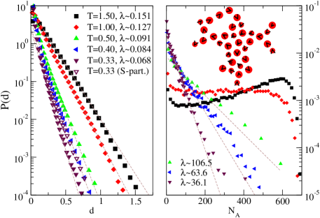
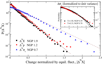
Figure 1 shows as a function of , where is , or and the denotes the change normalized by the r.m.s. equilibrium fluctuations () calculated from the time series of inherent states (=0.33). The tails are very close to exponential for . Though the distributions differ at small values, the tails for and are very similar, with the same decay length 0.16 (possibly a reflection of the strong-pressure correlations recently reported for Van der Waals systems Pedersen et al. (2008)), while that for shear is larger, 0.28. To quantify how close to Gaussian a distribution is we use a non-Gaussian parameter NGP for any quantity . This is zero for a Gaussian distribution and unity for a (symmetric) ED. The inset of the figure compares distributions of shear stress changes at the highest and lowest temperatures, now normalized to unit width. That from =1.5 is clearly more Gaussian, albeit with an exponential tail a few standard deviations from the mean.
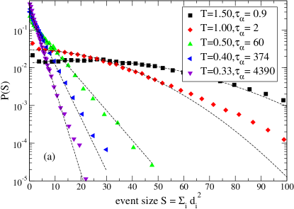
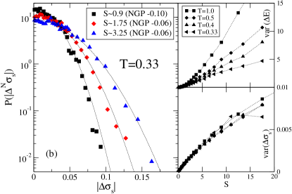
By symmetry, changes of shear stress are uncorrelated with those of energy and pressure, meaning that none of these quantities can be considered a meaningful measure of the “size” of an event. A natural measure of the size of an event is the quantity used to detect them, . The distributions are shown in Fig. 2(a). Going from high to low temperature, there is a dramatic reduction in the average size, while the shape of the distribution becomes increasingly exponential 222Note that the dynamics at the highest temperatures cannot be activated—inherent quantities decorrelate as fast as real quantities. The data is shown mainly for comparison.. Examining the distributions of for a narrow range of , we find they are Gaussian even at low when the full distributions are exponential (Fig. 2(b)). For not too large values of , (), the variance for these fixed- distributions rises approximately linearly with (right panels of Fig. 2(b)). This shows that for a given , is essentially a sum of random contributions, whose number is proportional to , the size of the event. This relationship is independent of for (lower right panel), but this holds only for small for and (upper right panel). It is not clear why this is. In all cases the variance tends to saturate as exceeds 20 (50 for at ).
The above can be made mathematically explicit by writing . At low if and the conditional probability is a Gaussian with variance , then integration gives . Linear fits to the data for =0.33 gives for the values 0.32, 1.5 and 5.8 for , and , respectively. The decay lengths of the corresponding EDs should be . For =0.33, =1.83, we get values 0.54, 0.012 and 0.023. After normalizing by the r.m.s. fluctuations as was done in Fig. 1 these become 0.16, 0.15, 0.26, in reasonable agreement with the decay lengths determined in Fig. 1.
To understand the distributions of we consider the distributions of individual (large) particle displacements in flow events, shown in Fig. 3. As found in Refs. Schrøder et al., 2000 and Vogel et al., 2004, clear exponential tails appear for larger than about 0.2. The decay lengths vary surprisingly little over the simulated temperature range, 0.08–0.15. Most of the variation is in the number of particles in the tail region (the average number per event). We find it useful to take the length scale suggested by the decay length seriously, and define the “active” particles as those with =0.1 (independent of for simplicity).
Distributions of , the number of active particles, are shown in the right panel of Fig. 3. There is a striking shift in both the shape and the mean value from high to low : A typical event at high involves most of the system; indeed, larger events are more probable than smaller ones. At low the distribution becomes exponential with a mean of order a few tens of particles. In this regime, the events are relatively localized though not necessarily compact (see the example in Fig. 3)–string-like spatial correlation is present in varying degrees in small and intermediate-sized events, while the largest events tend to have a more compact structure. The nature of spatial correlations/structure of flow events has been investigated by different authors. While Schrøder et al. found string-like correlations for transitions between minima, Appignanesi et al. used the distance matrix method to identify transitions between so-called meta-basins Appignanesi et al. (2006). Their analysis highlights events involving a large fraction of the system, which was relatively small (150 particles). In fact their data (Fig. 2 of Ref. Appignanesi et al., 2006) is consistent with an exponential tail with characteristic size of order 10-20 particles; the “democratic events” would simply be the largest events in the tail. On the other hand we observe string-like features in smaller events, but not so much in larger ones. Thus our results encompass both those of Schrøder et al. and Appignanesi et al.
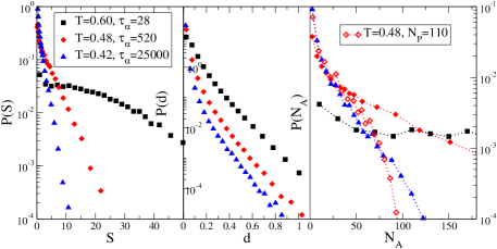
Fig. 4 shows data for a 3D system. The basic features are similar to the 2D case, and in particular the distribution controls the others. Also shown in the third panel Fig. 4 is the distribution of for a smaller system, =110, which is clearly cut off by the system size—this could well explain a factor of four difference in relaxation time between the two sizes that we observe.
The notation is meant to suggest a Lindemann-like interpretation. Several authors have emphasized the importance of such a length scale in the context of mechanical instabilities associated with structural relaxation in liquids Lubchenko and Wolynes (2007); Chakravarty et al. (2007); Dudowicz/Freed/Douglas (2005), also in experiments Schall et al. (2007). Its appearance in the present context can be interpreted as that events are in a loose sense “discretized” in units of : each event involves some number of particles each of which is displaced some number of units. Exponential distributions may be interpreted as the statement that there is no preferred number of basic units (this is analogous to a simple model for polymer size distributions, where the probability to attach a new monomer does not depend on the current length of the chain Flory (1953)).
The cross-over to exponential distributions is associated with one to well-defined localized events, whose mean size decreases with . The decrease indicates increasing material stability. A similar result was found by Fabricius and Stariolo when perturbing equilibrium configurations and comparing the corresponding inherent states Fabricius and Stariolo (2002). If event sizes decrease with decreasing temperature, this presumably has consequences for relaxation times, because a given change takes more events, although decreasing size (in particular ) also suggests that energy barriers for individual events also decrease (we will study energy barriers in upcoming work). On the other hand, when there is a distribution of barriers, there should be increased tendency for repeated reverse-transitions. This could be examined by studying correlations between events, which we have ignored here, but will address in upcoming work. One way to account for forward-backward correlations, proposed by Doliwa and Heuer Doliwa and Heuer (2003), involves grouping minima into larger structures called metabasins and study transitions between these. Their analysis indicates growing effective barriers as decreases, consistent with non-Arrhenius slowing down of dynamics. Our analysis focuses on the more fundamental units of dynamics, individual minima-transitions, because these are (in principle) unambiguously defined and it is worth understanding their statistics in detail before attempting to coarse-grain. The analysis suggests the somewhat paradoxical result that individual event barriers decrease as does. This emphasizes even more the role of correlations.
Acknowledgements.
Center for viscous liquid dynamics “Glass And Time” is sponsored by The Danish National Research Foundation.References
- Pope (1993) S. B. Pope, Annu. Rev. Fluid Mech. 26, 23 (1993).
- Dimiduk et al. (2006) D. M. Dimiduk, C. Woodward, R. LeSar, and M. D. Uchic, Science 312, 1188 (2006).
- Stanley (2003) H. E. Stanley, Physica A 318, 279 (2003).
- Bailey et al. (2007) N. P. Bailey, J. Schiøtz, A. Lemaître, and K. W. Jacobsen, Phys. Rev. Lett. 98, 095501 (2007).
- Black and Scholes (1973) F. Black and M. Scholes, J. Polit. Economy 81, 637 (1973).
- Bouchaud (2008) J.-P. Bouchaud, Nature 455, 1181 (2008).
- Cai et al. (2006) L. Cai, N. Friedman, and X. S. Xie, Nature 440, 358 (2006).
- L. and Gunaratne (2003) J. L. and G. Gunaratne, Physica A 329, 178 (2003).
- Goldstein (1969) M. Goldstein, J. Chem. Phys. 51, 3728 (1969).
- Schrøder et al. (2000) T. B. Schrøder, S. Sastry, J. C. Dyre, and S. C. Glotzer, J. Chem. Phys. 112, 9834 (2000).
- Heuer (2008) A. Heuer, J. Phys.: Condens. Matter 20, 373101 (2008).
- Miller et al. (1996) B. Miller, C. O’Hern, and R. P. Behringer, Phys. Rev. Lett. 77, 3110 (1996).
- Pratt and Dennin (2003) E. Pratt and M. Dennin, Phys. Rev. E 67, 051402 (2003).
- Büchner and Heuer (2000) S. Büchner and A. Heuer, Phys. Rev. Lett. 84, 2168 (2000).
- Adam and Gibbs (1965) G. Adam and J. H. Gibbs, J. Chem. Phys. 43, 139 (1965).
- Dyre et al. (1996) J. C. Dyre, N. B. Olsen, and T. Christensen, Phys. Rev. B 53, 2171 (1996).
- Lubchenko and Wolynes (2007) V. Lubchenko and P. G. Wolynes, Ann. Rev. Phys. Chem. 58, 235 (2007).
- Vogel et al. (2004) M. Vogel, B. Doliwa, A. Heuer, and S. C. Glotzer, J. Chem. Phys. 120, 4404 (2004).
- Powles and Fowler (1987) J. G. Powles and R. F. Fowler, Mol. Phys. 62, 1079 (1987).
- Schall et al. (2007) P. Schall, D. A. Weitz, and F. Spaepen, Science 318, 1895 (2007).
- Chaudhuri et al. (2007) P. Chaudhuri, L. Berthier, and W. Kob, Phys. Rev. Lett. 99, 060604 (2007).
- Kob and Andersen (1994) W. Kob and H. C. Andersen, Phys. Rev. Lett. 73, 1376 (1994).
- Stillinger (1995) F. H. Stillinger, Science 267, 1935 (1995).
- Pedersen et al. (2008) U. R. Pedersen, N. P. Bailey, T. B. Schrøder, and J. C. Dyre, Phys. Rev. Lett. 100, 015701 (2008).
- Appignanesi et al. (2006) G. A. Appignanesi, J. A. Rodríguez Fris, R. A. Montani, and W. Kob, Phys. Rev. Lett. 96, 057801 (2006).
- Chakravarty et al. (2007) C. Chakravarty, P. G. Debenedetti, and F. H. Stillinger, J. Chem. Phys. 126, 204508 (2007).
- Dudowicz/Freed/Douglas (2005) Dudowicz/Freed/Douglas, J. Phys. Chem. B 109, 21285 (2005).
- Flory (1953) P. J. Flory, Principles of Polymer Chemistry (Cornell University Press, 1953).
- Fabricius and Stariolo (2002) G. Fabricius and D. A. Stariolo, Phys. Rev. E 66, 031501 (2002).
- Doliwa and Heuer (2003) B. Doliwa and A. Heuer, Phys. Rev. E 67, 031506 (2003).
- Stoltze (1997) P. Stoltze, Simulation Methods in Atomic Scale Materials Physics (Polyteknisk Forlag, Lyngby, Denmark, 1997).
- Press et al. (1987) W. H. Press, B. P. Flannery, S. A. Teukolsky, and W. T. Vetterling, Numerical Recipes in C: The Art of Scientific Computing (Cambridge University Press, 1987), 1st ed.