DEPENDENCE OF THE MAGNETIZATION
OF AN ENSEMBLE OF SINGLE-DOMAIN PARTICLES
ON  THE  MEASUREMENT  TIME WITHIN VARIOUS EXPERIMENTAL AND COMPUTATIONAL METHODS

Abstract

The effect of a measurement time duration on the parameters of magnetization curves for an ensemble of identical noninteracting single-domain particles with equally oriented axes under the uniaxial anisotropy has been specified for different experiment modes, in particular for the cases of relaxation measurements and the continuous sweep of a static magnetic field. The relation between a blocking temperature and experiment characteristics has been found for these modes. A recursion method to calculate the magnetization reversal curves for such an ensemble of particles is proposed. By comparing the results of calculations of the magnetic properties by the recursion and Monte-Carlo methods, an algorithm to establish the relation between the equivalent measurement time and such parameters of the Monte-Carlo method as the number of steps and the value of aperture is suggested.

I Introduction

The problems of the magnetism of nanoparticles have attracted the attention of scientists for many decades. More than a half-century ago, the English physicists E. Stoner and E. Wohlfarth developed a simple model of magnetization reversal for uniaxially anisotropic single-domain particles at $T=0$ K [1]. According to this model, during the reversal, all spins in each particle turn in such a way that they remain parallel to each other all the time, i.e. the absolute value of the magnetic moment for each particle remains constant, and only a mutual orientation of the magnetic moments of various particles changes. In such a case, the energy of the ensemble of particles depends only on one collective variable, for example, on a total magnetization vector. Within the frame of this model, all the particles constituting a sample are assumed to have the same shape, volume $V$, and orientation of the crystallographic anisotropy axes. The volume fraction $f$ of these single-domain particles in a specimen is sufficiently small and, thus, the interparticle interaction can be neglected. The objects, whose behavior corresponds to this model, are small (in order to satisfy the condition for them to be single domains) magnetic particles (see, for example, [2]) placed in a nonmagnetic metallic or dielectric matrix.

The density of magnetic energy $U$ for a sample can be represented as the sum of the energy density of a magnetic anisotropy, which includes the anisotropy caused by demagnetization fields (a shape-dependent anisotropy term) and that of the interaction of the magnetic moment with an external field $H$. In the simplest case of a uniaxial anisotropy with regard for the first anisotropy constant only, the density of magnetic energy has the form

$$U={\frac{{f}}{{N}}}{\sum\limits_{i=1}^{N}{U_{i}}}\text{,}$$ (1)

where

$$U_{i}=-K\cos^{2}(\theta_{i}-\theta_{1})-mH\cos(\theta_{i}).$$ (2)

Here, $U_{i}$ is the density of magnetic energy for the separate $i$-th particle, $N$ is the number of magnetic particles in the sample volume, $K$ is the first constant of the uniaxial anisotropy of a particle, $m$ is its magnetization, $\theta_{i}$ is the angle between the magnetic moment of the $i$-th particle and the magnetic field direction, and $\theta_{1}$ is the angle between the easy magnetization axis of a particle (for all the particles its direction is assumed to be identical) and the magnetic field direction. For a sample which resides without an external magnetic field as long as possible, the total magnetization $M$ will turn to zero, since the numbers of particles with the magnetic moments oriented in parallel and antiparallel to the easy magnetization axis equal each other. On the contrary, the value of magnetization becomes finite upon the application of a magnetic field to the ensemble of particles. Hence, in the case where the observation duration of such the ensemble is infinitely long, its behavior will be characteristic of a paramagnet, in spite of the fact that the particles are ferromagnetic.

Neel [3] and Brown [4] took the fact into consideration that a drastic removal of the magnetic field from the ensemble of single-domain particles results in a time decay of the residual magnetization $M(t)$ according to the exponential law:

$$M(t)=M(0)\,\exp\left({-{\frac{{t}}{{\tau}}}}\right),$$ (3)

where $M(0)$ is the magnetization value at the initial time moment and $\tau$ is the relaxation time. The latter characterizes the thermally activated reversal of the direction of the magnetic moment of a separate particle between two possible minima of its potential energy. The hopping probability obeys the Arrhenius law which yields

$$\tau={\frac{{1}}{{\nu_{0}\left({\exp\left({-{\frac{{E_{mb}-E_{m1}}}{{kT}}}}\right)+\exp\left({-{\frac{{E_{mb}-E_{m2}}}{{kT}}}}\right)}\right)}}},$$ (4)

where $k$ is the Boltzmann constant, $T$ is the temperature, and $E_{m1}$, $E_{m2}$, and $E_{mb}$ are the energies for two minima and a barrier between them, respectively. The expressions for these energy values contain the product of the particle volume $V$ and the corresponding energy density $U_{i}$ which is dependent on the relative orientation of the particle magnetic moment and the field. As a result, the relaxation time $\tau$ strongly depends on the particle volume, temperature, and the value of the applied magnetic field. If the magnetic field is zero, the energy minima are equally deep. The application of a finite field makes the energy of one of them increase, while that of another one decrease. In a strong magnetic field, when the particle’s Zeeman energy exceeds that of the uniaxial anisotropy, the higher-energy minimum disappears. For the magnetic particles under discussion, the typical values of the preexponential factor $\nu_{0}$ in (4) are between $10^{8}$ and $10^{10}$ s^-1.  In the Arrhenius law, this factor is called “the attempt frequency”. For estimations, its value can be assumed to equal the precession frequency for the magnetic moment in an effective magnetic field. Neel named these materials, which are the independent single-domain magnetic particles, superparamagnets and called their quasiparamagnetic behavior as superparamagnetism.

For the superparamagnets, the shape of magnetization curves strongly varies, depending on the duration $t$ of the measurement process (measuring time). For each chosen value $t$, a blocking temperature $T_{b}$ can be introduced, which divides the whole region of temperatures into two ones with different magnetization behaviors. For one of them, the hopping, which occurs during the measuring time, of the particle magnetic moments between two energy minima should necessarily be taken into account. But, for the second one, these effects are not essential and, thus, can be neglected. It is suitable to choose the temperature, at which the temperature-dependent relaxation time $\tau$ becomes equal to the measuring time $t$, as a blocking temperature. For $T\gg T_{b}$, the measuring time $t\gg\tau$, and the magnetic moment of a particle has enough time to make multiple jumps between the energy minima. As a result, the populations of these minima do not differ from the equilibrium ones and the behavior of such a system of particles will be close to that of the ensemble of paramagnetic atoms, which is characterized by the absence of magnetization hysteresis. In this case, the magnetization of the ensemble of particles can be described by formula

$$M(H)=f\,\overline{m(H)},$$ (5)

where the time-averaged particle magnetization, which is identical for all the particles, equals

$$\overline{m(H)}={\frac{{m}}{{{\int\limits_{-\pi}^{\pi}{\exp\left({-{\frac{{U_{i}V}}{{kT}}}}\right)}}d\theta_{i}}}}\quad{\int\limits_{-\pi}^{\pi}{\exp\left({-{\frac{{U_{i}V}}{{kT}}}}\right)\cos(\theta_{i})}}d\theta_{i}.$$ (6)

The short-time measurements, for which $t<\tau$, correspond to $T<T_{b}$. In this case, there is no enough time for the transitions between the energy minima to occur, and the equilibrium populations for the states with different orientations of the magnetic moments of particles are not achieved during the measuring time. The system is in a metastable state and the curves of magnetization reversal display the hysteresis. The coercivity $H_{c}$ depends on the measuring time, anisotropy energy, and temperature. For the ensemble of uniaxial single-domain particles, Neel and Brown suggested a simple formula which connects these three parameters:

$$H_{c}(T)=H_{c}(0){\left\{{1-{\left[{{\frac{{kT\ln(t/t_{0})}}{{E_{0}}}}}\right]}^{1/\alpha}}\right\}}\text{,}$$ (7)

where $t_{0}=\nu_{0}^{-1}$, $E_{0}=KV$ is the height of the energy barrier between the two minima at $H=0$, and the exponent $\alpha$ is the parameter which depends on the orientation of a magnetic field relative to the easy axis of magnetization. For the case of the ensemble of uniaxial particles, whose easy axes are aligned along the magnetic field, $\alpha=2$.. For an arbitrary, but identical for all the particles, orientation of easy axes (with respect to the magnetic field direction), $\alpha$ is given as (see [5])

$$\alpha=0.86+1.14\left({(\cos^{2/3}(\theta_{1})+\sin^{2/3}(\theta_{1}))^{-3/2}}\right).$$ (8)

If the directions of the particles’ easy axes are uniformly distributed over the space, $\alpha=4/3$.

In the literature sources, for the case of $\alpha=2$, one can often find a representation of formula (7) in the form

$$H_{c}(T)=H_{c}(0)\left({1-\sqrt{T/{T_{{}_{b}}^{\text{NB}}}}}\right),$$ (9)

where

$$T_{b}^{\text{NB}}=\frac{KV}{k\ln(t/t_{0})}$$ (10)

is the blocking temperature in the Neel–Brown approximation. It is worth noting that, depending on the form of the anisotropy energy definition in the above expressions, the anisotropy constant $K$ can appear with a factor of 2. In spite of a relative simplicity, formulas (7) – (9) successfully discribe experimental results.

As was shown in work [6], formulas (7) – (9) can be supplemented with the expression accounting for the dependence of the particle saturation magnetization on temperature. This will result in a deviation of these expressions from the power dependence for the temperatures which are too close to the Curie temperature of ferromagnetic particles. The further improvements are reduced to the account of the distribution of particles over sizes or anisotropy values or the account, in various approximations, of a magnetic dipole-dipole interaction between the particles.

However, the analytical calculation of the magnetization hysteresis curves for the systems under consideration meets serious difficulties even for a minimal number of independent parameters. At the same time, the power of modern computer systems makes it possible to carry out such calculations by numerical methods. One of the difficulties, which arise when one carries on the numerical calculations and tries to compare their results with experiment, is related to the correctness of the identification of a measuring time $t$, which appears in calculations, with a real duration of experiment. This implies that a relevant “protocol” of measurements should be taken into account.

In modeling the properties of the ensembles of magnetic nanoparticles, the method of Monte–Carlo (MC) [7–12] has gained a significant popularity. However, this method does not include the “ real” measuring time. Instead of it, the MC method contains such parameters as the number of mathematical iterations (MC steps) and the magnitude of angular aperture used to update the magnetization direction. At the same time, the literature sources known to us do not contain an explicit relation between these parameters of the MC method and the equivalent measuring time, which corresponds to these calculations. In a few works (see, for example, [10, 13]), to correlate the number of MC steps with the measuring time, the results of MC calculations are compared with the data of actual magnetostatic measurements. The conclusions of these works are reduced to that the number of MC steps, being optimal from the viewpoint of the likelihood of the results obtained and the reasonable duration of calculations, corresponds to unrealistically short measuring times in real experiments, even for the calculations carried out with the use of high-performance modern computers. Though a number of papers devoted to this problem has been published for the last decade, the methods how to establish the correspondence between the equivalent measuring time and MC simulation parameters remain ambiguous.

It should be noted that the calculation, which would be able to account for the mode of carrying out the experiment, of the magnetization curves for the ensemble of single-domain particles has remained a problem, for a solution of which various approaches continue to be proposed (see, for example, [14, 15]).

A method developed in this work for the modeling of the magnetization curves doesn’t suffer from the above disadvantage. In what follows, we call it a recursion method (RM). In the literature sources, we haven’t met any examples of the use of such a method. Its adequacy is grounded on the favorable outcome of the comparison of its results with those of both the MC simulations and basic formulas of the Neel–Brown model [3,4] described above. Basing on such comparison, we will be able to establish a specific relation between the parameters of MC simulation (the number of MC steps and the magnitude of angular aperture) and the measuring time which corresponds to these parameters. The method we offer is suitable for the analysis of the magnetization curves for superparamagnetic systems consisting of uniaxially anisotropic particles and comprises the cases where the anisotropy axes are either parallel to each other or randomly oriented. There are no restrictions on its utilization to the modeling of the behavior of uniaxial systems with a nonzero second anisotropy constant and even the systems with a cubic anisotropy. However, to simplify the analysis, the modeling is carried out, in what follows, for the ensemble of uniaxial particles, whose axes are aligned in parallel to the magnetic field direction ($\theta_{1}=0$) with regard for only the first anisotropy constant.

II Dependence of Blocking Temperature on Measuring Time for Various Measurement Protocols

Consider an ensemble of identical noninteracting spherical single-domain particles, each of which has volume $V$ and is characterized by the uniaxial crystallographic anisotropy. We assume that the easy axes of particles are aligned in parallel to the external magnetic field, i.e. we choose $\theta_{1}=0$. We take only the first anisotropy constant into account. Let us rewrite formula (2) in terms of dimensionless units by carrying out a division of its left and right parts by the anisotropy constant $K$

$$U_{{\rm red}}=-\cos^{2}(\theta)-2h\cos(\theta),$$ (11)

where $h=Hm/(2K)$ is the dimensionless magnetic field. Here and below, the index $i$ in the notations of the energy density for a separate particle and the angle characterizing the direction of its magnetic moment will be omitted. The parameter $T_{\rm red}=kT/(KV)$ is used as a dimensionless temperature. Let us also give the definition of the dimensionless measuring time $t_{\rm red}=t\nu_{0}$, where $\nu_{0}$ is the parameter which has a frequency dimension [see expression (4) for the probability of the thermally activated reversal of particle magnetic moments] and $t$ is a real measuring time in seconds.

For the fields $h\in(-1,1)$, the solutions of the equation $\frac{\partial U_{\rm{red}}}{\partial\theta}=0$ give us the coordinates of two energy minima: $\theta_{m1}=\pi$ and $\theta_{m1}=0$. The barrier between these minima is observed at $\theta_{b}=\arccos(-h)$. The reduced energies corresponding to these angles are $E_{1}=(-1+2h)$, $E_{2}=(-1-2h)$, and $E_{b}=h^{2}$. Substituting these quantities into formula (4), the expression for the dimensionless relaxation time $\tau_{\rm red}$, which characterizes the thermally activated jumps between these minima, can be written as

$$\tau_{\rm red}={\frac{{1}}{{\exp}\left[{-\left({h-1}\right)^{2}/T}_{\rm red}\right]{+\exp}\left[{-\left({1+h}\right)^{2}/T}_{\rm{red}}\right]}}.$$ (12)

As was noted above, the blocking temperature $T_{b}$ depends on the measuring time $t_{\rm red}$. It is seen that the use of the condition $t_{\rm red}=\tau_{\rm red}(T_{\rm red}=T_{b}^{r})$ for the determination of the relaxation time leads to the relation

$$T_{b}^{r}=1/\ln(2t_{\rm red}).$$ (13)

Here, $T_{b}^{r}$ is the blocking temperature in a zero magnetic field taken in the dimensionless form defined above. This expression doesn’t coincide with that for the blocking temperature in the Neel–Brown approximation, $T_{b^{\ast}}^{r}$ (a reduction of $T_{b}^{\rm{NB}}$ determined from expression (10) to a dimensionless unit results in $T_{b^{\ast}}^{r}=1/\ln(t_{\rm red})$). Thus, the Neel–Brown approximation corresponds to neither the condition $t=\tau(T=T_{b})$ (with expression for $\tau$ in the form (4)) nor this relation.

Actually, formula (9) along with expression (10) for $T_{b}^{\rm{NB}}$ can be obtained from the following considerations. In the case of high fields and low temperatures, i.e. when $h/T_{\rm red}\gg 1$, we can neglect the second exponential term in (4) (or in a dimensionless expression (12)). Let us take into account only the time, which is necessary for the thermally activated reversal of a particle magnetic moment from a metastable to the basic state, and ignore the backward jumps. In this case,

$$\tau_{\rm red}^{\ast}\approx\left\{\exp\left[-(h-1)^{2}/T_{\rm{red}}\right]\right\}^{-1}.$$ (14)

A formal extrapolation, which is not strictly accurate, of this expression to the zero magnetic field and its equating with a measuring time leads to a definition of the effective blocking temperature $T_{b^{\ast}}^{r}$ in this approximation as

$$T_{b^{\ast}}^{r}=1/\ln(t_{\rm red}),$$ (15)

i.e. to the formula which was obtained by means of reduction of (10) to the dimensionless units. It is seen that $T_{b}^{r}$ (see (13)) and $T_{b^{\ast}}^{r}$ (see (15)) are connected by a simple relation $(T_{b^{\ast}}^{r})^{-1}=$ $(T_{b}^{r})^{-1}-\ln(2)$.

The most important point in the approximation [3,4] is probably the expression for the temperature dependence of coercivity [see (7) and (9)]. At low temperatures, the criterion $h/T_{\rm red}\gg 1$ can already be fulfilled for a coercive field ($h=h_{c}$) and, thus, approximation (14), along with the definition, which follows from it, of the blocking temperature, i.e. $T_{b^{\ast}}^{r}$ becomes justified.

Consider the question as to which type of experimental data and measurement mode corresponds the Neel–Brown approximation in more details. Expression (9) with definition (10) [or (12) in dimensionless units] for a blocking temperature can be obtained proceeding from the assumption that the field which corresponds to coercivity is the one, for which $\tau_{\rm red}(h=h_{c})=t_{\rm red}$. Then the relation

$$t_{\rm red}\;\approx\left\{\exp\left[{-{\frac{{\left({h_{c}(T_{\rm{red}})-1}\right)^{2}}}{{T_{\rm red}}}}}\right]\right\}^{-1}$$ (16)

will be valid for the low temperature region of the coercivity vs temperature dependence. After taking the logarithm on both left and right parts of (16), we obtain the expression for the temperature dependence of coercivity:

$$h_{c}(T_{\rm red})=\;1-\sqrt{T_{\rm red}\ln\,(t_{\rm red})}.$$ (17)

Defining a blocking temperature as that, at which the extrapolation of a low temperature part of the temperature dependence of coercivity with either formula (9) or (17) reaches zero value for a preset measuring time, we can write the expression for the temperature dependence of coercivity as

$$h_{c}(T_{\rm red})=1-\sqrt{T_{\rm red}/T_{b^{\ast}}^{r}},$$ (18)

where $T_{b^{\ast}}^{r}$ is determined from formula (15).

However, one should keep in mind that, to derive Eq. (18), we had to use assumption (16) which is not completely accurate in the strict sense. Moreover, it should be remembered that, to obtain (15), we used one more approximation which consisted in the extrapolation of the low-temperature high-field part of the $\tau_{\rm red}^{\ast}$ vs $h$ dependence to the zero field. In fact, the measuring time, which goes into these equations, can be interpreted as the time, during which the system relaxes from the magnetosaturated state after the instantaneous switching-on of the given field. Such a definition of the measuring time is related to the relaxation measurements. For the relaxation experiments under consideration, the time dependence of the magnetization is given as

$$M(h,t_{\rm red})=M_{\rm equ}(h)+(M_{0}{\rm sign}(h_{\rm satur})-$$

$$-M_{\rm equ}(h))\exp\left(-{\frac{{t_{\rm red}}}{{\tau(h,T_{\rm red})}}}\right).$$ (19)

Here, $M_{\rm{equ}}(h)$ is the equilibrium magnetization in a field $h$, which for the system under study is determined as $M_{\rm{equ}}(h)=M_{0}\tanh(2h/T_{\rm red})$, sign$(h_{\rm{satur}})$ is the sign of the saturation field, and $M_{0}$ is the saturation magnetization. At the same time, the coercivity is determined from the condition $M(h_{c},t_{\rm{red}})=0$ which differs from the condition $t_{\rm red}=\tau_{\rm{red}}(h_{c},T_{\rm red})$. The latter, perhaps, might be used as an approximate condition. At low temperatures and sufficiently high coercivities (when $h_{c}/T_{\rm red}\gg 1$, which is a criterion of the applicability of approximation (14)), it is either a relation $\exp\left[-t_{\rm red}/\tau_{\rm{red}}(h_{c},T_{\rm red})\right]\approx 1/2$ or $t_{\rm red}=\tau_{\rm{red}}(h_{c},T_{\rm red})\ln(2)$ that would better satisfy the requirement $M(h_{c},t_{\rm red})=0$. Thus, we will use them instead of (16). The utilization of such an approximation makes it possible to obtain the equation for the temperature dependence of coercivity. This equation has the same form as formula (9), in which the effective blocking temperature $T_{b^{\ast}}^{r}$ is substituted by $T_{b^{\ast\ast}}^{r}$. The latter coincides with neither (10) nor (15); it equals

$$T_{b^{\ast\ast}}^{r}=\;{\frac{{1}}{{\ln\,[t_{\rm red}/\ln(2)]}}}={\frac{{1}}{{\ln(t_{\rm red})-\ln[\ln(2)]}}}\rm{.}$$ (20)

It is seen that $(T_{b\ast\ast}^{r})^{-1}=$ $(T_{b\ast}^{r})^{-1}-{\ln[\ln(2)]=}T_{b}^{r}-{\ln(2)-\ln[\ln(2)]}$.

To correctly determine $T_{b}$ and obtain the expression for the coercivity vs $T$ dependence, one should not only find the measuring time, but also take the measurement protocol for the magnetic characteristics of a system of particles into account.

Consider the relaxation experiments where the saturating magnetic field, which acts on the system, is instantaneously (or rapidly enough in real conditions so that $t\ll\tau$) transformed into some other field $h$, after which the system relaxes with time. In this case, let the measurements of the magnetization be continuously carried out during a time interval $t_{\rm{red}}$. Consider the ways of the determination of both $T_{b}^{r}$ [see (13)] and the effective blocking temperature $T_{b^{\ast}}^{r}$ [see (18)] to make it possible to specify the temperature dependence of coercivity. It is pertinent to take a temperature at which $\tau_{\rm red}(h=0)=t_{\rm red}$ [with regard for (12) for $\tau_{\rm red}$] as $T_{b}^{r}$. If this condition is fulfilled, the zero-field magnetization (the so-called remanent magnetization) has to be $e$ times less than the saturation magnetization (here and below, the number $e$ means the base of the natural logarithm). To measure the coercivity according to this method and to determine the blocking temperature from the $h_{c}(T_{\rm red})$ dependences, it is necessary at each measurement temperature and at a certain field which has the opposite sign relative to the initial saturation field, to record a time point, at which the magnetic relaxation curve crosses the zero value. The corresponding field will equal the coercivity at the given values of temperature and measuring time. At low temperatures, it will correspond to the solution of the equation

$$t_{\rm red}=[\exp\,\left({-{\frac{{\left({1-h_{c}(T_{\rm red},t_{\rm red})}\right)^{2}}}{{T_{\rm red}}}}}\right)+$$

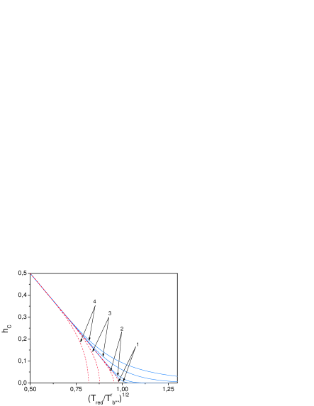
Figure 1: Temperature dependences of coercivity calculated for different measuring times: $t_{\rm red}=4$, $10$, $10^{3}$, and $10^{7}$ for the pairs of curves 1, 2, 3, and 4, respectively. Dashed and solid lines represent the solutions of Eq. (21) and $M(h_{c},t_{\rm red})=0$, respectively.

$$+\exp\,\left({-{\frac{{\left({1+h_{c}(T_{\rm red},t_{\rm red})}\right)^{2}}}{{T_{\rm red}}}}}\right)]^{-1}\ln 2.$$ (21)

Then, for each value of $t_{\rm red}$, one should plot the dependence $h_{c}(T_{\rm red})|_{t_{\rm red}}$ and find $T_{b\ast\ast}^{r}(t_{\rm{red}})$ from the approximation of its low temperature part by formula (18), in which $T_{b\ast\ast}^{r}$ substitutes for $T_{b\ast}^{r}$. A solution of Eq. (21), which describes the temperature dependence of coercivity, can be found only numerically. As was noted above, it gives a correct criterion for the determination of $h_{c}(T_{\rm{red}},t_{\rm red})$ only for the temperatures lower than $T_{b\ast\ast}^{r}$. To find the temperature dependence of $h_{c}$ over the whole range of temperatures, it is necessary to solve the equation $M(h_{c},t_{\rm{red}})=0$ with the use of expressions (12) and (19) for $\tau_{\rm red}$ and $M(h,t_{\rm red})$, respectively. It should be noted that the $h_{c}(T_{\rm red})$ dependence found in such a way doesn’t exhibit a sharp break by turning into zero at the blocking temperature. On the contrary, it diminishes smoothly over a certain temperature range above the blocking temperature.

Figure 1 shows the temperature dependences of coercivity for various measuring times $t_{\rm red}$ calculated by means of the numerical solution of Eq. (21) and the equation $M(h_{c},t_{\rm red})=0$ with the components described above. The quantities $\sqrt{T_{\rm red}/T_{b\ast\ast}^{r}(t_{\rm red})}=\sqrt{T_{\rm red}\cdot\left\{\ln(t_{\rm{red}})-\ln\left[\ln(2)\right]\right\}}$ are taken as the units of the abscissa axis.

As is seen from the figure, all the curves coincide with each other at low temperatures. Extrapolation of the low temperature branches to higher $x$ values gives $\sqrt{T_{\rm red}/T_{b\ast\ast}^{r}(t_{\rm red})}=1$. However, the real curves do not follow the extrapolated one. On the contrary, they diverge to different sides in the vicinity of the effective blocking temperature. The curves obtained from Eq. (21) turn into zero below $T_{b\ast\ast}^{r}$, while those obtained from the condition $M(h_{c},t_{\rm red})=0$ diminish smoothly above $T_{b\ast\ast}^{r}$. For very great values of $t_{\rm red}$ ($t_{\rm red}>10^{5}$), the curves remain linear practically to $T_{b\ast\ast}^{r}$. It should be noted that, taking $\nu_{0}\approx 10^{8}\div$ $10^{10}$ s^-1 into account, only such values of $t_{\rm red}$ are characteristic of real measurements. The shorter the measuring time, the lower is the temperature, at which the curves start to deviate from the linear law which corresponds to formula (18) where the effective blocking temperature equals $T_{b\ast\ast}^{r}$. At the same time, both the temperature smearing of a sharp transition in the vicinity of $h_{c}=0$ and the transition retention to the temperatures above the blocking temperature disguises a deviation of the blocking temperature from $T_{b\ast\ast}^{r}$ at short (almost unlikely in practice) measuring times. For this reason, if one employs the relaxation method to measure a coercivity, the deviation from formula (18), in which $T_{b\ast\ast}^{r}$ serves as the effective blocking temperature, will appear only in the form of the aforementioned smearing. The temperature smearing of the transition, which is observed as $h_{c}$ tends to zero, seems to be natural, since the hysteresis is a manifestation of the metastability at a finite measuring time. Such a hysteresis will occur, to a greater or lesser extent, at any finite temperatures. It is worth noting that the coercivity, even being negligibly small at $T>T_{b}$, doesn’t turn into zero.

In principle, the relaxation measurement protocol considered above is used in practice. However, the protocol of the continuous sweep of a magnetic field (CSMF) with certain rate is more often used for magnetostatic measurements. In the course of its implementation, the relaxation of the magnetization to its equilibrium value occurs in a magnetic field, which continuously changes. The case where the sweeping rate is infinitely small corresponds to the infinitely great measuring time. In this case, the system is in an equilibrium state, and such a case corresponds to $T_{b}\rightarrow 0$. For the regions where superparamagntism becomes clearly apparent and $T_{b}\neq 0$, the sweeping rate becomes comparable with the relaxation time $\tau$. Under these conditions, the concept of a measuring time should be made more specific and related to the experiment conditions and the blocking temperature definition.

In the case of the CSMF studies, the simplest and natural way to analyze and describe the system properties may be the analysis of a hypothetical protocol of measurements, in which the whole range of the field sweep is divided into equal intervals. In this case, the magnetic field sweep can be regarded as a series of jumps, each of which being characterized by a specific waiting time $t_{w}$ after the previous jump. In this case, the magnetization for each field point will relax during $t_{w}$ from the value at the previous point. Such a method can be called as recursive, since, in order to describe the magnetization relaxation at the $n$-th field point, one should reconstruct a successive series of magnetization relaxations for all $n-1$ previous points. In the limit where the interval between successive points tends to zero, we obtain the CSMF protocol. It is appropriate to define the measuring time as a sweep time for the unit field interval (taken in dimensionless units), i.e. to define $t_{\rm red}$ as the quantity which is reciprocal to the sweep rate averaged over the whole intervals.

Figure 2 shows the dependences of the blocking temperatures defined in different ways on $1/\ln(t_{\rm red})$: $T_{b}^{r}$ was obtained from expression (13), while $T_{\rm{b-scan}}^{r}$ was calculated numerically by means of the RM for different values of $n$, where $n$ is the number of intervals, into which the unit field interval $\Delta h=1$ was divided. In calculations, the $T_{\rm{b-scan}}^{r}$ was regarded as a value of the reduced temperature, at which the remanent magnetization was $e$ times less than the saturation magnetization.

It is seen that all dependences, which are calculated with the use of the RM, lie between two curves, one of which is the curve obtained from (13), while the other is some limiting curve, to which the calculated results tend when $n$ goes to infinity. This curve corresponds to the CSMF case. It is clear that the solution corresponding to $n=1$, i.e. when one point falls on a unit interval, coincides with that obtained from formula (13). One can see that the results start to diverge from the limiting solution already for $n\sim 200$.

The dependences $h_{c}(T_{\rm red})$ were also calculated for the case $n\rightarrow\infty$. Extrapolation of their low temperature regions to the temperatures where $h_{c}\rightarrow 0$ resulted in the same dependences of $T_{\rm{b-scan}}^{r}(t_{\rm red})$ as those which were determined from the expression for the remanent magnetization. For all $t_{\rm red}$ values, except for the shortest ones ($t_{\rm red}<5$), the curves $h_{c}(T_{\rm red})$ correspond to Eq. (18), in which $T_{\rm{b-scan}}^{r}(t_{\rm red})$ substitutes for $T_{b\ast}^{r}$.

The analysis of the data in Fig. 2 shows that the CSMF case is the limiting case of relaxation measurements when the measuring time is reduced. In fact, in the former case, the system resides in the saturated state for a considerable part of the sweep time which falls on a unit field interval. The effective sweep time from the saturating field to the zero  (or  coercive)

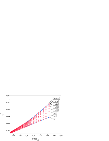
Figure 2: The $T_{\text{b-scan}}^{r}(t_{\rm red})$ dependences calculated by the RM technique for various numbers of points per unit field interval (circles). The top solid line corresponds to the limiting case $n\rightarrow\infty$. The bottom line shows the $T_{b}^{r}(t_{\rm red})$ dependence calculated by formula (13)

one turns out to be far shortest than $t_{\rm red}$ defined above for the CSMF protocol. For this protocol, one can introduce the effective measuring time $t_{\rm red}^{\rm{eff}}$, at which $T_{\rm{b-scan}}^{r}(t_{\rm red})$ in the CSMF case will coincide with $T_{b}^{r}(t_{\rm{red}}^{\rm{eff}})$ in the case of relaxation measurements, i.e. it will equal $1/\ln(2t_{\rm red}^{\rm{eff}})$. It is appropriate to regard such time as the sweep period for the field, at which the equilibrium magnetization changes from zero to a certain value $aM_{0}$. Then, from the fitting of the limiting curve in Fig. 2, we should find the optimal value of $a$ (its expected value is about 2). Such an approach leads to the equation $t_{\rm{red}}^{\rm{eff}}=t_{\rm red}$arctg $h(a)/\left[2\ln(2t_{\rm{red}}^{\rm{eff}})\right]$, whose solution is

$$t_{\rm red}^{\rm{eff}}(t_{\rm red},a)={\frac{{t_{\rm red}}\,\rm{arctanh}\,(a)}{2W\left[{t_{\rm red}}\,\rm{{arctanh}}\,{(a)}\right]}}\rm{.}$$ (22)

Here, $W(x)$ is the so-called Lambert $W$-function which is a reciprocal function to $x=W(x)\exp(W(x))$. This function was introduced into mathematical physics relatively recently [18]. In a number of cases, for example in a popular program “Mathematica” developed by “Wolfram Research” company, it is denoted as “ProductLog”. The examples of the solution of various tasks of mathematical physics with the use of this function are presented in [19].

The calculations we carried out have shown that the expression

$$T_{\rm{b-scan}}^{r}(t_{\rm red})=1/\ln\left[2t_{\rm red}^{\rm{eff}}(t_{\rm red},a=0.45167)\right]$$ (23)

approximates the limiting curve of Fig. 2 with a high precision. Noticeable deviations are observed only for the smallest $t_{\rm red}$ values ($t_{\rm{red}}<5$), which are of minor importance from the practical point of view. Thus, this approximation requires only one fitting parameter $a$.

Taking into account that the $W(x)$ function is not widely used in the scientific literature, we also found the approximation of the limiting curve for $T_{\rm{b-scan}}^{r}(t_{\rm red})$ by a power series of $\left[\ln(2t_{\rm red})\right]^{-1}$:

$$T_{\rm b-scan}^{r}(t_{\rm red})={\frac{{1}}{{\ln\,(2t_{\rm red})}}}\times$$

$$\times\left({1+a_{0}+{\frac{{a_{1}}}{{\ln\,(2t_{\rm red})}}}+{\frac{{a_{2}}}{{[\ln\,(2t_{\rm red})]^{2}}}}+{\frac{{a_{3}}}{{[\ln(2t_{\rm red})]^{3}}}}.....}\right)$$ (24)

with four fitting parameters: $a_{0}=0.01$, $a_{1}=5.197$, $a_{2}=-3.581$, and $a_{3}=-1.602$. Finally, we note that, in real CSMF experiments, ${t_{\rm red}}$ is usually between $10^{10}$ and $10^{14}$. For this reason, the discrepancies in the determination of a blocking temperature are almost unnoticeable for different measurement methods.

III Recursion Method

Before turning to a description of the calculation method for magnetic reversal curves for different measuring times, it should be noted that its implementation, as also in the case of MC modeling, requires some efforts in the programming of a calculation procedure. We will use the same dimensionless parameters as in Section 2: $h=Hm/(2K)$ is the magnetic field, $t_{\rm red}=t\nu_{0}$ is the measuring time, $T_{\rm{red}}=kT/(KV)$ is the temperature, $n$ is the number of points per unit field interval, and $\overline{m_{\rm red}}=f\overline{m}/(fm_{s})=M_{\rm red}$- is average magnetization for measuring time, which normalized on a saturation magnetization $m_{s}$.

The method is based on the following prerequisites.

1. The hysteresis, which is a result of the metastability, will become apparent at a finite measuring time only if the state of a system is characterized by two minima in the dependence of its energy on the orientation of a particle magnetic moment. The hysteresis originates from the metastability with regard to thermally activated jumps over a potential barrier. In its turn, the metastability appears as a result of the finiteness of a measuring time.

2. In real magnetostatic measurements, the ratio of a barrier energy at $H=0$ to a thermal energy, at which the deblocking of a magnetic moment occurs, is near 25. That is why we assume that, even at temperatures higher than the blocking temperature, the orientation of a magnetic moment will be localized in one of the minima, rather than smeared by temperature over a wide range of angles $\theta$.

3. To determine the magnetization of a system, the concept of potential well (minimum) populations is introduced. This concept is based on the distribution statistics of magnetic moment directions in an infinitely great ensemble of identical and equally oriented particles.

4. In dimensionless units, the magnetization of the system depends only on the coordinates of minima ($\theta_{m1},\theta_{m2}$) and their populations ($N_{1},N_{2}$): $M_{\rm red}=N_{1}\cos(\theta_{m1})+N_{2}\cos(\theta_{m2})$.

The limits of applicability of this method will be discussed later on; we will concentrate now only on the calculation procedure.

We reduce formula (2) for the density of energy of a separate particle to that in the dimensionless units (the index $i$, which refers to the number of a particle, will be omitted again, as was done in (11)):

$$U_{r}=-\cos^{2}(\theta-\theta_{1})-2h\cos(\theta).$$ (25)

Consider the energy profile $U_{r}$ in the phase space $\theta\in(-\pi,\pi]$ as a function of the magnetic field $h$. The energy minimum will correspond to the equilibrium orientation of the magnetic moment. The number of extrema can be found by solving the equation $\partial U_{r}/\partial\theta=0$. Substituting the roots of this equation into the expression $\partial^{2}U_{r}/\partial\theta^{2}$, we can find out if a given root corresponds to the energy minimum or maximum.

The method developed consists of a few successive steps. At first, the system is assumed to reside in a saturating magnetic field. Then we sequentially change the field to smaller values and calculate the magnetization, to which the system will come during the time interval which is equal to the period of the system residence at a certain field point $h_{k}$. The relaxation time is determined by the form of the potential in a field $h_{k}$. According to this method, the calculations should start from a negative field, which is high enough so that the energy displays only one minimum, and finish at a sufficiently high positive field, for which the energy again displays only one minimum. Thus, the calculation procedure can tentatively be divided into three stages.

The first stage is applicable when the field is negative and the state of the system is characterized by only one energy minimum. This stage includes:

1. Determination of the total number of extrema in the range $\theta\in(-\pi,\pi]$ and their separation into minima and maxima.

2. If the state of the system is characterized by only one energy minimum, then $N_{1}=1$ and $N_{2}=0$, and the magnetization equals $M_{\rm{red}}=N_{1}\cos(\theta_{m1})+N_{2}\cos(\theta_{m2})$. If there are two minima, we should go on to the second stage.

3. Recording the magnetization for a given field point $h_{k}$, changing the field to $h_{k+1}=h_{k}+\Delta$, and going on to item 1.

The second stage is applicable when the state of the system is characterized by two energy minima and includes:

4. Determination of the total number of extrema in the range $\theta\in(-\pi,\pi]$ and their separation into minima and maxima.

5. If the state of the system is characterized by a single energy minimum, then we should go on to the third stage. If there are two minima, a temporal evolution of $N_{1}$ and $N_{2}$ should be considered. This includes:

a) determination of the equilibrium populations $N_{1\infty}$ and $N_{2\infty}$, i.e. the values of $N_{1}$ and $N_{2}$ when the time interval is infinite:

$$N_{1\infty}={\frac{{1}}{{1+\exp}\left[{-(E}_{2}-E_{1}{)/T}_{\rm red}\right]}}\rm{,\ \ \ }N_{2\infty}=1-N_{1\infty}\rm{,}$$ (26)

where $E_{1}=U_{r}(\theta_{m1})$ and $E_{2}=U_{r}(\theta_{m2})$ are the energy values for the first and second minima, respectively;

b) tracing the relaxation of $N_{1}$ and $N_{2}$ for the time interval $t_{\rm{loc}}=t_{\rm red}/n$:

$$N_{1t}=N_{1\infty}+\left({N_{1}-N_{1\infty}}\right)\,\exp\left(-t_{\rm{loc}}/\tau_{\rm red}\right)\rm{,}$$ (27)

$$\tau_{\rm red}=\frac{1}{\exp\left[-(E_{b}-E_{1})/T_{red}\right]+\exp\left[-(E_{b}-E_{2})/T_{red}\right]}\rm{.}$$ (28)

c) recording the new values of $N_{1}$ and $N_{2}$:

$$N_{1}=N_{1t}\rm{,\ }N_{2}=1-N_{1t}\rm{.}$$

6. Calculation of the magnetization $M_{\rm red}=N_{1}\cos(\theta_{m1})+N_{2}\cos(\theta_{m2})$.

7. Fixation of the magnetization for a given field point $h_{l}$, changing the field to $h_{l+1}=h_{l}+\Delta$, and going on to item 4.

The third stage is applicable when the field is positive, and there is no second minimum. This stage includes:

8. Determination of the total number of extrema in the range $\theta\in(-\pi,\pi]$ and separation of them into minima and maxima.

9. If the state of the system is characterized by only one energy minimum, then $N_{1}=0$ and $N_{2}=1$ and the magnetization equals $M_{\rm{red}}=N_{1}\cos(\theta_{m1})+N_{2}\cos(\theta_{m2})$.

10. Fixation of the magnetization for a given field point $h_{m}$, changing the field to $h_{m+1}=h_{m}+\Delta$, and going on to item 8.

The greater $n$, the more minutely the magnetization curve will be calculated. At the same time, the real time interval spent on the measurement of the complete hysteresis loop (${\{}-h,h{\}},{\{}h,-h{\}}$) will equal $t=2t_{\rm red}\Delta h/\nu_{0}$ s, where $\Delta h$ is the interval (taken in dimensionless units) of the complete sweep of the magnetic field. If one does not need to model the partial hysteresis loops, it is enough to carry out the calculations for the interval ${\{}-h,h{\}}$, because the second interval ${\{}h,-h{\}}$ will be symmetric relative to the coordinate origin ($0,0$). To obtain the magnetization curves for an ensemble which is characterized by a distribution of some particles’ parameters, it is necessary to divide the distribution function into sufficiently small intervals and, having calculated the separate curves for each of the intervals (i.e. for the average values of a parameter in this interval), to sum them.

The inset in Fig. 3 shows the results of the modeling of magnetization curves for the ensemble of uniaxial particles, whose easy axes are aligned in parallel to the magnetic field. The calculations were made for $t_{\rm{red}}=1.25\times 10^{6}$ and $n=125$. The temperature $T_{\rm red}$ was varied from 0 to 0.02. The temperature dependence of coercivity (squares) is well described by formula (7) and has a square-root character ($\alpha=2$) for the given orientation of the particle easy axes. The plot of this curve in the form $h_{c}(\sqrt{T_{\rm red}})$ (triangles) confirms the latter fact. Such a dependence is a straight line and its extrapolation to the intersection with the ordinate axis unambiguously determines the blocking temperature $T_{b}^{\rm red}$= $(0.3\pm 0.005)^{2}$ = $0.09\pm 0.003$. At the same time, the calculation of $T_{\rm{b-scan}}^{r}(t_{\rm{red}}=1.25\times 10^{6})$ according to formulas (23) and (24) in the case $n\rightarrow\infty$ (or, at least, $n\geq 200$) gives 0.0915. Thus, the value of $T_{b}^{\rm red}$ = $0.09$ obtained from Fig. 3 well agrees with that found from (23) and (24).

The temperature dependence of the remanent magnetization $M_{r}$ normalized to the saturation magnetization exhibits a sharp rise (see Fig. 3, circles) at temperatures where $h_{c}$ becomes noticeable.

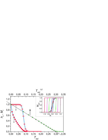
Figure 3: Results of the modeling of the $h_{c}(T_{\rm red})$ (solid squares) and $M_{r}(T_{\rm red})$ (open circles) dependences for $t_{{\rm red}}=1.25\times 10^{6}$. The $h_{c}(\sqrt{T_{\rm red}})$ dependence is shown by open triangles. The calculations are carried out for $n=125$. The inset shows the magnetization curves which correspond to these dependences, for $T_{\rm red}=0.2$, $0.1$ (anhysteretic curves) and $0.07$, $0.03$, $0.01$, and $0.00$ (with a hysteresis which consecutively widens)

As was expected, the value $T_{\rm red}=$ $T_{b}^{\rm red}=0.09$ corresponds to a decrease in the remanence by a factor of 2.718. This means that the plots of the temperature dependences of the coercivity and the remanent magnetization normalized to the blocking temperature (see expression (23) or (24)) should coincide. Figure 4,a shows the results of the RM modeling obtained on the same ensemble of particles, but for different values of the measuring time. These data replotted in the coordinates where the abscissa axis is scaled by $T_{\rm{b-scan}}^{r}(t_{\rm red})$ are presented in Fig. 4,b. It is seen that almost all the $H_{c}\left[T_{\rm red}/T_{\rm{b-scan}}^{r}(t_{\rm{red}})\right]$ curves overlap one another. Replotting these curves in the coordinates with a “rooted abscissa” shows that, at temperatures far lower than the blocking temperature, they are well described by formula (9).

A characteristic feature of the $M_{r}\left[T_{\rm red}/T_{\rm{b-scan}}^{r}(t_{\rm red})\right]$ dependence is a broadening of the front of the $M_{r}$ growth with decrease in $t_{\rm red}$. All the curves intersect one another at a point, whose ordinate equals 0.368, i.e. $1/e$. Thus, the simulated magnetization curves, as well as the $H_{c}(T_{\rm red})$ and $M_{r}(T_{\rm red})$ dependences obtained from them, are in compliance with the regularities described in Section 2, which determine their behavior over a wide range of measuring time values.

The RM calculations of the magnetization curves were also carried out for the ensembles of particles with 3D- and 2D-distributions of easy axes. The results obtained well agree with the data calculated by the MC method [1,6,7]. The fact that the time of computer calculations is much less within the RM than that within the MC method gives us an additional argument in favor of the method we have proposed here.

It is worth noting that the method developed contains a series of approximations, which can lead to some inaccuracy of the results obtained. The most important approximation is related to a failure to consider the thermal fluctuations of a magnetic moment in the vicinity of an energy minimum . This, in turn, gives rise to an inaccuracy in the determination of the magnetization at sufficiently high temperatures (or for very short values of the measuring time ($t_{\rm red}\leq 5$)). It should be stressed once more that, in the first place, the RM is used for the calculations of the ithysteresis loops of the magnetization. To study the magnetization curves itabove itthe blocking temperature, it is enough to utilize formula (5). With the use of this formula, one can also estimate the measure of inaccuracy for the magnetization calculated by the RM at temperatures higher than the blocking temperature. It is obvious that the higher the temperature, the greater is the inaccuracy. To check the role of this factor, we calculated the magnetization curves for $t_{\rm red}=1.25\times 10^{4}$ and $T_{\rm{red}}>$ $T_{b}^{\rm red}$ (namely, for $T_{\rm red}=0.2$) by the RM and formula (6). The maximal error in the determination of the magnetization did not exceed $1.5\%$. The measuring times, which are shorter than the above value, are hardly possible in practice.

IV Monte–Carlo Method

For the modeling by Monte–Carlo method, the standard algorithm suggested by Metropolis et al. [16] was used. It is known that, for a sufficiently great number of steps $N_{\rm{MC}}$, such an algorithm leads to the Boltzmann distribution. This means that a system comes to the thermodynamic equilibrium and thus, no metastability and, respectively, no hysteresis will be observed unless we introduce some special tricks. In a general case, for a great number of MC steps, the results will tend to those which can be obtained with the use of formula (5). To “catch” the metastability in the process of magnetization reversal, it is necessary to use a finite number of MC steps and restrict the generation of a trial random orientation of the magnetic moment in the vicinity of the current orientation by a certain not great aperture $\Delta\theta$, instead of the generation over the  whole  phase  space.

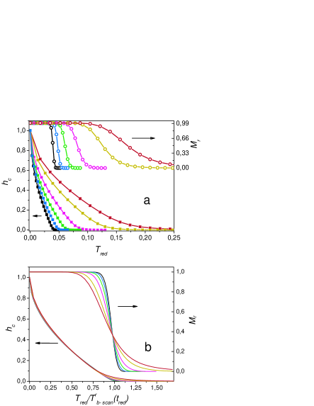
Figure 4: (a) Families of the $H_{c}(T_{\rm red})$ (solid squares) and $M_{r}(T_{\rm red})$ (open circles) curves calculated for the ensemble of particles, whose easy axes are aligned along the magnetic field, for $t_{\rm red}=2.5\times 10^{12}$, $2.5\times 10^{10}$, $2.5\times 10^{8}$, $2.5\times 10^{6}$, $2.5\times 10^{4}$, and $2.5\times 10^{3}$ ($n=250$). The curves are shifted towards the right side as $t_{\rm red}$ decreases. (b) The same curves replotted in the coordinates where the abscissa axis is scaled by $T_{\rm{b-scan}}^{r}(t_{\rm red})$

This trick is one of the standard MC techniques to model the hysteresis loops [7, 10, 12]. The procedure of modeling is divided into two stages: a thermalization of the system and a magnetization reversal process itself.

The system thermalization is regarded as the procedure consisting from tens to hundreds of thousands of MC steps at high negative fields and sufficiently high temperatures. This procedure is aimed at bringing the system to a state which is equivalent to the thermal equilibrium. To model the magnetization reversal process, one should give an increment in the magnetic field and perform a given number of MC steps for each field point. Such algorithm is widely used, and we won’t describe it in details (see its description, for example, in [10,12,17]). Here, we only note that, in our calculations, we set the aperture value $\Delta\theta=6{{}^{\circ}}$ (the role of the aperture will be discussed below). The thermalization procedure was carried out for $T_{\rm red}=0.5$, $h=-10$, and $N_{\rm{MC}}=10000$. To compare the efficiency of the MC method and RM, we performed a series of calculations of the magnetization curves for various $T_{\rm{red}}$ by both methods. To determine the blocking temperature, we utilized the extrapolation of a low-temperature region of the $h_{c}(\sqrt{T_{\rm red}})$ dependence, which is linear in these coordinates, to its intersection with the abscissa axis. In both cases, 300 field points fell on one magnetization curve ($-2<h<2$), which meant that $n$ was equal to $75$. Then we carried out the calculations of the $H_{c}(T_{\rm red})$ and $M_{r}(T_{\rm red})$ dependences according to the MC method with $N_{\rm{MC}}=5\times 10^{6}$, a measuring time $t_{\rm red}$ for the RM procedure was fitted in such a way that the dependences obtained agreed as much as possible with the results of the MC modeling.

Figure 5 presents the $H_{c}(T_{\rm red})$ and $M_{r}(T_{\rm red})$ dependences obtained by the MC method (squares and circles) and RM (solid lines) for the ensemble of particles, whose easy axes are aligned along the magnetic field. It is seen from the figure that, in spite of the disadvantages of the RM, which were formulated in Section 3, both the methods give almost identical dependences. Since the duration of the MC calculations was sufficiently long (it took 46 min to calculate one magnetization curve), only a small number of particles (5 particles in the ensemble) was taken for calculations and this resulted in a noticeable data scattering. On the contrary, it took no more than a minute to make the RM calculations for one magnetization curve. In the case under consideration, the number of MC steps at each field point was $5\times 10^{6}$, while the RM with a fitting procedure described above gave $t_{\rm{loc}}=8\times 10^{3}$, which means that, for $n=75$, $t_{\rm red}=nt_{\rm{loc}}=6\times 10^{5}$. Since the parameter $\nu_{0}$ is of the order of $10^{8}-10^{11}$, the actual measuring time for such a kind of the MC procedure corresponds to $10^{-4}-10^{-7}$ s. This is, of course, an extremely small time interval. At the  same  time,  it  is  pertinent  to  specify  the interrelation between the number of MC steps and the aperture, on the one hand, and the  real  time  interval,

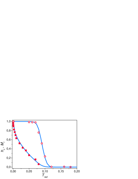
Figure 5: Dependences $H_{c}(T_{\rm red})$ (solid squares) and $M_{r}(T_{\rm{red}})$ (open circles) obtained by the MC modeling ($N_{\rm{MC}}=5\times 10^{6}$, $t_{\rm{loc}}=8\times 10^{3}$, $n=75$) and the RM (solid lines)

V Relationship Between the Parameters of MC Modeling and Real Measuring Time

It is appropriate to assume that, for the MC procedure, the equivalent real measuring time $t_{\rm red}$ should be proportional to $nN_{\rm{MC}}$. For this reason, the results obtained in Section 2 were used to search for such a dependence. At first, the calculations of the blocking temperature $T_{b}^{\rm red}$ were carried out by both methods for different measuring times (different numbers of MC steps).

Figure 6 shows the dependences obtained along with a theoretical curve which corresponds to formulas (23) and (24). To make a comparison of the results to be more covenient, all the dependences were represented in the form $T_{b}^{\rm red}\left[\ln(t_{\rm{sys}}/t_{\rm{fit}})\right]$, where $t_{\rm{sys}}$ is the effective measuring time characteristic of each method (for the RM and the theoretical dependence, $t_{\rm{sys}}=t_{\rm red}$; for the MC procedure, $t_{\rm{sys}}=nN_{\rm{MC}}$), and $t_{\rm{fit}}$ is the fitting parameter specific for each procedure. It turned out that, for the RM procedure and the theoretical dependence, $t_{\rm{fit}}=1$. It was also confirmed that, for the MC procedure, firstly, the equivalent measuring time is actually proportional to $nN_{\rm{MC}}$, and, secondly, the coefficient of proportionality is about $450$. It is seen that the points calculated by both methods agree well with the theoretical curve. Based on this, the relation between the number of MC steps and the equivalent measuring

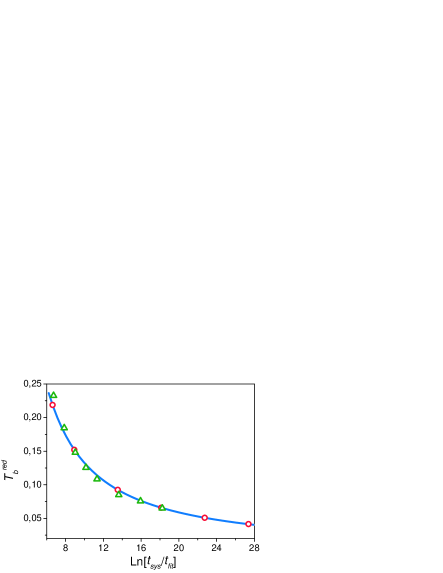
Figure 6: Dependences of $T_{b}^{\rm red}$ on the effective measuring time $t_{\rm{sys}}$ (the number of MC steps) for the MC method (triangles) and the RM (circles). The solid curve corresponds to the calculations by formulas (23) and (24)

time was obtained in the form

$$t_{\rm red}^{\rm{MC}}\approx nN_{\rm{MC}}/450.$$ (29)

One can estimate the number of MC steps which corresponds to the measuring time $t\nu_{0}=10^{10}$. It equals approximately $5\times 10^{12}$. Taking into account that one MC step contains a few tens of operations and that a modeling is performed for an ensemble of particles, the necessary computational resources exceed $10^{14}$ operations. Thus, it is concluded that the computational capability of modern computers is not sufficient to carry out the real time modeling. It is obvious that, for some calculations, it is more important to deal with a great number of particles in an ensemble and less important whether the number of MC steps is great or small. However, to simulate, for example, the ZFC/FC (zero field cooling/field cooling) procedure, the value of the measuring time is likely to be decisive.

Let us discuss the origin of the parameter $t_{\rm{fit}}$ for the MC procedure. The only parameter which we have not yet varied is the generation aperture $\Delta\theta$. It was noted that the MC calculations above were carried out under the condition that $\Delta\theta=6{{}^{\circ}}$. Let us start from the assumption that it is the parameter $\Delta\theta$ that determines the $t_{\rm{fit}}$ value. To make sure of this, we performed the MC calculations of $T_{b}^{\rm red}(N_{\rm{MC}})$ dependences for various values of aperture ($\Delta\theta=1.5\div 48{{}^{\circ}}$).

Figure 7: The $T_{b}^{\rm red}(nM_{\rm{MC}})$ dependences calculated by MC method for various values of aperture $\Delta\theta=1.5$, $3$, $6$, $12$, $24$, and $48^{\circ}$ (circles). Solid lines are the fitting of the obtained results with the function $T_{\rm{b-scan}}(nN_{\rm{MC}}/t_{\rm{fit}})$

Figure 7 presents the results of this modeling. As is seen from the figure, for the calculations with a small number of MC steps, $T_{b}^{\rm{red}}$ strongly depends on $N_{\rm{MC}}$. As $N_{\rm{MC}}$ increases, the aperture value to a lesser extent affects $T_{b}^{\rm red}$. At the same time, a family of $T_{b}^{\rm red}\left[\ln(nN_{\rm{MC}})\right]$ dependences can be well approximated by a function $T_{\rm{b-scan}}(nN_{\rm{MC}}/t_{\rm{fit}})$. It follows from general considerations that $t_{\rm{fit}}(\Delta\theta)$ should be dependent on $U_{r}$, its derivatives, or its integrals. However, we have not succeed in finding the precise analytic dependence. We can only note that, for $\Delta\theta<45{{}^{\circ}}$, the admissible expression resulted from the fitting of the data in Fig. 7 is

$$t_{\rm{fit}}\approx 4.9/\left[\sin^{2}(\Delta\theta)\right].$$ (30)

Thus, we have obtained the final expressions which answer a question about which measuring time corresponds to the MC calculations:

$$t_{\rm red}^{\rm{MC}}\approx\;{\frac{{\sin^{2}(\Delta\theta)}}{{4.9\;}}}nN_{\rm{MC}},$$ (31)

$$~{}T_{b}^{\rm{MC}}\approx T_{\rm{b-scan}}\left[n{\frac{{N_{\rm{MC}}}}{{4.9}}}\sin^{2}(\Delta\theta)\right].$$ (32)

VI Conclusions

In this work, the recursion method has been developed for the calculations of the magnetic properties of the ensemble of single-domain particles. Its applicability to the system of oriented particles with a uniaxial anisotropy is demonstrated. There are no hindrances to apply such a procedure to the case of a cubic anisotropy, introduce the distribution function for a certain parameter, make the anisotropy constant temperature-dependent, or even introduce the dipole-dipole interaction between the particles of an ensemble. It is also not difficult to model the ZFC/FC procedure. In our opinion, the RM results will far better reflect the real experiments, than the results of the MC modeling.

The relation, which correlates the magnetic parameters of the ensemble of uniaxially anisotropic magnetic particles with a measuring time for these properties in various experimental procedures, is obtained.

It is shown that, depending on a kind of experiment, the relationship between the blocking temperature and the measuring time has somewhat different forms.

The calculations of the magnetization curves for the ensemble of uniaxial single-domain particles are carried out for different measuring times. The similar calculations performed by the Monte-Carlo technique confirm the adequacy of the method developed here. The latter method requires far less  computational  resources

in comparison with the modeling of an analogous task by the Monte–Carlo method.

With the use of the new method, we succeeded in the establishment of the empirical dependence between the number of MC steps and the generation aperture of a random direction of the magnetic moment, on the one hand, and the measuring time, which corresponds to these parameters, on the other hand. It is shown that the parameters, which are usually used for the MC modeling of the behavior of ensembles of magnetic particles, correspond to unlikely short values of the measuring time.

Translated from Ukrainian by A.I. Tovstolytkin

[1] E.C. Stoner and E.P. Wohlfarth, Philos. Trans. Roy. Soc. London, Ser. A 240, 599 (1948).

[2] S.V. Vonsovskii, Magnetism (Moscow, Nauka, 1971), Chapter 23, Section 6 (in Russian).

[3] L. Neel, Ann. Geophys. 5, 99 (1949).

[4] W.F. Brown, Phys. Rev. 130, 1677 (1963).

[5] H. Pfeiffer, Phys. Status Solidi A 118, 295 (1990).

[6] Lin He and Chinping Chen, Phys. Rev. B 75, 184424 (2007).

[7] J. García-Otero, M. Porto, J. Rivas, and A. Bunde, J. Appl. Phys. 85, 2287 (1999).

[8] O. Iglesias, A. Labarta, Physica B 372, 247 (2005).

[9] O. Iglesias, A. Labarta, Phys. Rev. B 63, 184416 (2001).

[10]D.A. Dimitrov and G.M. Wysin, Phys. Rev. B 54, 9237 (1996).

[11] L. Wang, J. Ding, H.Z. Kong, Y. Li, and Y.P. Feng, Phys. Rev. B 64, 214410 (2001).

[12] O.V. Billoni, S.A. Cannas, and F.A. Tamarit, Phys. Rev. B 72, 104407 (2005).

[13] R.W. Chantrell, N. Walmsley, J. Gore, and M. Maylin, Phys. Rev. B 63, 024410 (2000).

[14] M.A. Chuev, Pis’ma v Zh. Eksp. Teor. Fiz. 85, 744 (2007).

[15] O. Michele, J. Hesse, and H. Bremers, J. Phys.: Cond. Matter 18, 4921 (2006).

[16] N. Metropolis, A.W. Rosenbluth, M.N. Rosenbluth, A.H. Teller, and E. Teller, J. Chem. Phys. 21, 1087 (1953).

[17] C.M.P. Russell and K.M. Unruh, J. Appl. Phys. 99, 08H909 (2006).

[18] R.M. Corless, G.H. Gonnet, D.E.J. Hare et al., Adv. Comput. Math. 5, 329 (1996).

[19] S.R. Valluri D.J. Jeffrey, and R.M. Corless, Canadian J. Phys. 78, 823 (2000).