Component models for large networks

Abstract

Being among the easiest ways to find meaningful structure from discrete data, Latent Dirichlet Allocation (LDA) and related component models have been applied widely. They are simple, computationally fast and scalable, interpretable, and admit nonparametric priors. In the currently popular field of network modeling, relatively little work has taken uncertainty of data seriously in the Bayesian sense, and component models have been introduced to the field only recently, by treating each node as a bag of out-going links. We introduce an alternative, interaction component model for communities (ICMc), where the whole network is a bag of links, stemming from different components. The former finds both disassortative and assortative structure, while the alternative assumes assortativity and finds community-like structures like the earlier methods motivated by physics. With Dirichlet Process priors and an efficient implementation the models are highly scalable, as demonstrated with a social network from the Last.fm web site, with 670,000 nodes and 1.89 million links.

Keywords: Latent-Component Mixture Model, Social Network, Probabilistic Community Finding, Nonparametric Bayesian

1 Introduction

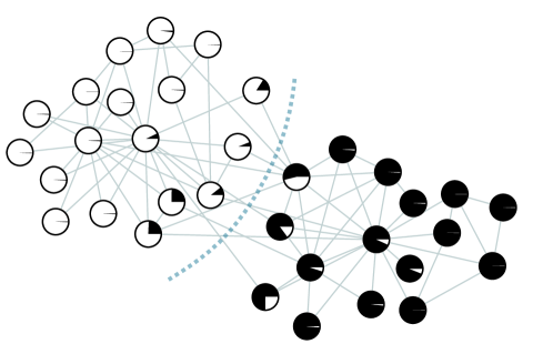
Figure 1: One of the models (ICMc) on a classic small network, the Karate club. Zachary (1977) observed the social interactions (edges) between 34 members of a karate club over two years. During this period, there was disagreement among the club members which eventually led to the splitting of the club (dashed line). Black and white depict the degree of component memberships obtained by the model, without knowing the correct split.

Data collections representable as networks, or sets of binary relations between vertices, appear now frequently in many fields, including social networks and interaction networks in biology (Fig. 1). Consequently, inferring properties of the network vertices from the edges has become a common data mining problem. Most of the work has been about dividing the vertices into relatively well-connected subsets, or communities (Fortunato and Castellano, 2007). Most papers on communities have been inspired by graph theory and physics, as is a large field of fundamental network-related work not directly relevant here. Especially optimizing a measure of good division called modularity (Newman, 2006) has gained success but is not without its problems (Fortunato and Barthelemy, 2007; Kumpula et al., 2007).

A feature and potential problem of modularity is that it takes the observed edges granted, while network data are typically not a complete description of reality but comes with errors, omissions and uncertainties. Some links may be spurious, for instance due to measurement noise in biological networks, and some potential links may be missing, for instance friendship links of newcomers in social networks. Probabilistic generative models are a tool for modeling and inference under such uncertainty. They treat the links as random events, and give an explicit structure for the observed data and its uncertainty. Compared to non-stochastic methods, they are therefore likely to perform well as long as their assumptions are valid: They may reveal properties of networks that are difficult to observe with non-statistical techniques from the noisy and incomplete data, and they also offer a groundwork for new conceptual developments. For example, it may be argued that network communities should be defined in terms of stochastic models that do not take links at face value but instead give them an underlying stochastic structure that should be realistic given an application. On the down side, probabilistic methods are not always scalable, and they may be difficult to understand, apply and trust by people from other fields, especially if the estimation process is complex.

Probabilistic models of network connectivity have been introduced recently. Mixtures of latent components (Newman and Leicht, 2006), analogous to finite mixture models for vectorial data, are attractive because of ease of interpretation, but the extensive numbers of parameters encumber straightforward fitting attempts. A very promising development called stochastic block models (Airodi et al., 2008—but also Daudin et al., 2007; Hofman and Wiggins, 2007) groups the nodes into blocks and explains the links in terms of homogeneous connections between pairs of groups. Finally, links can be explained by the proximity of nodes in a latent space created by a logistic link (Handcock et al., 2007). These models have been successively applied to various networks from sociology and biology, up to the size of thousands or tens of thousands of nodes. With heuristic improvements, stochastic block models are expected to scale up to over one million nodes (E. Airoldi, p.c.), but in general the computational bottleneck is scalability.

The models discussed in this paper are generative probabilistic models that decompose the links into components, but their structure makes them scalable to networks with at least $10^{3}\dots 10^{6}$ nodes, and up to thousands of latent components—as long as the networks are sparse enough. The Simple Social Network LDA (SSN-LDA) model presented by Zhang et al. (2007) is identical to the Latent Dirichlet Allocation (LDA; Buntine, 2002; Blei et al., 2003) model, originally applied to text collections. It is also a conceptual although not a geneologic successor of the mixture model by Newman and Leicht (2006). The SSN-LDA model assumes that each node is a bag of outgoing links, and models each outgoing set of links as a mixture over latent components. The components are the same for each node, but their proportions differ.

As an alternative we introduce a component model for relational data, where each link is directly assumed to come from a latent component, and the whole network is a bag of links (Sinkkonen et al., 2007). This model is particularly well suited for modeling of community-type structure in networks. For conciseness, we call it ICMc (interaction component model for communities), the latter ’c’ reminding of the fact that it is easy to generate new models from the family of ICMc and SSN-LDA, with slightly different generative assumptions and requirements for data.

Both ICMc and SSN-LDA represent a set of links as a probabilistic mixture over latent components. Depending on the prior, the models can find either a given number of latent components, or nonparametrically adjust the number of components to the data, guided by a diversity parameter. Moreover, depending on parameters, they are capable of finding either subnetworks or more graded, latent-space-like structures.

Both models can be easily and efficiently fitted to data by collapsed Gibbs sampling (Neal, 2000), an MCMC technique for sampling from the posterior where parameters have been integrated out and latent variables are sampled. In the component models the latent variables give the assigments of the links to the components. Critical for successful scaling to large networks is sparseness of representations; here the component assignments of the links, the variables that are sampled in the collapsed Gibbs, can be efficiently represented as sparse arrays, trees, and hash maps.

We compare the two models on two citation networks with a few thousand nodes, CiteSeer and Cora (Sen and Getoor, 2007), and demostrate their properties on smaller networks. As a demonstration of a larger-scale problem, musical tastes of people are derived from the friendship network of the online music service Last.fm (www.last.fm), with over 650,000 vertices vertices and almost two million edges.

SSN-LDA ICMc               SSN-LDA ICMc

             

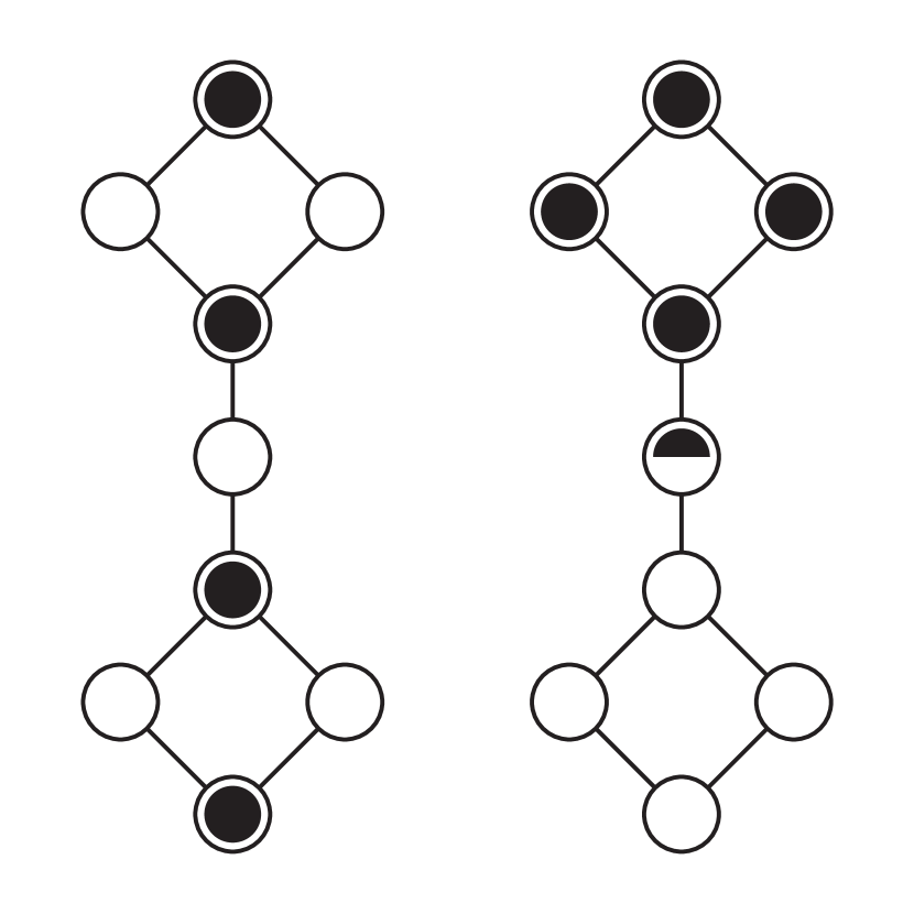
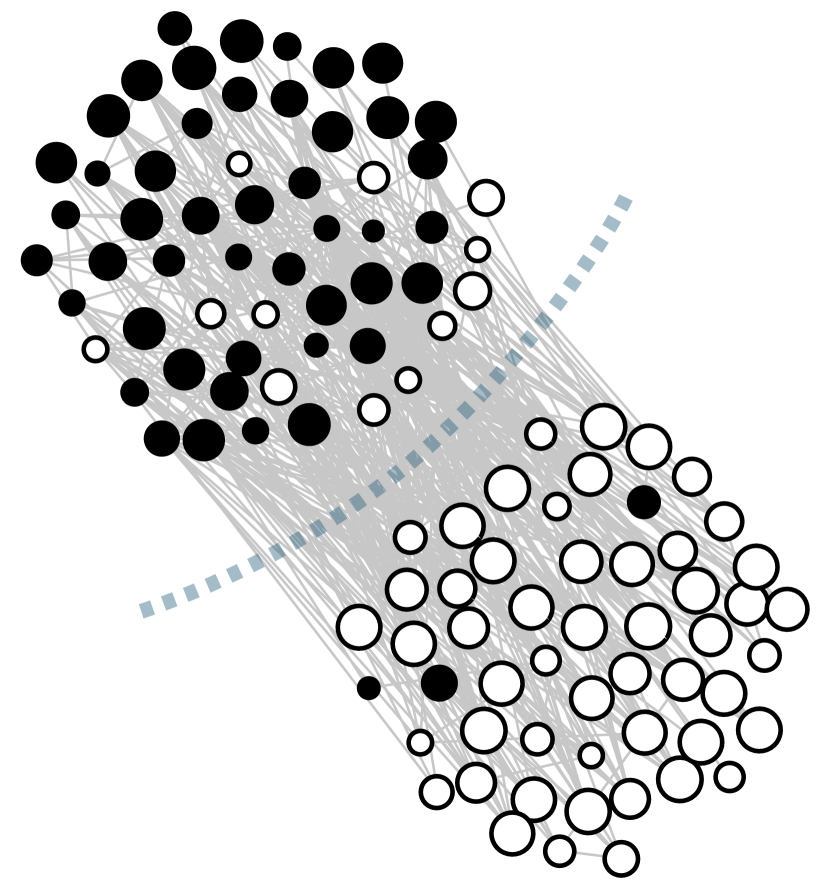
Figure 2: Network structure and component models. Left: A toy network split into two components (black and white). SSN-LDA produces both assortative and disassortative components, but here favors the disassortative interpretation, grouping nodes by common external connectivity. The ICMc solution is assortative and more community-like. Right: The Adj-Noun network of adjective and noun co-occurrences is bipartite, with a negative modularity of -0.241. SSN-LDA, not limited to assortative solutions, finds the underlying structure (node size represents certainty). Modularity of the SSN-LDA solution (black vs. white) is -0.262 and that of ICMc 0.188. See Table 1 for details of Adj-Noun.

2 Two scalable network models

SSN-LDA models directed links. A unique mixing pattern over latent link target profiles is associated to each node. (Technical details are presented later, e.g., in Fig. 4, right). The latent profiles correspond to topics of text document models, the original application of LDA. If the node memberships in latent profiles are sharp enough, that is, if the nodes are mainly associated to one profile only, the profiles can be interpreted as subgraphs. The grouping criterion is a probabilistic version of the structural equivalence principle of sociology (Michaelson and Contractor, 1992): Two nodes belong to the same group if their role in the network topology is similar, that is, they link to the same (other) nodes.

In ICMc, a unique mixture over latent components is associated with each node, and linking is unstructured inside a component. Instead of structural equivalence, the criterion for subgroups is homogeneous, symmetric internal connectivity. Link directions are therefore not modelled. A related social concept is subgroup cohesion (Wasserman and Faust, 1994), where latent similarity results in connections inside the group, instead of linking into some common third party. As a result, the network looks homophilic (Lazarsfeld and Merton, 1954); the connected nodes tend to be relatively similar by their non-network properties.

For technical reasons, the parameterization of linking within a component in ICMc is in terms of linking probabilities over the components; memberships of nodes in components can be obtained from these parameters by the Bayes rule. Equivalently, the model can be described as modeling the whole graph as a bag of links. Each link comes from a component specified by a latent variable $z$ (Fig. 4, left). Each component chooses the endpoints of a link from a component-specific (multinomial) distribution over the nodes, parameterized by $m_{z}$.

A further helpful distinction is that of assortative and disassortative network properties. A network is assortative with respect to a property if the property tends to co-occur in connected nodes more often than expected by change (Newman, 2003). The opposite, negative correlation in adjacent nodes, is called disassortativity. SSN-LDA can in principle find either kinds of structures, while ICMc tends to find only assortative structure. Modularity, a quality measure for community detection (Newman, 2006), can at least to a degree be used as a measure of assortativity; if it is negative for a partitioning of the network, the partitioning is disassortative (Fortunato and Castellano, 2007). Unfortunately, comparing modularities of partitionings over different networks is in general not justified (Fortunato and Castellano, 2007), and hence we cannot use it to compare the modeling problems.

One would expect ICMc to find communities from social and other networks better than the less specialized SSN-LDA, as long as linking results from homophily and the communities can be assumed assortative. The reason is that a model having less degrees of freedom in its parameterization will be able to more accurately estimate the parameters from the relatively small observed data sets. On the other hand, ICMc should be unable to find disassortative structures. This seems to indeed hold in some extreme cases (Fig. 2), but in practice differences are often graded and harder to attribute to properties of the network (Fig. 3).

The behavior of both SSN-LDA and ICMc are determined by their hyperparameters. Both models can be made to prefer either latent components of equal size, or to allow heavy size variation. Even more importantly, either graded or non-overlapping components can be preferred. In graded components the community membership probabilities are akin to coordinates in a latent space, while non-overlapping components divide the nodes sharply into clusters.

Both models can accommodate integer link weights in the sense of generating multiple links between two nodes. On the other hand, the models work particularly efficiently for sparse binary links: If data is sparse, link probabilties are small overall, multiple links even more improbable, and the model effectively generates binary data.

The SSN-LDA model is originally based on a finite mixture (Zhang et al., 2007), but it is easily extended for a Dirichlet process prior (DP prior; Blackwell and MacQueen, 1973; Neal, 2000), while ICMc is originally with a DP prior (Sinkkonen et al., 2007), but here applied also in its finite form.

The models are demonstrated on three small networks in Figures 1 and 3. The first is the Karate network originating from a study by Zachary (1977). In the study Zachary observed the social interactions between 34 members of a karate club over two years. During this period, there was disagreement among the club members which led to the splitting of the club. Figure 1 demonstrates that ICMc finds the splitting.

The second demonstration network is the Football network (Girvan and Newman, 2002), which depicts American football games between Division IA colleges during the fall season 2000. The nodes of the network represent football teams and edges the games between the teams. There is a known community structure for the network in the form of conferences. In general, games between teams that belong to the same conference are more frequent than games between teams that belong to different conferences, but sometimes teams prefer to play mostly against teams in other conferences. Both models find the structure as seen in Figure 3, SSN-LDA slightly more accurately. ICMc is somewhat more accurate on another network derived from political blogs.

Table 1: Network characteristics and modeling parameters for the small and medium-size networks. In the table, $I$ is the number of nodes in the network, $L$ is the number of edges, $Q$ the ground cluster modularity, and $\alpha_{\mathit{Dir}}$ and $\beta$ are the hyperparameters of the models.

				ICMc		SSN-LDA
Network	$I$	$L$	$Q$	$\alpha_{\mathit{Dir}}$	$\beta$	$\alpha_{\mathit{Dir}}$	$\beta$
Adj-Noun	112	423	-0.241	0.5	0.2	0.5	0.2
Football	115	613	0.554	0.083	0.03	0.083	0.7
Polblogs	1 222	16 714	0.410	0.5	0.003	0.5	0.4
Citeseer	2 120	3 678	0.517	0.166	0.04	0.166	0.006
Cora	2 485	5 067	0.630	0.143	0.02	0.143	0.025

ICMc SSN-LDA

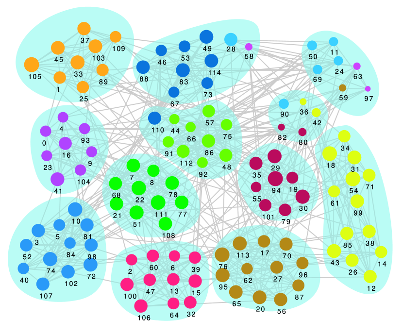
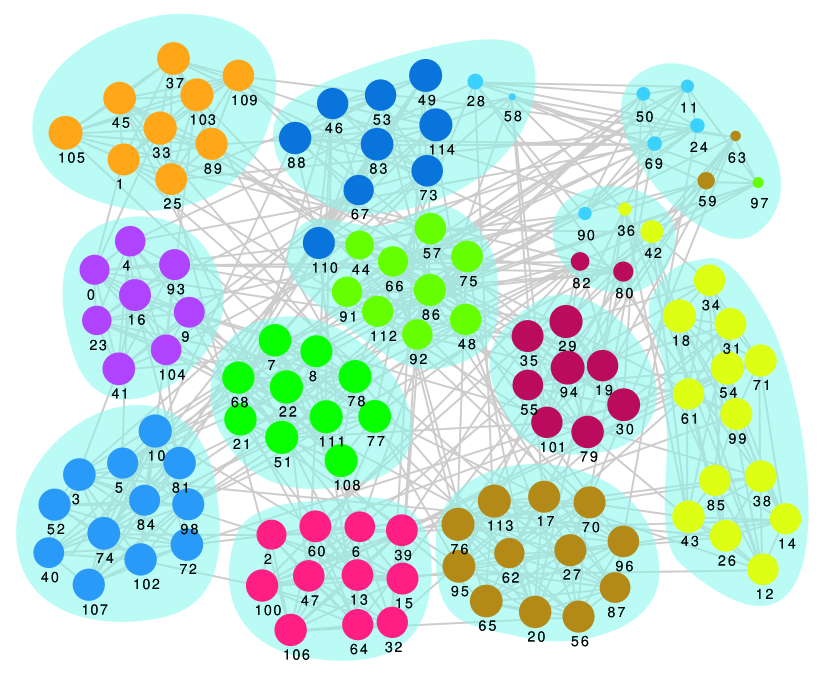
Figure 3: Relative performance of ICMc and SSN-LDA varies for different networks. Above: ICMc performs better for a network of political blogs, as measured by the perplexity of the components, while SSN-LDA is better for a network of US football games. Reasons for the differences are unclear, although they might be related to the assortativity of the networks with respect to the ground clusters (political orientation and football conferences). Below: Despite perplexity differences, the solutions are qualitatively very similar. For the Football network, main differences are in the certainty of cluster assignments. Shaded areas show the borders of the conferences, while community assignments by the model and their certainty are depicted by node color and size, respectively. See Table 1 for details of the networks and model parameters.

2.1 Interaction Component Model for Communities (ICMc)

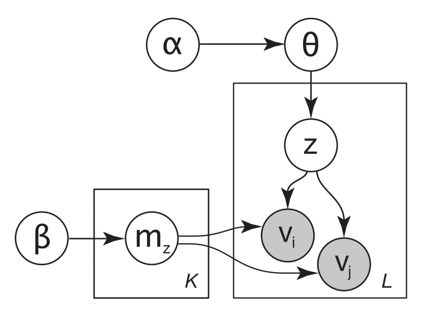
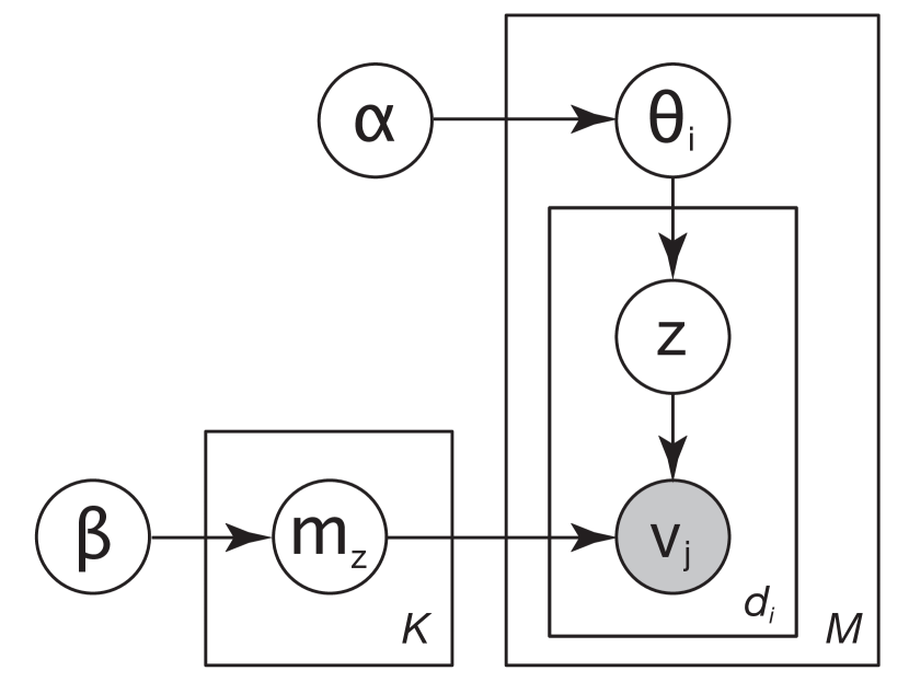
Figure 4: The ICMc model (left) and SSN-LDA (right). SSN-LDA is effectively the Latent Dirichlet Allocation (LDA; Buntine, 2002; Blei et al., 2003) applied to network data, with nodes playing both the role of ’words’, at the receiving end of links, and ’documents’ at the sending end. ICMc has no hierarchy level for nodes. Instead, it generates two nodes for each link; the links are undirected. See Section 2 for the notation and further discussion.

The generative process out of which the network is supposed to arise is the following (see Fig. 4 for a diagram); it is parameterized by the hyperparameters $(\alpha,\beta)$.

• Generate a multinomial distribution $\theta$ over latent components $z$. For $K$ components, the multinomial is generated from a $K$-dimensional Dirichlet distribution with all parameters set to $\alpha_{\mathit{Dir}}$, $\mathop{\mathrm{Dir}}_{\mathrm{sym}}^{K}(\alpha_{\mathit{Dir}})$, and for an infinite number of components from the Dirichlet process $\mathop{\mathrm{DP}}(\alpha_{\mathit{DP}})$.

• To each $z$, associate a multinomial distribution over the $M$ vertices $i$ by sampling the multinomial parameters $m_{z}$ from the Dirichlet distribution $\mathop{\mathrm{Dir}}_{\mathrm{sym}}^{M}(\beta)$. (To clarify, we have $\sum_{i}m_{zi}=1$ for each $z$, and $\sum_{z}\theta_{z}=1\,$.);

• Then repeat for each link $l=1\dots L$:

  • Draw a latent component $z$ from the multinomial $\theta$.

  • Choose two nodes, $i$ and $j$, independently of each other, with probabilities $m_{z}$; set up a nondirectional link between $i$ and $j$.

Within components, edges are generated independently of each other; the non-random structure of the network emerges from the tendency of components to prefer certain vertices (that is, $m$). In contrast to many other network models, the latent variables operate on the edge level, not on the vertex level. There is no explicit hierarchy level for vertices, but because vertices typically have several edges, they are implicitly treated as mixtures over the latent components. Finally, the model is parameterized to generate self-links and multi-edges because this choice allows sparse implementations which would not be directly possible with a potential alternative model that would generate binary links from the Bernoulli distribution.

Although in the case of a Dirichlet process prior the number of potentially generated components is infinite, the prior gives an uneven distribution over the components. Therefore, with a suitably small value of $\alpha_{\mathit{DP}}$, we observe much fewer components than the number of links is, and the model is useful. On the other hand, $\beta$ describes the unevenness of the degree distribution of the nodes within components: a high $\beta$ tends to give components spanning over all nodes, while a small $\beta$ prefers mutually exclusive, community-like components.

We have estimated the model with Gibbs sampling (Geman and Geman, 1984), a variant of MCMC methods that produce samples from the posterior distribution of the model parameters and the latent component memberships. As a side note, maximum likelihood or MAP estimation of the model is not sensible since the number of parameters and latent variables is large compared with the available data, It is easy to derive an EM algorithm for the finite-mixture ICMc, but it gets stuck into suboptimal local posterior maximums at the borders of the parameter space.

We use Gibbs sampling with some of the model parameters integrated out, called Rao-Blackwellized, or collapsed (Neal, 2000). (For the joint distribution of the model and the derivation of the estimation algorithm see the Appendix). In the collapsed Gibbs estimation algorithm the unknown model parameters $m_{zi}$ and $\theta_{z}$ are marginalized away and only the latent classes of the edges, $z_{l}$, are sampled, one edge at a time. In general, we denote edge counts per component by $n_{z}$, component-wise vertex degrees by $k_{zi}$, and the endpoints of the left-out edge by $(i,j)$. Then delete one edge, resulting in counts $(n^{\prime},k^{\prime},N^{\prime})$ that are equal to $(n,k,N)$ but without the one edge. The component probabilities of the left-out edge are

$$p(z|i,j)\propto\frac{k^{\prime}_{zi}+\beta}{2n^{\prime}_{z}+1+M\beta}\times\frac{k^{\prime}_{zj}+\beta}{2n^{\prime}_{z}+M\beta}\times\frac{n^{\prime}_{z}+\alpha_{\mathit{Dir}}}{N^{\prime}+K\alpha_{\mathit{Dir}}}$$ (1)

for the Dirichlet prior, and

$$p(z|i,j)\propto\frac{k^{\prime}_{zi}+\beta}{2n^{\prime}_{z}+1+M\beta}\times\frac{k^{\prime}_{zj}+\beta}{2n^{\prime}_{z}+M\beta}\times\frac{\mathrm{C}(n^{\prime}_{z},\alpha_{\mathit{DP}})}{N^{\prime}+\alpha_{\mathit{DP}}}$$ (2)

for the Dirichlet process prior. The ’chooser’ function $\mathrm{C}(n_{z},\alpha_{\mathit{DP}})\equiv n_{z}$ if $n_{z}\neq 0$ and $\mathrm{C}(0,\alpha_{\mathit{DP}})=\alpha_{\mathit{DP}}$. The case with $\alpha_{\mathit{DP}}$, as opposed to $n_{z}$, corresponds to a new component with no other links so far.

This sampling step is simply repeated iteratively for all links, until convergence to the posterior distribution, or until the results are satisfactory by some other measure. A particularly elegant, although not necessarily the most efficient initialization of the sampler starts from empty urns, with $k_{zi}=n_{z}=N=0$, then runs through the edges once in a random order and populates the urns according to (1) or (2) while counting only the edges seen so far.

Algorithm 1 ICMc-Gibbs.   A simple implementation for the ICMc algoritm with a Dirichlet prior.

• $\textnormal{Simple-Gibbs-Sampling}(\alpha_{\mathit{Dir}},\beta,L)$
     $t_{nodes}\leftarrow$ node count for $c\leftarrow 1$ to $\mathop{\mathit{components}}\nolimits$ do$\rhd$ initialize data structures $A[c]\leftarrow 0$ for $n\leftarrow 1$ to $t_{nodes}$ do$\;K[n,c]\leftarrow 0$ for $i\leftarrow 1$ to $\mathop{\mathit{iterations}}\nolimits$ do$\rhd$ main iteration loop foreach $l$ in $L$ do $v_{i},v_{j}\leftarrow$ first and second node of $l$ if ${i\neq 1}$ do $z_{old}\leftarrow Z[l]$ decrement $K[v_{i},z_{old}],K[v_{j},z_{old}],A[z_{old}]$ for $c\leftarrow 1$ to $\mathop{\mathit{components}}\nolimits$ do $P[c]\leftarrow\textnormal{Calc-Probability}(A[c],K[v_{i},c],K[v_{j},c],t_{nodes},\alpha_{\mathit{Dir}},\beta)$ $z_{new}\leftarrow$ sample index from $P$ $Z[l]\leftarrow z_{new}$ increment $K[v_{i},z_{new}],K[v_{j},z_{new}],A[z_{new}]$ return K, Z

• $\textnormal{Calc-Probability}(n_{c},k_{a},k_{b},t_{nodes},\alpha_{\mathit{Dir}},\beta)$
     return $\dfrac{(k_{a}+\beta)(k_{b}+\beta)(n_{c}+\alpha_{\mathit{Dir}})}{(2n_{c}+1+\beta t_{nodes})(2n_{c}+\beta t_{nodes})}$

The goal of model fitting is usually to infer community memberships of the nodes. From the Bayes rule we obtain

$$p(z|i)=\frac{\theta_{z}m_{zi}}{\sum_{z^{\prime}}\theta_{z^{\prime}}m_{z^{\prime}i}}\;.$$ (3)

A sample of the marginalized parameters $\theta$ and $m$ can be reconstructed from each realization of the counts $(k,n)$ by sampling from the conditional Dirichlet distributions given the priors and the counts:

$$\theta\sim\mathop{\mathrm{Dir}}_{z}(n_{z}+\alpha_{\mathit{Dir}})\,\,\,\mathrm{or}\,\,\,\theta\sim\mathop{\mathrm{Dir}}_{z}(\left\{n_{z},\alpha_{\mathit{DP}}\right\}_{z})\,,\,\,\,\mathrm{and}\,\,\,m_{z}\sim\mathop{\mathrm{Dir}}_{i}(k_{zi}+\beta)\;.$$ (4)

Note that $n_{z}=\sum_{i}k_{zi}/2$. In the case of the Dirichlet process prior, the parameter $\theta$ has probabilities of the components with at least one assigned link, and then the probability of all empty components summed up into the last bin. These correspond to the Dirichlet parameters $n$ and $\alpha_{\mathit{DP}}$, respectively.

Even if one wants to reconstruct $\theta$ and $m$, collapsed Gibbs is likely to be faster than full Gibbs. The reasons are twofold: Firstly, Gibbs converges faster when the parameter updates are not in the main loop. Secondly, one usually uses decimation in sampling from the converged chain, and the $(\theta,m)$ need to be constructed only for the decimated samples.

It is often sufficient to estimate the community memberships from the expected values of the marginalized parameters,

$$\hat{\theta}=\frac{n_{z}+\alpha_{\mathit{Dir}}}{\sum_{z^{\prime}}n_{z^{\prime}}+K\alpha_{\mathit{Dir}}}\,\,\,\mathrm{or}\,\,\,\hat{\theta}=\frac{n_{z}}{\sum_{z^{\prime}}n_{z^{\prime}}+\alpha_{\mathit{DP}}}\;,$$ (5)

and

$$\hat{m}_{z}=\frac{k_{zi}+\beta}{\sum_{i^{\prime}}k_{zi^{\prime}}+M\beta}\;.$$ (6)

Substituting the expectations into (3), we find that for small $\alpha$ and $\beta$,

$$p(z|i)\approx\frac{k_{zi}}{\sum_{z^{\prime}}k_{z^{\prime}i}}$$ (7)

is a good approximation.

Prediction for new data is straightforward; the component memberships of the links associated to a new node can be sampled from (1), given old links. If the new links are not conditionally independent given the old data, one can run a short Gibbs iteration on the new links.

2.2 SSN-LDA

SSN-LDA (Zhang et al., 2007) also has two hyperparameters, denoted by $\alpha$ and $\beta$, but they are in a slightly different role than in ICMc (see Fig. 4). The generative process is as follows:

• Generate $M$ multinomial distributions $\theta_{i}$, $i=1,\dots,M$, over latent components $z$, $z=1,\dots,K$, either from a $K$-dimensional Dirichlet distribution $\mathop{\mathrm{Dir}}_{\mathrm{sym}}^{K}(\alpha_{\mathit{Dir}})$, or from the Dirichlet process $\mathop{\mathrm{DP}}(\alpha_{\mathit{DP}})$.

• Assign a multinomial distribution $m_{z}$ over the vertices $i$ to each component $z$ by sampling from the Dirichlet distribution $\mathop{\mathrm{Dir}}_{\mathrm{sym}}^{M}(\beta)$.

• Then repeat for each link $l=1,\dots,L$, with sending nodes $i=1,\dots,M$:

  • Draw a latent component $z$ from the multinomial $\theta_{i}$.

  • Choose the link endpoint $j$ with probabilities $m_{z}$; set up a directional link between $i$ and $j$.

We have presented the generative process of links in a flat form to make comparison to ICMc easier; in step 2, the loop over nodes is avoided by referring to the node indices $i$ associated to links.

In contrast to ICMc, SSN-LDA has the node as an explicit hierarchy level—in the generative model, there are the parameters $\theta$ for each node separately, and $\alpha$ is the common hyperparameter of these node-wise distributions. As in ICMc, the hyperparameters $m$ are associated to latent components over nodes, and $\beta$ determines their prior. But now $m$ determines only the probabilities of the receiving nodes. Sending probabilities, associated to starting points $i$ of the links, are modeled by $\theta$.

Collapsed Gibbs sampling operates on two sets of counts: $n_{iz}$ that counts the sender–component combinations $(i,z)$ for links, originating from step (2.1) of the generative process, and $k_{zj}$ counting the receiver–component combinations $(j,z)$ from step (2.2) of the process. Following Griffiths and Steyvers (2004), and Zhang et al. (2007), the conditional probabilities for sampling a left-out link in a collapsed Gibbs iteration, given hyperparameters and all other links, is

$$p(z|i,j)\propto\frac{k^{\prime}_{zj}+\beta}{k^{\prime}_{z\cdot}+M\beta}\times\frac{n^{\prime}_{iz}+\alpha_{\mathit{Dir}}}{n^{\prime}_{i\cdot}+K\alpha_{\mathit{Dir}}}\;,$$ (8)

where sums over counts $k^{\prime}$ and $n^{\prime}$ have been denoted by the dot notation. We have omitted the derivation of the Dirichlet process variant, because it is very similar to the derivation of the DP ICMc (see the Appendix), leading to:

$$p(z|i,j)\propto\frac{k^{\prime}_{zj}+\beta}{k^{\prime}_{z\cdot}+M\beta}\times\frac{\mathrm{C}(n^{\prime}_{iz},\alpha_{\mathit{DP}})}{n^{\prime}_{i\cdot}}\;.$$ (9)

Again, parameter reconstruction for $\theta$ and $m$ can be done either by sampling from the corresponding Dirichlet distributions, or by computing the conditional MAP estimates, either roughly or exactly including priors. As with ICMc, we have used the rough alternative suitable for small values of $\alpha$ and $\beta$:

$$p(z|i)\approx\frac{n_{iz}}{n_{i\cdot}}\;.$$ (10)

This is for the community memberships of nodes as senders of links. Because in SSN-LDA links are directed, it is possible to define the memberships also in terms of received links,

$$p(z|j)\approx\frac{k_{zj}}{k_{\cdot j}}\;.$$ (11)

2.3 Efficient implementation of the collapsed Gibbs samplers

Large real-life networks are sparse almost by definition, and for efficiency it is important to preserve the sparseness in model structures. ICMc and SSN-LDA facilitate sparse structures, since likelihoods decompose into sums over existing links, and terms related to non-links do not appear.

Collapsed Gibbs sampling of ICMc and SSN-LDA needs tables for $n$ and $k$ which together, as a first approximation, are of the size complexity $O(MK)$. In addition one needs to keep track of the component identities of the links, an array of size $O(L)$. But in both models the degree of a node poses an upper limit for its component heterogeneity, so that only a few of the counts $k$, or $k$ and $n$ in LDA, are simultaneously non-zero, allowing sparse representation of the count tables. Therefore with hash tables memory consumption can be reduced to $O(M\bar{d}+L+K)$ where $\bar{d}$ is the average degree of a node. Because $\bar{d}=L/M$, memory consumption scales as $O(L+K)$.

Marginal sums of the count tables, notably $n$ in ICMc, can be represented in a sparse form and updated efficiently during sampling with the aid of a self-balancing binary tree. The idea of using a tree in sampling of discrete distributions was originally proposed by Wong and Easton (1980), and another method for using binary trees in simulations is provided by Blue et al. (1995). In our implementation the Arne-Andersson tree (AA tree) is used (see, e.g., Weiss, 1998), but other self-balancing binary trees would be equivalent in performance. A partial sum tree is formed, where in each node, the total probability of the node is stored, together with the sums of probabilities of both the left and right children of the node. When the probability of a node is changed, the modifications are propagated up to the parents of the node. Sampling proceeds recursively down the tree as a sequence of weighted Bernoulli samples.

These sparse representations, and the binary tree for the marginal sums, make it possible to run models with at least tens of thousands of components in an ordinary PC or server. These structures also fit well with the dynamic component numbers due to the Dirichlet process prior. With the data structures described above, running time per one Gibbs iteration over all the nodes becomes $O(L\,\bar{d}\;\log K)$. That is, the time needed for an iteration scales linearly in the number of edges and logarithmically in the number of components.

It is hard to give any general rule on the number of Gibbs iterations needed for convergence. Because the variables in the collapsed Gibbs algorithm correspond to links, the dependency graph of the variables is like the original network, but with the nodes being in the role of links, and vice versa. The path lenghts of the dependency network are therefore proportional to the path lengths of the original network. Let us assume that the average path length scales as $l\propto\log M$, as is the case with many small-world networks (Albert and Barabasi, 2002). In Gibbs, information diffusion over the network can be expected to take $l^{2}$ iterations, analogously to ordinary diffusion. This leads to the conjecture that the number of Gibbs iterations should be proportional to $\log^{2}M$.

3 Tests

We compared SSN-LDA and ICMc on two medium-scale social network datasets, Cora and Citeseer (Sen and Getoor, 2007), in the task of finding a predefined set of known clusters. Performance on large networks of $10^{5}\dots 10^{6}$ nodes is then demonstrated for one of the models (ICMc) with two friendship networks from the music site Last.fm.

3.1 ICMc vs. SSN-LDA

The Cora and the CiteSeer datasets consist of content descriptions of scientific publications and citations between them. The Cora dataset has 2,708 papers in seven predefined classes, while the CiteSeer dataset contains 3,312 publications in six classes. We used only the citation information, and the predefined classes as a ground truth for clustering. Nodes (publications) not belonging to the main components of the network were removed, and directional links were symmetrized. The resulting network for Cora has 2,120 nodes and for Citeseer 2,485 nodes (Table 1).

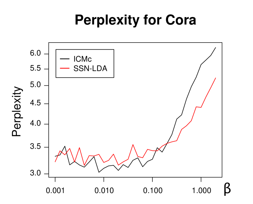
Figure 5: Gibbs samplers on the Cora citation set: convergence and sensitivity to the hyperparameter $\beta$. Left: Leave-one-out logarithmic posterior probability of the data for a single ICMc chain. This can be recorded easily during sampling as log probabilities of the drawn link assignments. We ran 50,000 iterations over the data, but about 15,000 would have been enough for convergence, and about 3,000 for getting useful results. SSN-LDA convergence was very similar. Right: Perplexity for the Cora dataset with a range of hyperparameter values $\beta$. Each reported value is an average of four chains. Both models are quite robust with respect to $\beta$.

Following Zhang et al. (2007) and our own experiences (Aukia, 2007), we fixed $\alpha_{\mathit{Dir}}=1/K$ for both models and datasets. Values for the parameter $\beta$ were chosen with pretests (Table 1 and Fig. 5). In general, the models with a Dirichlet prior and a small number of components are quite insensitive to values of $\alpha_{\mathit{Dir}}$ and $\beta$ within the range $0.001\dots 0.1$.

The Gibbs sampler was initialized as suggested in Section 2.3 and run for 50,000 iterations (see Fig. 5). We then took 100 samples at intervals of 100. Each sample consists of the latent cluster memberships $z$ for all links. Node memberships were constructed by (7) and (10) for each sample separately, and these were summed up to get confusion matrices.

Over the computed 50 chains, there is a good average correspondence between the found clusters and the original manual clustering of the data sets (Fig. 6). In terms of perplexity ICMc is able to recover the orignal clusters better than SSN-LDA, although the average confusion matrices are relatively similar. Results vary from chain to chain more than with small networks, indicating multiple local minima for the Gibbs sampler to get trapped into. (See Section 4 below for discussion on this behaviour.)

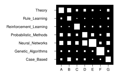
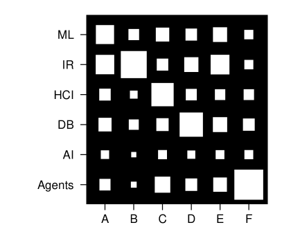
Figure 6: The models ICMc and SSN-LDA on two citation networks, Cora and CiteSeer. Above: Performance in finding true clusters, as measured by the perplexity of predicting ground-truth groups with the clusters. The average and 95% confidence intervals for the mean are over 50 chains. Below: Average confusion matrices between the found clusters (columns) and the true clusters (rows).

3.2 ICMc on Last.fm friendship network

Last.fm is an Internet site that learns the musical taste of its members on the basis of examples, and then constructs a personalized, radio-like music feed. The web site also has a richer array of services, including a possibility to announce friendships with other users. The friendships are initiated by a single party but are later mutual, forming a network with undirected links. Because friends tend to be similar, communities in the network would be relatively homogeneous by their musical taste and other characteristics. We use this similarity within communities to demostrate ICMc components.

Table 2: Last.fm networks and modeling parameters: $I$ is the number of nodes in the network, $L$ is the number of edges, and $\alpha_{\mathit{DP}}$ and $\beta$ are the hyperparameters.

			ICMc (DP)
Network	$I$	$L$	$\alpha_{\mathit{DP}}$	$\beta$
Full Last.fm	675 682	1 898 960	0.3	0.3
Last.fm USA	147 610	352 987	0.2	0.2

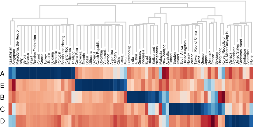
Figure 7: ICMc components (rows) of the Last.fm friendship network correlated with nationalities of the participants (columns). The full Last.fm network, about 675,000 nodes, was analyzed with the DP-version of ICMc. After a burn-in period of 19,000 iterations, 20 samples were taken at intervals of 50 iterations to get component memberships for the nodes. The running time was 16.4 hours when run in a single thread on an eight-core 2 GHz Intel Xeon. Dark blue and dark red denote the extremes of high and low co-occurrence counts, respectively. The columns are ordered and the tree produced by heatmap of the statistical environment R.

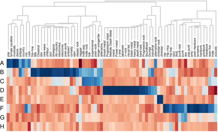
Figure 8: ICMc components (rows) of the Last.fm USA friendship network correlated with musical taste of the participants (columns). The model had the DP prior and was computed with a burn-in of 49,000 iterations, after which 20 samples were recorded at intervals of 50 iterations. The running time was 8.4 hours when run in a single thread on an eight-core 2 GHz Intel Xeon. Columns correspond to the most common tags given to the songs by the users themselves. Other details are as in Fig. 7.

The global Last.fm network had about 675,000 nodes and 1,9 million links, while the subset of US members had about 147,000 nodes and 353,000 links (Table 2). In addition to the friendships, we also crawled the nationalities of the site members in the network, as well as the tags they had associated to the music they like. The most common tags represent musical genres or subgenres, allowing interpretation of the components found from the network.

We modeled the networks with the ICMc, with its Dirichlet process prior adjusted to favor few components. (With different hyperparameters, it would have been possible to obtain thousands of local communities, but the interpretation of such a solution here to get an idea about its quality would be difficult.) See Table 2 and Figs. 7 and 8 for details and results.

The component structure of the full Last.fm network is primarily about geography or nationalities (Fig. 7). This was unexpected at first sight, but in hindsight it is not at all surprising, for people tend to bond mostly within their country or city, and the friendships in Last.fm are likely to reflect the relationships of the real world. Even if they did not, nationality would affect bonding. We also correlated the global component structure to musical taste, and while there are meaningful groups of genres (not shown, but see Fig. 8), it is hard to say which part of them arises due to the geographical division.

Although a more complex model would be needed to find both musical and geographical structure, the results show that ICMc is able to find homophilic structures from large networks. To get a better grasp of the musical homophily of the network, we also ran ICMc on a geographically more homogeneous subset of members who have announced to be from the US. This revealed a clear structure in terms of music preferences, as shown in Figure 8 and in Table 3. The model was able to separate light pop, more experimental music, “alternative,” metal, Christian, and a punk–hip-hop continuum. In addition, there were two components that are harder to interpret.

Cluster A
juggalo	$1.36$
pop	$1.34$
musicals	$1.32$
Sludge	${\color[rgb]{1,0,0}-1.89}$
black metal	${\color[rgb]{1,0,0}-1.98}$

Cluster B
shoegaze	$1.35$
Alt-country	$1.24$
post-punk	$1.22$
screamo	${\color[rgb]{1,0,0}-1.79}$
pop punk	${\color[rgb]{1,0,0}-3.16}$

Cluster C
indie	$0.46$
post-rock	$0.30$
folk	$0.22$
visual kei	${\color[rgb]{1,0,0}-1.86}$
j-pop	${\color[rgb]{1,0,0}-2.08}$

Cluster D
j-pop	$1.69$
visual kei	$1.68$
black metal	$1.56$
post-punk	${\color[rgb]{1,0,0}-1.21}$
psychedelic	${\color[rgb]{1,0,0}-1.41}$

Cluster E
christian	$1.53$
podcast	$1.01$
trance	$0.87$
shoegaze	${\color[rgb]{1,0,0}-1.54}$
Sludge	${\color[rgb]{1,0,0}-1.68}$

Cluster F
rnb	$1.33$
screamo	$1.21$
pop punk	$1.15$
Korean	${\color[rgb]{1,0,0}-2.25}$
psytrance	${\color[rgb]{1,0,0}-2.48}$

Cluster G
Jam	$1.35$
ska	$0.89$
hardcore	$0.47$
visual kei	${\color[rgb]{1,0,0}-1.43}$
j-pop	${\color[rgb]{1,0,0}-2.28}$

Cluster H
latin	$1.13$
chinese	$1.05$
psytrance	$0.70$
synthpop	${\color[rgb]{1,0,0}-1.54}$
juggalo	${\color[rgb]{1,0,0}-1.62}$

Table 3: The most likely and unlikely tags for each of the ICMc components in the Last.fm US network. The tables have been obtained by comparing the frequency of the tag to that expected in terms of its marginal probabilities. The table includes only tags for which the deviation from the expectation was reliable in terms of a binomial test (p=0.05). The numerical values are log-odds.

4 Discussion

We have presented two generative models for networks, of which ICMc is novel, and demonstrated and tested them on data sets of various sizes. Performance differences between the models were small; ICMc performed slightly better on networks with strong subgroup cohesion, while SSN-LDA had an edge in finding more disassortative network structures. If one is after communities in a social network, there are both theoretical and empirical reasons to prefer ICMc. The models do not have significant differences in implementation complexity or ease of use.

SSN-LDA can be seen as a further development of similar kinds of models earlier applied to text documents. On the other hand, it is also a generalization of the model by Newman and Leicht (2006), which interestingly shares notable similarity with earlier text document models (Hofmann, 2001). ICMc belongs to the same model family with LDA, but introduces a generative process that is more faithful to the idea of subgroup cohesion. An earlier formulation of subgroup cohesion is modularity (Newman and Girvan, 2004; Newman, 2006), for which ICMc or its likelihood could be seen as an alternative. It would be interesting to explore the relationship between these two, especially as our simulations show that in general modularity increases monotonically during a Gibbs run or saturates and only slightly decreases before convergence (Aukia, 2007).

Most of our tests were on networks with a known community structure, which allowed us to set the number of components in advance and use the Dirichlet prior. In preliminary tests we also tried Dirichlet process priors with these networks, but performance was naturally worse since they did not have the prior knowledge about the expected (“known”) component number. Another reason for the worse performance of DPs probably is that the size distribution of the communities is artificially even, for two related reasons. First, the networks have survived the selection process of becoming de factor standards for model testing. Second, in many cases the communities have been manually set up to make them maximally informative or otherwise handy. A small number of even-sized communities does not fit well with the Dirichlet process prior, which assumes either a small number of communities with rather unequal size, or a very large number with more equal size. It is likely that in real applications to social and biological networks the Dirichlet process performs relatively much better, because real-life communities tends to be of heterogenerous sizes.

The generative processes of simple models as discussed here are not meant to be realistic, at least not on higher hierarchical levels beyond the distributions generating the observed data. Instead, the ultimate criterion for generative processes should be empirical. Some abstract information about the networks can be coded to the generative processes, however. One obvious example is the assortative vs. disassortative nature of the network structure. It seems that getting this wrong is not catastrophical, but certainly using the right model improves performance. Another interesting detail are the Dirichlet priors. From their urn representations, it is obvious that they mimic the preferential attachment model of network generation (Albert and Barabasi, 2002) which produces relatively realistic degree distributions for social networks.

Even with the Dirichlet process prior one needs to choose the hyperparameters. Fortunately, the models seem to be quite robust in terms of the parameter $\beta$, and also in terms of $\alpha_{\mathit{Dir}}$ with the Dirichlet prior. It is possible to take $\beta$ into the sampling process as an MCMC step, because the marginal likelihood for $\beta$ is easy to compute. With the Dirichlet process prior, the parameter $\alpha_{\mathit{DP}}$ fundamentally affects the latent component diversity and therefore model complexity. For $\alpha$ one can use the proposed approximations of evidence, such as the harmonic mean estimator (Griffiths and Steyvers, 2004; Buntine and Jakulin, 2004)—it is known to be unstable but at least sometimes repairable (Raftery et al., 2007). Cross validation on the link level is still another possibility.

Although Gibbs sampling has a reputation of being slow compared to variational methods, a lot depends on how the slowness is measured. With topic models for texts, Gibbs is know to produce better results than variational LDA, at the cost of maybe 4–8 times the running time to convergence (Wray Buntine, p.c.). But according to Griffiths and Steyvers (2004), Fig. 1, collapsed Gibbs is actually faster, measured in floating point operations per second to attain a certain level of perplexity. The difference may partly be explained by implementational details, but one should also note that performance measurements should be relative to the goal: While in statistical inference convergence is essential, in predictive tasks the predictive performance counts, and often in practice a model is better if it gives better performance in a shorter running time, regardless of whether it has converged or not.

In fact, the whole notion of posterior convergence is problematic in models like LDA and ICMc with a high number of data, parameters and components. We do know that permutation modes exist and that the current Gibbs samplers fortunately find only one of them—if they found more, we would have a label switching problem. Even within a permutation mode there are probably many local modes of which the Gibbs sampler explores only part—this is suggested by the variation between the chains, and the NP-hardness of related formulations of the community finding problem (Brandes et al., 2006). If needed, different types of compromizes between running time and performance are available by applying better MCMC techniques, such as annealing, population methods, or split-merge moves. Variational methods are available for the DP prior (Blei and Jordan, 2004) but they are likely to need help with mode finding.

ICMc and SSN-LDA can be considered as examples of a larger family of component models, giving generalizations. Links or higher-order co-occurrences of potentially several types are generated from latent components, together with other nominal data associated to nodes. Optimization of such models with collapsed Gibbs is relatively straightforward and easy to implement, as long as the priors are conjugate, non-parametric or not. An interesting extension of ICMc, evidently needed for the Last.fm network, would be to allow factorial (nominal) components, whose interactions describe the observed communities. In the Last.fm network, the obvious factors could be geography and musical taste. More generic formal extensibility of the model family, along the lines of relational models (e.g. Xu et al., 2007) should also be investigated.

Acknowledgments

We thank Last.fm for the data, and E. Airoldi for information on the block models, particularly on their scalability. This work was supported by Academy of Finland, grant number 119342. SK belongs to the Finnish CoE on Adaptive Informatics Research Centre of the Academy of Finland and Helsinki Institute for Information Technology, and was partially supported by EU Network of Excellence PASCAL.

Appendix A. The joint distribution and collapsed Gibbs sampler.

In ICMc the joint likelihood of observed links ${\cal L}$ and latent variables ${\cal Z}$, given mid-level model parameters $\theta$ and $m$, is

$$p({\cal L},{\cal Z}|m,\theta)=\prod_{l}\theta_{{\cal Z}_{l}}m_{{\cal Z}_{l}\,{\cal I}_{l}}m_{{\cal Z}_{l}\,{\cal J}_{l}}=\prod_{z}\theta_{z}^{n_{z}}\times\prod_{iz}m^{k_{zi}}_{zi}\;,$$

where the notation ${\cal Z}_{l}$ refers to the index of the component generating link $l$, and ${\cal I}_{l}$ and ${\cal J}_{l}$ refer to link endpoint node indices. In the last expression we have link endpoints counts $n_{z}$ over components, and $k_{zi}$ over component–node co-occurrences. With symmetric Dirichlet priors $\mathop{\mathrm{Dir}}_{\mathrm{sym}}^{I}(\beta)$ for each $m_{z}$ and $\mathop{\mathrm{Dir}}_{\mathrm{sym}}^{K}(\alpha_{\mathit{Dir}})$ for $\theta$, this becomes

$$p({\cal L},{\cal Z},m,\theta|\alpha_{\mathit{Dir}},\beta)=Z^{-1}(\alpha_{\mathit{Dir}},\beta)\prod_{z}\theta_{z}^{n_{z}+\alpha_{\mathit{Dir}}-1}\prod_{iz}m^{k_{zi}+\beta-1}_{zi}\;,$$

with the normalizer $Z$ arising from the Dirichlet priors. Following Griffiths and Steyvers (2004) on Rao-Blackwellisation of LDA, marginalize over $\theta$ and all $m_{z}$:

$$p({\cal L},{\cal Z}|\alpha_{\mathit{Dir}},\beta)=\iint p({\cal L},{\cal Z},m,\theta|\alpha_{\mathit{Dir}},\beta)\,d\theta\,dm\\ =Z^{-1}(\alpha_{\mathit{Dir}},\beta)\prod_{z}\frac{\prod_{i}\Gamma(k_{zi}+\beta)}{\Gamma(2n_{z}+M\beta)}\times\frac{\prod_{z}\Gamma(n_{z}+\alpha_{\mathit{Dir}})}{\Gamma(N+K\alpha_{\mathit{Dir}})}\;,$$ (12)

where $M$ is the number of nodes, K is the number of components, and the $2n_{z}$ comes from the number of component-wise links and the fact that each link has two endpoints. (For evaluating the integral, look for a correspondence with the general Dirichlet distribution and its normalizing factor.)

Because links are generated independently, they can in principle be separated from $p({\cal L},{\cal Z}|\alpha,\beta)$ into link-wise factors. Separate one arbitrary link, say $l_{0}$, associated to the latent variable $z_{0}$ and to nodes $i_{0}$ and $j_{0}$ ($i_{0}\neq j_{0}$), from the product, and denote by $({\cal L}^{\prime},{\cal Z}^{\prime})$ the other links and their associated latent components, and by $(k^{\prime},n^{\prime},N^{\prime})$ the counts as they were if the link was nonexistent. For most indices, we will have $k^{\prime}=k$ and $n^{\prime}=n$, and always $N^{\prime}=N-1$, but for some indices $k^{\prime}=k-1$ and $n^{\prime}=n-1$. Because

$$\Gamma(x) = (x-1)\Gamma(x-1)$$

$$\Gamma(x) = (x-1)(x-2)\Gamma(x-2)\;,$$

all this translates into

$$p({\cal L}^{\prime},{\cal Z}^{\prime},l_{0},z_{0}|\alpha_{\mathit{Dir}},\beta)=Z^{-1}(\alpha_{\mathit{Dir}},\beta)\prod_{z}\frac{\prod_{i}\Gamma(k^{\prime}_{zi}+\beta)}{\Gamma(2n^{\prime}_{z}+M\beta)}\times\frac{\prod_{z}\Gamma(n^{\prime}_{z}+\alpha_{\mathit{Dir}})}{\Gamma(N^{\prime}+K\alpha_{\mathit{Dir}})}\times u_{0}\\ =p({\cal L}^{\prime},{\cal Z}^{\prime}|\alpha_{\mathit{Dir}},\beta)\times u_{z}\;,$$

where

$$u_{z}\equiv p(l_{0},z_{0}|{\cal L}^{\prime},{\cal Z}^{\prime},\alpha_{\mathit{Dir}},\beta)=\frac{(k^{\prime}_{z_{0}i_{0}}+\beta)(k^{\prime}_{z_{0}j_{0}}+\beta)}{(2n^{\prime}_{z_{0}}+1+M\beta)(2n^{\prime}_{z_{0}}+M\beta)}\times\frac{n^{\prime}_{z_{0}}+\alpha_{\mathit{Dir}}}{N^{\prime}+K\alpha_{\mathit{Dir}}}\;.$$ (13)

One can use the result to sample a new component $z$ for the left-out link, with the probabilities $p(z|l_{0},{\cal L}^{\prime},{\cal Z}^{\prime},\alpha_{\mathit{Dir}},\beta)=u_{z}/u_{\cdot}$, the denominator using the dot notation for the sum. A Gibbs iteration follows by leaving one link out at a time, and sampling a new latent component for it as above.

Dirichlet process prior for components.

The ICMc model can be derived for a Dirichlet Process component prior in several ways. Informally, after seeing the link removal decomposition with $u_{z}$, one notes the structure of $p({\cal L},{\cal Z}|\alpha_{\mathit{Dir}},\beta)$ as nested Polya urns (Johnson, 1977). One can then substitute the component urn, the last factor in (13), with the Blackwell-MacQueen urn (Blackwell and MacQueen, 1973; Tavare and Ewens, 1997) parameterized by $\alpha_{\mathit{DP}}$:

$$p(l_{0},z_{0}|{\cal L}^{\prime},{\cal Z}^{\prime},\alpha_{\mathit{DP}},\beta)=\frac{(k^{\prime}_{z_{0}i_{0}}+\beta)(k^{\prime}_{z_{0}j_{0}}+\beta)}{(2n^{\prime}_{z_{0}}+1+M\beta)(2n^{\prime}_{z_{0}}+M\beta)}\frac{\mathrm{C}(n_{z_{0}},\alpha_{\mathit{DP}})}{N+\alpha_{\mathit{DP}}}$$ (14)

with $\mathrm{C}(n,\alpha)=n$ if $n\neq 0$ and $\mathrm{C}(0,\alpha)=\alpha$.

Another way to end up with the same result is to substitute $\alpha_{\mathit{Dir}}=\alpha_{\mathit{DP}}/K$ to (12) or (13), then collect all empty components into one bin, and take the limit $K\to\infty$ (Neal, 2000).

More formally, one can first write the joint distribution of the ICMc model with an unspecified component prior $p({\cal Z}|\alpha)$,

$$p({\cal L},{\cal Z},m|\alpha,\beta)=p({\cal L},m|{\cal Z},\beta)\,p({\cal Z}|\alpha)=Z^{-1}(\beta)\prod_{iz}m^{k_{zi}+\beta-1}_{zi}\times p({\cal Z}|\alpha)\;,$$

integrate $m$ out, and then substitute the Dirichlet process prior (e.g., Dahl 2003), obtainable from the Blackwell-Queen urn model by induction, to end up with

$$p({\cal L},{\cal Z}|\alpha_{\mathit{DP}},\beta)=Z^{-1}(\beta)\,\prod_{z}\frac{\prod_{i}\Gamma(k_{zi}+\beta)}{\Gamma(2n_{z}+M\beta)}\times\frac{\alpha_{\mathit{Dir}}^{K}\,\Gamma(\alpha_{\mathit{Dir}})}{\Gamma(\alpha_{\mathit{Dir}}+N)}\prod_{z}\mathrm{\Gamma}(n_{z})\;.$$ (15)

The sampling rule (14) can then be obtained by computing the probability of one (removed) link given all others, just as in the case of a finite Dirichlet prior.

Collapsed Gibbs sampling for the SSN-LDA model.

The collapsed sampler is identical to that in Griffiths and Steyvers (2004), also presented by Zhang et al. (2007). The collapsed sampling formula for SSN-LDA with the DP prior is obtained analogously to ICMc, by modifying the factor corresponding to the latent-component urn.

References

- Airodi et al. (2008) E. M. Airodi, D. M. Blei, S. E. Fienberg, and E. P. Xing. Mixed membership stochastic blockmodels. Journal of Machine Learning Research, 2008. In press.
- Albert and Barabasi (2002) Reka Albert and Albert-Laszlo Barabasi. Statistical mechanics of complex networks. Reviews of Modern Physics, 74(1):47–97, 2002.
- Aukia (2007) Janne Aukia. Bayesian clustering of huge friendship networks. Master’s thesis, Laboratory of Computer and Information Science, Helsinki University of Technology, Espoo, Finland, 2007.
- Blackwell and MacQueen (1973) D. Blackwell and J. B. MacQueen. Ferguson distributions via Polya urn schemes. Annals of Statistics, 1:353–355, 1973.
- Blei et al. (2003) D. Blei, A. Ng, and M. Jordan. Latent Dirichlet allocation. Journal of Machine Learning Research, 3:993–1022, 2003.
- Blei and Jordan (2004) D. M. Blei and M. I. Jordan. Variational methods for the Dirichlet process. In Proceedings of the 21st International Conference on Machine Learning (ICML), 2004.
- Blue et al. (1995) James L. Blue, Isabel Beichl, and Francis Sullivan. Faster Monte Carlo simulations. Physical Review E, 51(2):867–868, 1995.
- Brandes et al. (2006) Ulrik Brandes, Daniel Delling, Marco Gaertler, Robert G rke, Martin Hoefler, Zoran Nikoloski, and Dorothea Wagner. Maximizing modularity is hard. ArXiv e-prints, 2006. arXiv:physics/0608255v2.
- Buntine and Jakulin (2004) W. Buntine and A. Jakulin. Applying discrete PCA in data analysis. In M. Chickering and J. Halpern, editors, Proc. UAI’04, 20th Conference on Uncertainty in Artificial Intelligence, pages 59–66. AUAI Press, 2004.
- Buntine (2002) Wray L. Buntine. Variational extensions to EM and multinomial PCA. In Tapio Elomaa, Heikki Mannila, and Hannu Toivonen, editors, Proceedings of the 13th European Conference on Machine Learning (ECML’02), volume 2430 of Lecture Notes in Computer Science, pages 23–34, London, UK, 2002. Springer.
- Daudin et al. (2007) J. J. Daudin, F. Picard, and S. Robin. A mixture model for random graphs: A variational approach. Technical Report 4, Statistics for systems biology group, INRA, Jouy-en-Josas, France, 2007.
- Fortunato and Barthelemy (2007) Santo Fortunato and Marc Barthelemy. Resolution limit in community detection. Proceedings of the National Academy of Sciences USA, 104(1):36–41, 2007.
- Fortunato and Castellano (2007) Santo Fortunato and Claudio Castellano. Community structure in graphs. ArXiv e-prints, 2007. arXiv:0712.2716.
- Geman and Geman (1984) S. Geman and D. Geman. Stochastic relaxation, Gibbs distributions, and the Bayesian restoration of images. IEEE Transactions on Pattern Analysis and Machine Intelligence, 6(6):721–741, 1984.
- Girvan and Newman (2002) M. Girvan and M. E. J. Newman. Community structure in social and biological networks. Proceedings of the National Academy of Sciences USA, 99(12):7821–7826, 2002.
- Griffiths and Steyvers (2004) Thomas L. Griffiths and Mark Steyvers. Finding scientific topics. Proceedings of the National Academy of Sciences USA, 101 Suppl 1:5228–5235, 2004.
- Handcock et al. (2007) Mark S. Handcock, Adrian E. Raftery, and Jeremy M. Tantrum. Model-based clustering for social networks. Journal Of The Royal Statistical Society Series A, 170(2):301–354, 2007.
- Hofman and Wiggins (2007) Jake M. Hofman and Chris H. Wiggins. A Bayesian approach to network modularity. ArXiv e-prints, 2007. arXiv:0709.3512v2.
- Hofmann (2001) Thomas Hofmann. Unsupervised learning by probabilistic latent semantic analysis. Machine Learning, 42:177–196, 2001.
- Johnson (1977) N. L. Johnson. Urn models and their applications. John Wiley and Sons, 1977.
- Kumpula et al. (2007) Jussi M. Kumpula, Jari Saramaki, Kimmo Kaski, and Janos Kertesz. Limited resolution in complex network community detection with Potts model approach. The European Physical Journal B, 56(1):41–45, 2007.
- Lazarsfeld and Merton (1954) Paul Lazarsfeld and Robert K. Merton. Friendship as a social process: A substantive and methodological analysis. In Freedom and Control in Modern Society, pages 18–66. Van Nostrand, New York, USA, 1954.
- Michaelson and Contractor (1992) Alaina Michaelson and Noshir S. Contractor. Structural position and perceived similarity. Social Psychology Quarterly, 55(3):300–310, 1992.
- Neal (2000) Radford M. Neal. Markov chain sampling methods for Dirichlet process mixture models. Journal of Computational and Graphical Statistics, 9(2):249–265, 2000.
- Newman (2003) M. E. J. Newman. The structure and function of complex networks. SIAM Review, 45(2):167–256, 2003.
- Newman (2006) M. E. J. Newman. Modularity and community structure in networks. Proceedings of the National Academy of Sciences USA, 103:8577–8582, 2006.
- Newman and Girvan (2004) M. E. J. Newman and M. Girvan. Finding and evaluating community structure in networks. Physical Review E, 69(2):026113, 2004.
- Newman and Leicht (2006) M. E. J. Newman and E. A. Leicht. Mixture models and exploratory data analysis in networks. ArXiv e-prints, 2006. arXiv:physics/0611158.
- Raftery et al. (2007) A. E. Raftery, M. A. Newton, J. M. Satagopan, and P. Krivitsky. Estimating the integrated likelihood via posterior simulation using the harmonic mean identity (with discussion). In J. M. Bernardo et al., editor, Bayesian Statistics, volume 8, pages 1–45. Oxford University Press, 2007.
- Sen and Getoor (2007) Prithviraj Sen and Lise Getoor. Link-based classification. Technical Report Report CS-TR-4858, University of Maryland, College Park, USA, 2007.
- Sinkkonen et al. (2007) Janne Sinkkonen, Janne Aukia, and Samuel Kaski. Inferring vertex properties from topology in large networks. In Working Notes of the 5th International Workshop on Mining and Learning with Graphs (MLG’07), Florence, Italy, 2007. Universita degli Studi di Firenze. Extended Abstract.
- Tavare and Ewens (1997) S. Tavare and W. J. Ewens. The Ewens sampling formula. In Multivariate discrete distributions. John Wiley & Sons, New York, USA, 1997.
- Wasserman and Faust (1994) S. Wasserman and K. Faust. Social Network Analysis: Methods and Applications. Cambridge University Press, Cambridge, UK, 1994.
- Weiss (1998) Mark Allen Weiss. Data Structures and Algorithm Analysis in Java. Addison-Wesley, Reading, USA, 1998.
- Wong and Easton (1980) C. K. Wong and M. C. Easton. An efficient method for weighted sampling without replacement. SIAM Journal on Computing, 9(1):111–113, 1980.
- Xu et al. (2007) Zhao Xu, Volker Tresp, Shipeng Yu, Kai Yu, and Hans-Peter Kriegel. Fast inference in infinite hidden relational models. In Working Notes of the 5th International Workshop on Mining and Learning with Graphs (MLG’07), Florence, Italy, 2007. Universita degli Studi di Firenze. Extended Abstract.
- Zachary (1977) Wayne W. Zachary. An information flow model for conflict and fission in small groups. Journal of Anthropological Research, 33(4):452–473, 1977.
- Zhang et al. (2007) Haizheng Zhang, Baojun Qiu, C. Lee Giles, Henry C. Foley, and John Yen. An LDA-based community structure discovery approach for large-scale social networks. In Intelligence and Security Informatics (ISI) 2007, pages 200–207. IEEE, 2007.