The Damage Spreading Method in Monte Carlo Simulations: A brief overview and applications to confined magnetic materials
Abstract
The Damage Spreading (DS) method allows the investigation of the effect caused by tiny perturbations, in the initial conditions of physical systems, on their final stationary or equilibrium states. The damage is determined during the dynamic evolution of a physical system and measures the time dependence of the difference between a reference (unperturbed) configuration and an initially perturbed one. In this paper we first give a brief overview of Monte Carlo simulation results obtained by applying the DS method. Different model systems under study often exhibit a transition between a state where the damage becomes healed (the frozen phase) and a regime where the damage spreads arriving at a finite (stationary) value (the damaged phase), when a control parameter is finely tuned. These kinds of transitions are actually true irreversible phase transitions themselves, and the issue of their universality class is also discussed.
Subsequently, the attention is focused on the propagation of damage in magnetic systems placed in confined geometries. The influence of interfaces between magnetic domains of different orientation on the spreading of the perturbation is also discussed, showing that the presence of interfaces enhances the propagation of the damage. Furthermore, the critical transition between propagation and nonpropagation of the damage is discussed. The results analyzed indicate that, in some cases as in the Abraham’s Model and in the standard Ising magnet (Glauber dynamics), there is clear evidence showing that the DS transition and the critical transition of the physical system (in these cases the wetting and the ferromagnet-paramagnet transitions, respectively) occur at different critical points. However, in the case of the corner geometry, the critical points of both transitionsdamage spreading and cornerfillingcoincide within error bars. It is found that, at criticality, the damage obeys a power-law behavior of the form , where is the damage spreading critical exponent. The evaluation of critical exponents allows the identification of three propagation regimes: i) inside the magnetic domains the propagation is slow , ii) the fast propagation is observed along the interface between domains , iii) the alternating propagation across interfaces and inside domains is consistent with an exponent lying between the previous cases, namely . In all cases, the determined critical exponents suggest that the DS transition does not belong to the universality class of Directed Percolation, unlike many other systems exhibiting irreversible phase transitions. This result reflects the dramatic influence of interfaces on the propagation of perturbations in magnetic systems.
Keywords: Propagation of perturbations; Phase transitions and critical phenomena; Magnetic systems in confined geometries.
PACS: 05.10.Ln, 64.60.De, 64.60.Ht, 68.08.Bc, 68.35.Rh, 75.10.Hk.
1 Introduction.
One of the most interesting challenges in the theory of dynamic systems is the understanding of the dependence of the time evolution of physical observables on the initial conditions, because very often a small perturbation in the initial parameters could completely change their behavior [1]. Within this context, it is interesting to study the time evolution of such perturbations in order to investigate under which conditions a small initial perturbation may grow up indefinitely or, eventually, it may vanish and become healed.
In order to understand this behavior, Kauffman introduced the concept of Damage Spreading (DS) [2]. In order to implement the DS method in computational simulations [3, 4], two configurations or samples and , of a certain stochastic model, are allowed to evolve simultaneously. Initially, both samples differ only in the state of a small number of sites. Then, the difference between and can be considered as a small initial perturbation or damage.
The time evolution of the perturbation can be followed by evaluating the total damage or “Hamming distance” defined as
| (1) |
where is the damage of the site labeled with the index at time , is the delta function and the summations in equation (1) run over the total number of sites of the system .
By starting from a vanishing small perturbation , one may expect at least two main scenarios, namely: a) and the perturbation is irrelevant because the damage heals; or b) assumes some non-zero value, and the damage spreads. These two situations indicate a weak or a strong influence of the initial conditions, respectively [5, 6]. Of course, an intermediate or marginal case where the number of damaged sites approaches a finite positive number, which does not increase proportionally to , may also occur. In this case, after normalization by one has that the equation (1) gives , but the damage has not healed out. When the system arrives either at the state of zero damage or complete damage ( or , respectively), it will remain in this situation indefinitely. For this reason, a transition between these two states is irreversible and could be related to Directed Percolation processes [7], for which an irreversible critical transition occurs from an active to an inactive state (absorptive state). In those models belonging to the universality class of directed percolation, when the system is trapped in an absorptive state, it is then impossible to recover the activity by changing the control parameter.
The first studies of DS in physical systems were applied to the Ising model, spin glasses and the Kauffman cellular automata, and they appeared in the mid-eighties [8, 9, 10, 11]. Subsequently, this technique has also been applied to the study of several different models such as Ising models [9, 10, 11, 12, 13, 14, 15, 16, 17, 18, 19, 20, 21, 22, 23, 24, 25, 26, 27, 28, 29, 30, 31, 32, 33, 34, 35, 36, 37, 38, 39, 40, 41, 42, 43, 44, 45, 46, 47, 48, 49, 50, 51, 52, 54, 53, 55, 56, 57, 58, 59], spin glasses [11, 60, 61, 62, 63, 64, 65, 66, 67, 68, 69, 70], Potts models with q-states [71, 72, 73, 74, 75, 76, 77], the Heisenberg model [78, 79], the XY model [80, 81], a discrete ferromagnet [82], two-dimensional trivalent cellular structures [83, 84], biological evolution [85, 86], and cellular automata [6, 87, 88, 89, 90, 91, 92, 93]. Also, non-equilibrium systems [2, 28, 92, 94, 95, 96, 97, 98, 99], SOS models [100, 101, 102], opinion dynamics [103, 104] and small world networks [105, 106], have been characterized by means of the DS method.
In view of the great interest attracted by this field of research of interdisciplinary application, the aim of this work is to present a brief overview of the state of the art in studies of the Damage Spreading transition, focusing our attention on recent results obtained for magnetic systems in confined geometries, which are helpful in understanding the propagation of perturbations in nano- and micromaterials.
The manuscript is organized as follows: in Section 2 we briefly describe the archetypical models used in the study of DS, namely the Domany-Kinzel cellular automata and the Ising model. In Section 3 we describe the DS method in these basic models, and Section 4 is devoted to the discussion on the main characteristics of DS. In Section 5, in first place we present a brief discussion of the equilibrium configurations that can be found for Ising systems in confined geometries, and therefore we discuss the results obtained for DS in these systems. Finally, our conclusions are stated in Section 6.
2 Definition of basic models.
Both, the Domany-Kinzel (DK) cellular automata model and the Ising magnet have become archetypical systems for the study of DS. So, for the sake of completeness we give brief descriptions of both models.
2.1 The Domany-Kinzel Cellular Automata Model.
The DK model [107, 108] is a family of the dimensional stochastic cellular automata with two parameters, and , which simulate the time evolution of interacting active elements in a random medium. The DK model consists of a linear chain of sites () that can take two possible values, usually and (empty and occupied sites, respectively). The state of each site at time [] depends only upon the state at time of the two nearest neighbors [ and ], according to the transition probability [] defined as
| (2) | |||||
where and the parameters and represent the probabilities that the site is occupied if exactly one or both of its neighbors are also occupied, respectively.
Domany and Kinzel demonstrated [107, 108] the existence of two phases, depending on the values of the parameters and , a frozen and an active phase, separated by a critical line. In the active phase, there exists a stationary state that it is governed by fluctuations, while in the frozen phase all initial states lead to an absorbing state. There is strong numerical evidence that this phase transition belongs to the universality class of Directed Percolation (except for its upper terminal point). The exceptional behavior at the upper terminal point of the critical line is due to an additional symmetry between active and inactive sites along the line . Here, the DK model has two symmetric absorbing states given by the empty and the fully occupied lattices, respectively.
2.2 The Ising Model.
The other archetypical system used to study the DS transition is the Ising model [109]. In this case, each site of the lattice represents a spin variable. In the ferromagnetic case, the spins have an energetic preference to adopt the same direction. The Hamiltonian of this system can be written as
| (3) |
where is the Ising spin variable that can assume two different values , the indexes are used to label the spins, is the coupling constant of the ferromagnet, is the external magnetic field, and the summation runs over all the nearest-neighbor pairs of spins. In the absence of an external magnetic field () and at low temperature, the system is, for more than one dimension, in the ferromagnetic phase and, on average, most spins are pointing in the same direction. In contrast, at high temperature the system maximizes the entropy, thermal fluctuations break the order and the system is in the paramagnetic phase. This ferromagnetic-paramagnetic critical transition is a second-order phase transition and it occurs at a well-defined critical Temperature (). In the two-dimensional case, one has exactly , where is the Boltzmann constant.
3 Damage Spreading in the basic models.
3.1 Damage Spreading in the DK Model.
One of the most interesting behaviors of DS was first discovered in the -dimensional DK cellular automata [108, 107]. In fact, in addition to the two known phases (frozen and active) of the phase diagram of the DK model, already discussed in the previous section, Martins et al. [110] found a third phase related to the spreading of the damage. This “new” phase, which lies in the active phase, simultaneously exhibits regions where the damage spread and heals, and it is extremely sensitivity to the initial conditions. Subsequently, other authors [34, 111, 112, 113] determined the boundary of this phase more precisely. Independently, Mean Field approximations applied to different systems [93, 113, 114, 90] confirmed the existence of this “chaotic phase” in the sense that the final state of the system is sensitive to the initial conditions. However, it has also been realized that the results obtained [93, 114] may depend on the dynamic rules used in the implementation of the algorithm. This characteristic of DS will be explained in detail in next Section.
3.2 Damage Spreading in the Ising Model.
In the case of the Ising model, the definition given in equation (1) can be rewritten as
| (4) |
where the summation runs over the total number of spins , and the index is the label that identifies the spins of the configurations. is an equilibrium configuration of the system at temperature and time , while is the perturbed configuration that is obtained from the previous one, at , just by flipping few spins [3]. Physically, the definition given by equation (4) represents the total fraction of spins that are different in both configurations. Then, one is interested in investigating under which conditions a small initial perturbation will grow up indefinitely or eventually will vanish and become healed.
Notice that by performing Monte Carlo simulations, the same sequence of random numbers has to be used for both copies, in order to assure identical realizations of thermal noise. Furthermore, to study the time evolution of the DS, a meaningful definition of the Monte Carlo time step (mcs) is necessary. For this purpose, the standard definition is adopted according to that during one mcs all spins of the sample are flipped once, on the average.
4 Main characteristics of the Damage Spreading.
4.1 On the Dependence of Damage Spreading with the Simulation Algorithm.
As it was mentioned previously, the DS behavior depends on the dynamic rules used to implement the algorithm, in Monte Carlo Simulations. In order to understand this dependence, it is very useful to remind the reader that the detailed balance condition [1, 4] assures that the system will arrive at an equilibrium state, but it does not establish the way of this evolution. In other words, detailed balance does not univocally determine the dynamic rules that have to be applied to go from a given configuration to the next. Therefore, this situation opens the possibility on choosing different transition probabilities between states, which implies that different dynamic rules can be applied to the same physical system. In the case of the Ising Model, the equilibrium state can be generated by different dynamic rules, e. g. Heath Bath, Glauber, Kawasaki and Metropolis dynamics, which represent different dynamics that allow the system to arrive at an equilibrium state.
In principle, it was expected that DS would not depend on the intrinsic dynamics of the simulation, and one could find regular and chaotic phases that could be identified with the properties of the equilibrium system [10, 11]. However, subsequent studies showed that different dynamic rules implies the occurrence of different behavior in the DS, such as Glauber versus Metropolis [17, 115], Q2R [16] or Kawasaki [19]. Furthermore, depending on the type of updates, this means in which way the sites of the lattice are chosen (randomly, typewriter, chessboard, etc.), the results obtained for DS and the critical temperature of the transition between propagation and nonpropagation of the damage are different [20, 24, 46].
Summing up, the observed behavior is not surprising since DS is a dynamic process, and for this reason, it is reasonable to expect that it may depend on the dynamic rules applied. As an example, it is useful to consider the Ising model in two dimensions and compare the results obtained using both Glauber [10] and Heath Bath [11] dynamics. For the Ising model simulated by using the Glauber dynamics, Stanley et al. [10] and Mariz et al. [17] found that in the paramagnetic phase (, where is the Onsager critical temperature ()) the system is chaotic ( tends to a finite non-zero value), while in the ferromagnetic phase the damage heals (). On the other hand, Derrida et al. [11] studied DS in the Ising Model with the Heath Bath dynamics. They found, in contrast to the case of Glauber dynamics, that for both the paramagnetic and ferromagnetic phases, damage heals in the limit .
4.2 On the Universality Class of the Damage Spreading Transition.
The universality class of the continuous and irreversible critical transition between propagation and non-propagation of damage is still an open question. Grassberger [34] conjectures that the DS transition may belong to the Directed Percolation universality class (DP) [116, 117, 118] if its critical point does not coincide with a critical transition of the physical system, e.g. the critical temperature of the Ising magnet. In the same paper, Grassberger [34] presents a Monte Carlo simulation study of DS in the DK cellular automata [119] as a test for his conjecture. He founds that critical exponents of the DS transition coincide, within error bars, with the exponents of the DP universality class, both in two and three dimensions.
An analytical justification for Grassberger’s conjecture is given by Mean Field studies reported by Bagnoli [93] and the subsequent exact results obtained by Kohring and Schreckenber [114]. They found that, for certain limits of the transition probability between states, the dynamics of DS in the DK cellular automata is identical to the evolution of the DK itself, and for this reason, the DS transition belongs to the DP universality class. These results were later extended to other regions of the phase diagram of the DK Model [91].
Numerical simulations of different models also showed that the DS transition is characterized by critical exponents of the DP universality class, as in the case of the 2D Ising Model with Swendsen-Wang dynamics [48], as well as in a deterministic cellular automata with small noise [87].
However, there are also other systems where the DS transition has a non-DP behavior, such as the case of the Kauffman Model [2]. In general, it is expected that if the order parameter has a symmetry, the DS transition may not belong to the DP class [40].
In the Ising model with Glauber dynamics, Stanley et al. [10] determined that the DS transition and the paramagnet-ferromagnet transition coincide. For this reason, it is expected that the DS transition may not belong to the DP universality class.
In three dimensions, Costa [13] and Le Caër [14] found that and , respectively. A few years later, Grassberger [33] determined more precisely the critical temperature for the DS transition, and he found that in two dimensions and in three dimensions. He also determined the value of the critical exponent governing the time dependence of the survival probability of damage, showing that it coincides, within error bars, with the accepted value corresponding to the DP universality class.
On the other hand, Vojta [41, 43], studying the dynamic stability of the kinetic Ising model with Glauber dynamics and using a Mean Field approximation, found that there exists a critical temperature for the Damage propagation-nonpropagation transition given by . Also, Vojta generalized these results in the presence of an external magnetic field . He found that causes an increase of the critical temperature and stabilizes the non-chaotic phase. The general behavior of as a function of is given by
| (5) |
DS has also been studied in the Ziff-Gulari-Barshad (ZGB) model [120], for the catalytic oxidation of carbon monoxide. The ZGB model exhibits a second-order irreversible phase transition between an active state with production of and a poisoned (absortive) regime [120] where the reaction stops irreversibly, which is known to belong to the universality class of DP [121]. By performing Monte Carlo simulations of DS in the ZGB model in 2D, Albano [95] showed that there exist both chaotic and regular phases, and that the transition between them lies within the reactive phase. So, the DS transition is not coincident with the model transition that takes place between a poisoned and a reactive phase. However, the reported critical exponent is quite different from that corresponding to the DP universality class, namely [118]. So, the question about the universality class of the DS transition in the ZGB model is still open.
Another interesting possibility is to study the interplay between reversible (equilibrium) critical transitions of confined systems and the irreversible DS transition. In particular, for the case of magnetic systems confined between rigid walls, it is interesting to study the relationship between on the one hand, the DS transition and on the other hand, the paramagnet-ferromagnet, the wetting and the corner-filling transitions. In the last examples (wetting and corner transitions), the presence of external magnetic fields applied to the walls of the system promotes the presence of interfaces between magnetic domains of different orientation, and therefore it is interesting to study the effect of these interfaces on the propagation of damage. In fact, it have been observed [54, 55, 56, 59] that the presence of interfaces enhances the spatiotemporal spreading of damage.
5 Damage Spreading in the Confined Ising Model.
Here, we focused our attention to the study of DS in the Ising Model when the ferromagnet is confined between walls that exhert surface magnetic fields. For this purpose, first it is worth studying the main properties of equilibrium configurations, since they are the starting point for the study of DS. Subsequently, the study of DS is actually addressed.
5.1 Equilibrium Configurations of the Ising Magnet in Confined Geometries.
5.1.1 Strip Geometries and the Wetting Transition.
The study of the properties of thinconfinedfilms has attracted growing attention in the last decades not only due to the interest in the understanding of the properties of confined and low dimensional materials, but also to the existence of many potential applications in the fields of nanoscience and nanotechnology.
A thin film can be modeled by using the Ising magnet in a confined geometry. So, if one has a film in a stripped geometry of size (), the Hamiltonian of the Ising magnet given by equation (3) can be redefined as
| (6) |
where is the Ising spin variable corresponding to the site of coordinates , is the coupling constant of the ferromagnet and the first summation of (6) runs over all nearest-neighbor pairs of spins such as and . The second (third) summation corresponds to the interaction of the spins placed at the surface layer () of the film where the surface magnetic field () acts. Such fields are measured in units of the coupling constant J. Of course, for non-vanishing surface fields one has to assume open boundary conditions (OBC) along the direction of the film. However, for both OBC and periodic boundary conditions (PBC) may be used. Also, along the direction of the strip, OBC are always used.
Considering PBC connecting the upper and lower surfaces of the film and neglecting surface fields in the Hamiltonian of equation (6), one finds standard configurations of the Ising magnet, as is shown in Figure 1 (a). In this case, for one has rather homogeneous configurations essentially showing large monodomain structures. On the other hand, by assuming OBC and keeping , a quite distinct behavior is observed, as is shown in Figure 1 (b), which was also obtained at the same temperature as in Figure 1 (a). In fact, near the bulk critical temperature, the system shows a quasi-phase transition from a state that is ordered at scales (note that is the standard correlation length) below to a state that is essentially ordered in the direction perpendicular to the open boundary, but is disordered in the other direction. In fact, for (but close to ) the system is broken up in a sequence of magnetic domains with spins of opposite sign. The successive domain walls occur essentially at random (see e.g. Figure 1 (b)). It should be noticed that this particular kind of configuration is the macroscopic manifestation of the mixing neighbor effect undergone by spins at the surfaces of the film with open boundaries. For a detailed discussion on this kind of configuration, see also Albano et al. [128].
Also, by considering OBC and competing surface magnetic fields (see equation (6)) another very interesting scenario takes place. In fact, for , these competing fields cause the development of a domain wall interface along the direction parallel to the surface of the film, as is shown in Figure 2. This situation can be described in terms of a wetting transition that takes place at a certainfield-dependentcritical wetting temperature . In fact, for a small number of rows parallel to one of the surface of the film have an overall magnetization pointing to the same direction as the adjacent surfaces field (see Figure 2 (a)). However, the bulk of the film has the opposite magnetization (i.e. pointing in the direction of the other competing field). Alternatively, one may also consider a symmetric situation that is equivalent to the previous one due to the spin-reversal field-reversal symmetry. This non-wet state of the surface takes place at low enough temperatures. As the temperature is raised towards , the number of rows adjacent to the surface that has a magnetization of different orientation than the bulk increases, i.e. the domain wall between the coexisting phase of opposite magnetization, which at low temperature is tightly bound to one surface (non-wet state), moves farther and farther away from the surface toward the bulk of the film. When the interface is located, on average, in the middle of the film, the system reaches the wet phase for the first time. Of course, a well-defined wetting transition takes place in the thermodynamic limit only. Nevertheless, as shown in Figure 2(b), a precursor of this wetting transition can also be observed in confined geometries for finite values of . In confined geometries, this precursor wetting transition is most correctly described in terms of a localization-delocalization transition of the interface (for further discussions on the wetting transition of the Ising, system see e.g. [122, 123, 124, 125, 126, 127, 128, 129, 130, 131, 132, 133, 134, 135, 136, 137]). For , the interface between domains moves along the -direction, and the system enters the wet regime (delocalized interface), as is shown in Figure 2 (c).
The phase diagram (i.e. the critical curve in the plane, as shown in Figure 3) has been solved exactly by Abraham [122, 126], yielding
| (7) |
where is the coupling constant, is the surface magnetic field, is the Boltzmann factor, and .
5.1.2 The Corner Geometry and the Filling Transition.
Another interesting confinement scenario for the Ising magnet is the so-called corner geometry sketched in Figure 4. For this case, the Hamiltonian given by equation (6) has to be modified for a lattice of size , yielding
| (8) |
where is the spin variable, is the coupling constant, and is the magnitude of the surface field. The first summation runs over all spins, while the remaining ones hold for spins at the surfaces where the magnetic fields are applied (see also Figure 4) and is measured in units of .
Studies performed by using this confinement geometry show that for certain values of the temperature and the competing magnetic fields , applied to opposite corners, a corner-filling transition can be observed (see Figure 5). The study of this filling transition under equilibrium conditions has recently attracted growing attention [138, 139, 140, 141, 142, 143, 144, 145, 146, 147, 148, 149, 150, 151, 152, 153, 154, 155, 156, 157, 158, 159, 160, 161, 162, 163, 164, 165, 166, 167]. Also, the filling transition upon the irreversible growth of a magnetic system has very recently been studied [168]. In both cases, the occurrence of an interface between magnetic domains of different orientation is due to the presence of competing fields. The localization-delocalization transition of the interface in a finite system yields to a true second-order corner-filling transition in the thermodynamic limit (). The analytical expression of the equilibrium phase diagram was early conjectured by Parry et al. [150] and more recently proved rigorously by Abraham and Maciolek [153], yielding
| (9) |
The critical curve obtained by using equation (9) is shown in Figure 3. It is found that for a given surface magnetic field, the filling transition takes place at a temperature lower that of the wetting transition, except of course for , where both curves converge to the Onsager critical temperature of the Ising model ().
In all cases briefly discussed here, one has that the interplay between confinement, boundary conditions, surface fields and temperature leads to the occurrence of fluctuating interfaces, so that the propagation of damage in such systems is expected to strongly depend on the properties of interfaces. It should also be noticed that due to the equivalence between the Ising model and both a lattice gas and a binary alloy, all the physical situations discussed above have a wider field of application, e.g. for the study of simple fluids and in the field of condensed matter physics.
5.2 Damage Spreading.
5.2.1 Strip Geometries.
Let us start our discussion of DS in confined samples with the case of the strip geometry (, with ) [54, 55]. Close to criticality, this Ising magnet exhibits an interesting boundary effect, as already discussed in relation to Figures 1 (a) and 1 (b). When an initial perturbation is introduced in these configurations, at the critical point of the DS transition, one observes a monotonic growth of the damage according to a power-law behavior (see Figure 6) given by
| (10) |
where is the dynamic critical exponent. Results obtained from the study of DS in these systems are consistent with the fact that the presence of interfaces between magnetic domains enhances the propagation of the perturbation, as judged by the values of the dynamic critical exponents: and [54]. Based on the fact that , one concludes that, for a given time, the damaged area of the sample is always bigger in samples with OBC as compared with samples having PBC. This result can be explained in terms of the fluctuations in the orientation of the spins in the region near the interfaces. In fact, around these regions, which are present in samples with OBC (see figure 1 (b)), one has the largest fluctuations that enhance the propagation of the perturbation. In contrast, inside of the magnetic monodomains, which characterize the samples obtained by using PBC (see figure 1 (a)), the propagation of the damage slows down.
A similar behavior is observed for the propagation of damage in the Abraham’s model (see Figure 7) [56]. In this case, for certain values of the temperature and the surface magnetic fields applied to the upper and lower walls of the lattice (), a critical localization-delocalization transition of the interface between magnetic domains occurs. It is found [56] that the dynamic critical exponent for DS is bigger than in the previous cases, yielding (see Figure 7). This result reflects the fact that the interface between magnetic domains is parallel to the propagation of the perturbation, and for this reason one has . Moreover, after proper extrapolation to the thermodynamic limit, the phase diagram of the DS transition can be drawn, as shown in Figure 3. It is observed that the DS transition occurs within the non-wet phase of the wetting phase diagram (see Figure 3) and consequently it does not coincide with the wetting transition.
Other interesting result related to the propagation of damage along the interface between magnetic domains can be visualized by the study of the damage profiles along the -direction, defined as:
| (11) |
where and are the reference and damaged configurations at site of coordinates , as early defined in the context of equation (1), respectively. Thus, the damage profile represents the average damage of the () row of the system, that runs parallel to the surfaces where the fields are applied, i.e. the -direction.
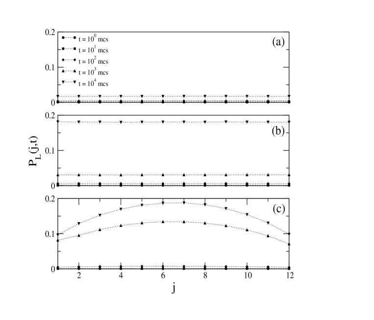
It is found [55] that for zero fields and assuming both PBC and OBC (Figure 8 (a)-(b), respectively), the damage profiles are essentially flat. This can be explained in terms of the interfaces between different magnetic domains which are essentially perpendicular to the film and the overall effect on the profiles is homogeneous. On the other hand, in presence of surface fields the situation is qualitatively different (see Figure 8(c)). The damage profiles show an important curvature related to the existence of an interface in the -direction, as shown in Figure 2(c). The effect of the walls is to slow down the propagation of the damage, while the interface between magnetic domains running along the film enhance the spreading of the damage.
5.2.2 Corner Geometry.
DS in the corner geometry, with competing (short-range) magnetic fields acting on the surfaces, shows [59] a behavior qualitatively similar to that the observed in the case of the strip geometry (see Figure 9). However, in contrast to the previous case, three different regimes for DS were found, as is shown in Figure 10. For short times, one observes the healing of the damage created in the bulk of the domains. However, at the critical DS point, a small cluster of damaged sites survives close to the interface. During the second time regime, the damage propagates along the interface according to a power-law behavior of the form , with . Finally, due to the constraint imposed by the corners where magnetic fields of opposite direction meet, the damage no longer propagates along the surface but starts to spread slowly into the bulk of the domains. Within this late regime one has , where is the exponent describing the spreading of the damage in the bulk [59].
As in the case of strip geometry, it is useful to gain further insight into the spatiotemporal propagation of the damage. For this purpose, the probability distribution of the distance from the damage zone to the corner () can be measured. The distribution was evaluated along the diagonal of the sample (-direction in Figure 4) at . Figure 11 shows a summary of the results [59].
In these cases, for (e.g. ) the distribution is almost flat with two small peaks close to the corners. Approaching the transition by increasing the field these peaks develop and become slightly shifted toward the center of the sample (e.g. and in Figure 11). This double-peaked structure indicates that the damage remains bound to each corner with the same probability as expected for the case of the non-wet phase. On the other hand, for (e.g. in Figure 11) the distribution becomes a Gaussian centered along the middle of the sample. The Gaussian structure of remains even for (e.g. in Figure 11). This results are in qualitative agreement with the corresponding to the damage profile showed in Figure 8 for the strip geometry; and it shows that the damage is located in the neighborhood of the interface between magnetic domains.
5.2.3 Overview of the Behaviour of DS in Different Confinement Geometries.
Table I summarizes the exponents obtained for different confinement geometries and boundary conditions. In view of the exponents obtained, one concludes that the presence of interfaces between magnetic domains of different orientation causes the enhancement of the propagation as compared with samples where such interfaces are not well defined. Furthermore, these results clearly show that the propagation of the damage is anisotropic: it propagates better along an interface than across it. Moreover, the obtained results suggest that the damage propagates along the magnetic interfaces with a critical exponent and it spreads into the magnetic domains with an exponent .
Taking into account this point of view, the value of the exponent can be explained in terms of the equilibrium configurations of the system. In fact, the sequence of domains with spins of opposite sign implies the inhomogeneity in the propagation of damage. When the perturbation arrives at an interface, it will propagate faster than in the bulk. For this reason, the exponent can be thought as a result of the interplay between the propagation along the interfaces and the propagation inside the magnetic domains. Regrettably, for this example it seems to be impossible to separate both effects in order to write the exponent in terms of and .
Figure 12 shows the behavior of for the different confinement geometries studied: the strip geometry with PBC’s and OBC’s at criticality and without applied magnetic fields [54, 55], the Abraham’s Model [56] and the corner geometry [59]. In all these cases and because of the dependence on the initial conditions, the first mcs were disregarded in order to evaluate the exponents.
| Model | Critical Exponent |
|---|---|
| Ising strip geometry with PBC [54] | |
| Ising strip geometry with OBC [54] | |
| Abraham’s Model [56] | |
| Corner Geometry (Second Regime) [59] | |
| Corner Geometry (Third Regime) [59] |
Table I. List of the critical exponent of Damage Spreading () obtained for the different models, as indicated in the first column.
6 Conclusions.
A brief overview of the Damage Spreading method applied to different models is presented and the critical non-equilibrium DS transition is analyzed. Within this context, DS in confined geometries is discussed in detail. A power-law behavior is found for DS as a function of time. The dynamic critical exponent depends on the presence of interfaces between magnetic domains generated by the existence of surface magnetic fields applied to the walls of the lattice. The results reported suggest that the damage propagates along the interfaces between domains with opposite orientations of the magnetization with an exponent and it spreads into the magnetic domain with an exponent . In view of these results, we conclude that the presence of interfaces enhances the propagation of a perturbation.
The critical propagation-nonpropagation transition of the damage was studied too. The results discussed indicate that, in some cases as in the Abraham’s model and a pure Ising system in the absence of magnetic fields, there is clear evidence indicating that the DS transition and the critical transition of the corresponding system occur at different critical points. These cases correspond to the wetting and the ferromagnet-paramagnet transitions, respectively. In the case of the corner geometry, both transitions damage spreading and corner-filling coincide within error bars.
In the cases of confined geometries, the critical exponents found suggest that the DS transition does not belong to the DP universality class. This finding seems to be related to the enhancement of the propagation of the damage caused by the magnetic interfaces appearing in confined samples.
The DS method is a suitable tool for the study and understanding of the propagation of perturbations in physical systems. Due to the concept of universality that allows one to describe second-order phase transitions and classify them into universality classes, characterized by the same set of critical exponents, it is possible to investigate simple models representing more complex physical situations, as e.g. the Ising model as archetype of various systems such as ferromagnets, fluids, lattice gases, binary alloys, etc. Therefore, the discussed role of the interfaces in the propagation of perturbations may be a quite general phenomenon of relevance in material science in general, and particularly, due to the additional influence of confinement, in the field of micro- and nanotechnology.
Acknowledgments. This work was supported financially by CONICET, UNLP, and ANPCyT (Argentina). MLRP acknowledges CONICET for the grant of a fellowship.
References
- [1] H. Hinrichsen, “Critical Phenomena in Nonequilibrium Systems”, Adv. Phys. 49, 815 (2000); arXiv: cond-mat/0001070 (2000).
- [2] S. A. Kauffman, J. Theor. Biol. 22, 437 (1969); Physica D 10, 145 (1984).
- [3] H. J. Herrmann, Physica A 168, 516 (1990).
- [4] K. Binder, “Introduction to Monte Carlo Methods I”, in “Monte Carlo and Molecular Dynamics of Condensed Matter Systems”, Vol 49, Chap. 5, pp 125, Eds. K. Binder and C. Cicotti, SIF, Bologna (1996).
- [5] K. Binder and D. Stauffer, in “Applications of the Monte Carlo method in Statistical Physics”, Chap. 1, Ed. K. Binder, 2nd Edn, Springer-Verlag, Germany (1987).
- [6] H. J. Herrmann, in “Computer Simulation Studies in Condensed Matter Physics II”, Eds. D. P. Landau, K. K. Mon, H. -B. Sch ttler, pp 56, Springer-Verlag, Berlin (1990).
- [7] S. R. Broadbent, J. M. Hammersley, Proc. Camb. Phil. Soc. 53, 629 (1957).
- [8] O. Martin, J. Stat. Phys. 41, 249 (1985).
- [9] B. Derrida, D. Stauffer, Europhys. Lett. 2, 739 (1986).
- [10] H. E. Stanley, D. Stauffer, J. Kertész, H. J. Herrmann, Phys. Rev. Lett. 59, 2326 (1987).
- [11] B. Derrida, G. Weisbuch, Europhys. Lett. 4, 657 (1987).
- [12] A. Coniglio, L. de Arcangelis, H. J. Herrmann, N. Jan, Europhys. Lett. 8 (4), 315 (1989).
- [13] U. M. S. Costa, J. Phys. A 20, L583 (1987).
- [14] G. Le Caër, J. Phys. A 22, L647 (1989); Physica A 159, 329 (1989).
- [15] A. M. Mariz, H. J. Herrmann, J. Phys. A 22, L1081 (1989),
- [16] S. C. Glotzer. D. Stauffer, S. Sastry, Physica A 164, 1 (1990).
- [17] A. M. Mariz, H. J. Herrmann, L. de Arcangelis, J. Stat. Phys. 59, 1043 (1990).
- [18] P. H. Poole, N. Jan, J. Phys. A 23, L453 (1990).
- [19] S. C. Glotzer. N. Jan, Physica A 173, 325 (1991).
- [20] F. D. Nobre, A. M. Mariz, E. S. Souza, Phys. Rev. Lett 69, 13 (1992).
- [21] S. C. Glotzer, P. H. Poole, N. Jan, J. Stat. Phys. 68, 895 (1992).
- [22] G. G. Batrouni, A. Hansen, J. Phys. A 25, L1059 (1992).
- [23] G-M. Zhang, C-Z. Yang, Europhys. Lett. 22, 505 (1993).
- [24] S. C. Glotzer, P. H. Poole, N. Jan, Phys. Rev. Lett. 70, 2046 (1993).
- [25] D. L. Hunter, L. de Arcangelis, R. Matz, P. H. Poole, N. Jan, Physica A 196, 188 (1993).
- [26] D. Stauffer, J. Phys. A 26, L599 (1993).
- [27] R. Matz, D. L. Hunter, N. Jan, J. Stat. Phys. 74, 903 (1994).
- [28] I. Graham, E. Hernández-García, M. Grant, Phys. Rev. E 49, R4763 (1994).
- [29] F. Tamarit, L. Da Silva, J. Phys. A 27, L809 (1994).
- [30] U. Gropengiesser, Physica A 207, 492 (1994).
- [31] P. Grassberger, Physica A 214, 547 (1995).
- [32] I. V. Rojdestvenski, U. M. S. Costa, Physica A 214, 485 (1995).
- [33] P. Grassberger, J. Phys. A 28, L67 (1995).
- [34] P. Grassberger, J. Stat. Phys. 79, 13 (1995).
- [35] U. Gropengiesser, Physica A 215, 308 (1995).
- [36] F. Montani, E. V. Albano, Phys. Lett. A 202, 253, (1995).
- [37] F. Wang, N. Hatano, M. Suzuki, J. Phys. A 28, 4543 (1995).
- [38] F. G. B. Moreira, A. J. F. Souza, A. M. Mariz, Phys. Rev. E 53, 332 (1996).
- [39] A. V. Lima, M. L. Lyra, U. M. S. Costa, J. Appl. Phys. 81 (8), 3983 (1997); J. Mag. Magn. Mat. 171, 329 (1997).
- [40] H. Hinrichsen, E. Domany, Phys. Rev. E 56, 94 (1997).
- [41] T. Vojta, J. Phys. A 30, L7 (1997).
- [42] T. Vojta, J. Phys. A 30, L643 (1997).
- [43] T. Vojta, Phys. Rev. E 55, 5157 (1997).
- [44] A. A. Júnior, F. D. Nobre, Physica A 243, 58 (1997).
- [45] T. Vojta, J. Phys. A 31, 6595 (1998).
- [46] T. Vojta, M. Schreiber, Phys. Rev. E 58, 7998 (1998).
- [47] Ubiraci P. C. Neves, J. R. Drugowich de Felício, Physica A 258, 211 (1998).
- [48] H. Hinrichsen, E. Domany, D. Stauffer, J. Stat. Phys. 91, 807 (1998).
- [49] C. Argolo, A. M. Mariz, S. M. Miyazima, Physica A 264, 142 (1999).
- [50] P. Gleiser, F. A. Tamarit, J. Phys. A 33, 6073 (2000).
- [51] C. Argolo, A. Mariz, M. Lyra, S. Miyazima, Phys. Rev. E 61, 1227 (2000).
- [52] C.-J. Liu, H.-B. Schüttler, J.-Z. Hu, Phys. Rev. E 65, 016114 (2001).
- [53] F. D. Nobre, A. A. Júnior, Phys. Lett. A 288, 271 (2001).
- [54] M. L. Rubio Puzzo, E. V. Albano, Physica A 293, 517 (2001).
- [55] M. L. Rubio Puzzo, E. V. Albano, J. Magn. Magn. Mat. 241, 110 (2002).
- [56] M. L. Rubio Puzzo, E. V. Albano, Phys. Rev. B 66, 104409 (2002).
- [57] T. Tomé, E. Arashiro, J. R. Drugowich de Felício, M. J. de Oliveira, Braz. Jour. of Phys. 33, 458 (2003); arXiv: cond-mat/0306410.
- [58] M. L. Rubio Puzzo, E. V. Albano, Physica A 349, 172 (2005).
- [59] M. L. Rubio Puzzo, E. V. Albano, J. Phys.: Cond. Matt. 19, 026201 (2007).
- [60] L. de Arcangelis, A. Coniglio, H. J. Herrmann, Europhys. Lett. 9, 749 (1989).
- [61] L. de Arcangelis, H. J. Herrmann, A. Coniglio, J. Phys. A 22, 4971 (1989).
- [62] H. R. da Cruz, U. M. S. Costa, E. M. F. Curado, J. Phys. A 22, L651 (1989).
- [63] N. Boissin, H. J. Herrmann, J. Phys. A 24, L43 (1991).
- [64] I. A. Campbell, L. de Arcangelis, Physica A 178, 29 (1991).
- [65] I. A. Campbell, Europhys. Lett. 21, 959 (1993).
- [66] I. A. Campbell, L. Bernardi, Phys. Rev. B 50, 12643 (1994).
- [67] R. M. C. de Almeida, L. Bernardi, I. A. Campbell, Journal de Physique 5, 355 (1995).
- [68] F. Wang, N. Kawashima, M. Suzuki, Europhys. Lett 33, 165 (1996).
- [69] T. Wappler, T. Vojta, M. Schreiber, Phys. Rev. B 55, 6272 (1997).
- [70] M. Heerema, F. Ritort, J. Phys. A 31, 8423 (1998); Phys. Rev. E 60, 3646 (1999).
- [71] A. Mariz, J. Phys. A. 23, 979 (1990).
- [72] M. F. A. Bibiano, F. G. B. Moreira, A. M. Mariz, Phys. Rev. E 55, 1448 (1997).
- [73] L. R. da Silva, F. A. Tamarit, A. C. N. de Magalhaes, J. Phys. A 30, 2329 (1997).
- [74] J. A. Redinz, F. A. Tamarit, A. C. N. de Magalhaes, Physica A 255, 439 (1998).
- [75] E. M. de Souza Luz, M. P. Almeida, U. M. S. Costa, M. L. Lyra, Physica A 282, 176 (2000).
- [76] J. A. Redinz, F. A. Tamarit, A. C. N. Magalhaes, Physica A 293, 508 (2001).
- [77] A. S. Anjos, D. A. Moreira, A. M. Mariz, F. D. Nobre, Phys. Rev. E 74, 016703 (2006).
- [78] E. N. Miranda, N. Parga, J. Phys. A 24, 1059 (1991).
- [79] U. M. S. Costa, A. F. de Souza, M. L. Lyra, Physica A 283, 42 (2000).
- [80] O. Golinelli, B. Derrida, J. Phys. A 22, L939 (1989).
- [81] J. Chiu, S. Teitel, J. Phys. A 23, L891 (1990).
- [82] A. M. Mariz, A. M. C. Souza, C. Tsallis, J. Phys. A 26, L1007 (1993).
- [83] Z. Z. Guo, K. Y. Szeto, X. Fu, Phys. Rev. E 70 , 016105 (2004).
- [84] Z. Z. Guo, K. Y. Szeto, Phys. Rev. E 71, 066115 (2005).
- [85] D. Stauffer, J. Stat. Phys. 74, 1293 (1994).
- [86] A. Valeriani, J. L. Vega, J. Phys. A 32, 105 (1999).
- [87] F. Bagnoli, R. Rechtman, S. Ruffo, Phys. Lett. A 172, 34 (1992).
- [88] C. Tsallis, F. A. Tamarit, A. M. C. de Souza, Phys. Rev. E 48, 1554 (1993).
- [89] C. Tsallis, M. L. Martins, EuroPhys. Lett. 27, 415 (1994).
- [90] T. Tomé, Physica A 212, 99 (1994).
- [91] H. Hinrichsen, J. S. Weitz, E. Domany, J. Stat. Phys. 88, 617 (1997).
- [92] R. A. Monetti, E. V. Albano, Phys. Rev. E 52, 5825 (1995); J. Theor. Biol. 187, 183 (1997).
- [93] F. Bagnoli, J. Stat. Phys. 85, 151 (1996).
- [94] E. N. Miranda, N. Parga, J. Phys. A 22, L907 (1989).
- [95] E. V. Albano, Phys. Rev. E 50, 1129 (1994).
- [96] E. V. Albano, Phys. Rev. Lett. 72, 108 (1994); J. Stat. Phys. 78, 1147 (1995); Physica A 215, 451 (1995).
- [97] A. Bhowal, Physica A 247, 327 (1997).
- [98] G. Ódor, N. Menyhárd, Phys. Rev. E 57, 5168 (1998).
- [99] P. Gleiser, Physica A 295, 311 (2001).
- [100] J. M. Kim, Y. Lee, I. Kim, Phys. Rev. E 54, 4603 (1996).
- [101] Y. Kim, C. K. Lee, Phys. Rev. E 62, 3376 (2000).
- [102] Y. Kim, Phys. Rev. E 64, 027101 (2001).
- [103] S. Fortunato, Physica A 348, 683, (2005).
- [104] N. Klietsch, Int. J. Mod. Phys. C 16, 4 (2004).
- [105] P. Svenson, D. A. Johnston, Phys. Rev. E 65, 036105 (2002).
- [106] N. G. F. Medeiros, A. T. C. Silva, F. G. Brady Moreira, Physica A 348, 691 (2005).
- [107] E. Domany, W. Kinzel, Phys. Rev. Lett. 53, 311 (1984).
- [108] W. Kinzel, Z. Phys. B 58, 229 (1985).
- [109] E. Ising, Z. Phys. 31, 253 (1925).
- [110] M. L. Martins, H. F. V. de Resende, C. Tsallis, A. C. N. de Magalh es, Phys. Rev. Lett. 66, 2045 (1991).
- [111] G. F. Zebende, T. J. P. Penna, J. Stat. Phys. 74, 1273 (1994).
- [112] M. L. Martins, G. F. Zebende, T. J. P. Penna, C. Tsallis, J. Phys. A 27, 1 (1994).
- [113] A. S. H. Rieger, M. Schreckenberg, J. Phys. A 27, L423 (1994).
- [114] G. A. Kohring, M. Schreckenberg, Journal de Physique 2, 2033 (1992).
- [115] N. Jan, L. de Arcangelis, in “Annual Review of Computational Physics I”, chap. 1, Ed. D. Stauffer, World Scientific, Singapore, 1994.
- [116] S. R. Broadbent, J. M. Hammersley, Proc. Camb. Phil. Soc. 53, 629 (1957).
- [117] I. Jensen, J. Phys. A 32, 5233 (1999).
- [118] C. A. Voigt, R. M. Ziff, Phys. Rev. E 56, R6241 (1997).
- [119] E. Domany, W. Kinzel, Phys. Rev. Lett. 53, 447 (1984).
- [120] R. Ziff, E. Gulari, Y. Barshad, Phys. Rev. Lett. 56, 2553 (1986).
- [121] E. S. Loscar, E. V. Albano, Rep. Prog. Phys. 66, 1343 (2003).
- [122] D. Abraham, Phys. Rev. Lett. 44, 1165 (1980).
- [123] H. Nakanishi, M. Fisher, Phys. Rev. Lett. 49, 1565 (1982).
- [124] K. Binder, D. P. Landau, J. Appl. Phys. 57, 3306 (1985).
- [125] K. Binder, D. P. Landau, D. M. Kroll, J. Magn. Magn. Matter. 54, 669 (1986); Phys. Rev. Lett. 56, 2272 (1986).
- [126] D. B. Abraham, in “Phase Transitions and Critical Phenomena”, Eds. C. Domb and J. L. Lebowitz, Vol 10 pp. 1, Academic New York (1987).
- [127] V. Privman, N. M. Svrakić, Phys. Rev. B 37, 3713 (1988).
- [128] E. V. Albano, K. Binder, D. W. Heermann, W. Paul, Surf. Sci. 223, 151 (1989); J. Chem. Phys 91, 3700 (1989); Z. Phys B 77, 445 (1989); J. Stat. Phys. 61, 161 (1990).
- [129] A. O. Parry, R. Evans, Phys. Rev. Lett. 64, 439 (1990).
- [130] A. O. Parry, R. Evans, Physica A 181, 250 (1992).
- [131] K. Binder, D. P. Landau, A. M. Ferrenberg, Phys. Rev. Lett. 74, 298 (1995); Phys. Rev. E 51, 2823 (1995).
- [132] A. Maciolek, J. Stecki, Phys. Rev. B 54, 1128 (1996).
- [133] A. Maciolek, J. Phys. A: Math. Gen. 29, 3837 (1996).
- [134] E. Carlon, A. Drzewinski, Phys. Rev. E 57, 2626 (1998).
- [135] A. M. Ferrenberg, D. P. Landau, K. Binder, Phys. Rev. E 58, 3353 (1998).
- [136] E. V. Albano, K. Binder, W. Paul, J. Phys. C 12, 2701 (2000).
- [137] K. Binder, D. Landau, M. Miller, J. Stat. Phys. 110, 1411 (2003).
- [138] P. M. Duxbury, A. C. Orrick, Phys. Rev. B 39, 2944 (1989).
- [139] E. Cheng, M. W. Cole, Phys. Rev. B 41, 9650 (1990).
- [140] M. Napiórkowsi, W. Koch, S. Dietrich, Phys. Rev. A 45, 5760 (1992).
- [141] E. H. Hauge, Phys. Rev. A 46, 4994 (1992).
- [142] A. Lipowski, Phys. Rev. E 58, R1 (1998).
- [143] K. Rejmer, S. Dietrich, M. Napiorkowski, Phys. Rev. E 60, 4027 (1999).
- [144] A. O. Parry, C. Rascón, A. J. Wood, Phys. Rev. Lett. 83, 5535 (1999).
- [145] A. O. Parry, A. J. Wood, C. Rascón, J. Phys. C 12, 7671 (2000).
- [146] M. Gleiche, L. F. Chui, H. Fuchs, Nature 403, 173 (2000).
- [147] C. Rascón, A. O. Parry, Nature 407, 986 (2000).
- [148] A. O. Parry, C. Rascón, A. J. Wood, Phys. Rev. Lett. 85, 345 (2000).
- [149] A. Bednorz, M. Napiórkowsi, Phys. Rev. E 63, 031602 (2001); J. Phys. A 33, L353 (2001).
- [150] A. O. Parry, A. J. Wood, E. Carlon, A. Drzewiński, Phys. Rev. Lett. 87, 196103 (2001).
- [151] A. O. Parry, A. J. Wood, C. Rascón, J. Phys. C 13, 4591 (2001).
- [152] D. B. Abraham, A. O. Parry, A. J. Wood, Europhys. Lett. 60, 106 (2002).
- [153] D. B. Abraham, A. Maciolek, Phys. Rev. Lett. 89, 286101 (2002).
- [154] A. O. Parry, M. J. Greenall, A. J. Wood, J. Phys. C 14, 1169 (2002).
- [155] A. Sartori, A. O. Parry, J. Phys. C 14, L679 (2002).
- [156] D. B. Abraham, V. Mustonen, A. J. Wood, Europhys. Lett. 63, 408 (2003).
- [157] E. V. Albano, A. de Virgiliis, M. Müller, K. Binder, J. Phys. C 15, 333 (2003).
- [158] A. Milchev, M. Müller, K. Binder, D. P. Landau, Phys. Rev. Lett. 90, 136101 (2003); Phys. Rev. E 68, 031601 (2003).
- [159] A. O. Parry, J. M. Romero-Enrique, A. Lazarides, Phys. Rev. Lett. 93, 086104 (2004).
- [160] J. M. Romero-Enrique, A. O. Parry, M. J. Greenall, Phys. Rev. E 69, 061604 (2004).
- [161] J. M. Romero-Enrique, A. O. Parry, J. Phys. C 17, S3487 (2005).
- [162] J. M. Romero-Enrique, A. O. Parry, Europhys. Lett. 72, 1004 (2005).
- [163] D. B. Abraham and A. Maciolek, Phys. Rev. E 72, 031601 (2005).
- [164] K. Rejmer, Phys. Rev. E 71, 011605 (2005).
- [165] C. Rascón, A. O. Parry, Phys. Rev. Lett. 94, 096103 (2005).
- [166] G. Giugliarelli, Phys. Rev. E 71, 021603 (2005).
- [167] M. Müller, K. Binder, J. Phys. C 17, S333 (2005).
- [168] V. Manias, J. Candia, E. V. Albano, Eur. Phys. J. B. 47, 563 (2005).