Decoy states for quantum key distribution based on decoherence-free subspaces

Abstract

Quantum key distribution with decoherence-free subspaces has been proposed to overcome the collective noise to the polarization modes of photons flying in quantum channel. Prototype of this scheme have also been achieved with parametric-down conversion source. However, a novel type of photon-number-splitting attack we proposed in this paper will make the practical implementations of this scheme insecure since the parametric-down conversion source may emit multi-photon pairs occasionally. We propose decoy states method to make these implementations immune to this attack. And with this decoy states method, both the security distance and key bit rate will be increased.

I introduction

As a combination of quantum mechanics and conventional cryptography, Quantum Key Distribution (QKD) BB84 ; ekert1991 ; Gisin , can help two distant peers (Alice and Bob) share secret string of bits, called key. Unlike conventional cryptography whose security is based on computation complexity, the security of QKD relies on the fundamental laws of quantum mechanics. Any eavesdropping attempt to an ideal QKD process will introduce an abnormal high bit error rate of the key. By comparing subset of the key, Alice and Bob can catch any eavesdropping attempt. Polarization and phase time of photons are the most common coding method to implement QKD. But, birefringence in optical fiber may depolarize the photons, which makes the polarization coding unsuitable for QKD based on fiber. Phase time coding is commonly used for fiber QKD. Using ”Plug&Play” Gisin or Faraday-Michelson interferometersF-M , phase time coding can be free from polarization fluctuations due to birefringence of optical fiber. However, ”Plug&Play” may be vulnerable for Trojan attack. And for Faraday-Michelson interferometers F-M , it’s very sensitive to phase fluctuations from arms between Alice’s and Bob’s interferometers. To overcome this problem, active compensation which makes the system more complicated and unefficient is used.

Alternatively, Walton $et$ $al.$ Walton proposed a novel QKD protocol based on decoherence-free space (DFS) and Boileau $et$ $al.$ Boileau developed this scheme to use time-bin and polarization for encoding. In Boileau’s scheme, Alice can encode her qubit in the two-photon states as follows: $|H\rangle|V\rangle$, $|V\rangle|H\rangle$, $(|H\rangle|V\rangle+|V\rangle|H\rangle)/\sqrt{2}$, and $(|H\rangle|V\rangle-|V\rangle|H\rangle/\sqrt{2}$, (in experiment by J.-W. Pan DFS experiment , the four states are: $(|H\rangle|V\rangle+|V\rangle|H\rangle)/\sqrt{2}$, $(|H\rangle|V\rangle-|V\rangle|H\rangle)/\sqrt{2}$, $(|H\rangle|V\rangle+i|V\rangle|H\rangle)/\sqrt{2}$ and $(|H\rangle|V\rangle-i|V\rangle|H\rangle/\sqrt{2}$), where $H(V)$ means the horizontal (vertical) polarization mode of photons. The two photons are distinguishable by a fixed time delay $\Delta t_{p}$, which is known to Alice and Bob. Then Alice applies a time delay operation to the $V$ photons and before Bob detects the two photons, he applies a same time delay operation to the $H$ photons. Finally, Bob detects the two photons in the $|H\rangle|V\rangle$, $|V\rangle|H\rangle$ basis or $\frac{1}{\sqrt{2}}(|H\rangle|V\rangle+|V\rangle|H\rangle)$, $\frac{1}{\sqrt{2}}(|H\rangle|V\rangle-|V\rangle|H\rangle$ basis. Due to the fact that $|\psi^{-}\rangle=\frac{1}{\sqrt{2}}(|H\rangle|V\rangle-|V\rangle|H\rangle)$ is invariant under collective unitary transformation, this scheme is insensitive to phase fluctuations from Alice’s and Bob’s interferometers. If the interval of the time between the two photons is just $\Delta t_{p}$, Bob will successfully get Alice’s qubit and this probability will be $2/3$ assuming the collective noise is totally random. Besides this, photons from the same pair can provide precise time references for each other. So in this scheme, accurate synchronization clock is unnecessary.

BB84-type QKD protocols which are the most-widely used QKD protocol, needs single photon source which is not practical for present technology. Usually, real-file QKD set-ups qkd1 ; qkd2 ; qkd3 ; qkd4 ; F-M use attenuated laser pulses (weak coherent states) instead. It means the laser source is equivalent to a one that emits n-photon state $|n\rangle$ with probability $P_{n}=\frac{\mu^{n}}{n!}e^{-\mu}$, where $\mu$ is average photon number of the attenuated lased pulses. This photon number Poisson distribution stems from the coherent state $|\sqrt{\mu}e^{i\theta}\rangle$ of laser pulse. Therefore, a few multi-photon events in the laser pulses emitted from Alice open the door of Photon-Number-Splitting attack (PNS attack) PNS1 ; PNS2 ; PNS3 which makes the whole QKD process insecure. Fortunately, decoy states QKD theory decoy theory1 ; decoy theory2 ; decoy theory3 ; decoy theory4 ; decoy theory5 , as a good solution to beat PNS attack, has been proposed. And some prototypes of decoy state QKD have been implemented decoy experiment1 ; decoy experiment2 ; decoy experiment3 ; decoy experiment4 ; decoy experiment5 ; decoy experiment6 ; decoy experiment7 . The key point of decoy states QKD is to calculate the lower bound of counting rate of single-photon pulses ($S_{1}^{L}$) and upper bound of quantum bit error rate (QBER) of bits generated by single-photon pulses ($e_{1}^{U}$). Many methods to improve performance of decoy states QKD have been presented, including more decoy states decoy theory5 , nonorthogonal decoy-state method nonorthogonal state protocol , photon-number-resolving method photon-number-resolving method , herald single photon source method herald1 ; herald2 , modified coherent state source method MCS . And for the intensity fluctuations of the laser pulses, Ref. intensity error1 and intensity error2 give good solutions.

As a BB84-type protocol, Boileau’s scheme is still vulnerable to PNS attack. This problem will be discussed in details in the section II, in which we propose a novel type of PNS attack. In the Section III, we propose a decoy states method to overcome this problem. In Section IV, a numerical simulation will be given. Finally, we will give a summary to end this paper.

II PNS attack in Boileau’s scheme

To implement Boileau’s scheme, an ideal two-photon states source which is far from present technology, is needed. In practice, two-photon states are generated by parametric down-conversion source(PDCS), which will emit n-photon ($n>1$) pairs with certain probability. However, the state from a type-II PDCS can be written like PDCS :

$$|\psiup\rangle=(\cosh\chi)^{-2}\sum_{n=0}^{\infty}\sqrt{n+1}e^{in\theta}\tanh^{n}\chi|\Phi_{n}\rangle,$$ (1)

in which, $|\Phi_{n}\rangle$ is the state of n-photon pair, given by:

$$|\Phi_{n}\rangle=\frac{1}{\sqrt{n+1}}\sum_{m=0}^{n}(-1)^{m}|n-m,m\rangle_{a}|m,n-m\rangle_{b}$$ (2)

Here, $|n,m\rangle_{a(b)}=|H\rangle^{\otimes n}_{a(b)}|V\rangle^{\otimes m}_{a(b)}$, a, b means the two spatial output modes of PDCS respectively. By randomizing the phase $\theta$ decoy theory1 , we can write the density matrix of the PDCS as $\rho_{\lambda}=\int(d\theta/(2\pi))|\psiup\rangle\langle\psiup|=P_{n}(\lambda)|\Phi_{n}\rangle\langle\Phi_{n}|$, where, $P_{n}(\lambda)=(n+1)\lambda^{n}/(1+\lambda)^{n+2}$, $\lambda=\sinh^{2}\chi$, which is half of the average number of photon pairs generated by one pumping pulse and could be adjusted by the intensity of the pumping pulsed. Therefore, PDCS is really just a photon-number states source emitting n-photon pairs $|\Phi_{n}\rangle$ with probability $P_{n}(\lambda)$. For implementations that do not apply phase randomization, Eve may attack this QKD system more powerfully phase randomization , Therefore, for simplicity we assume that Alice have applied phase randomization to her photon pairs.

Here we focus on the attack to 2-photon pairs, because the 2-photon pairs are dominant among the multi-photon pairs. For the practical implementation DFS experiment by Pan, Alice delays b mode of the two spatial outputs of PDCS with $\Delta t_{p}$. Then through phase-modulation by Pockel cells DFS experiment 2-photon pairs states could be described in creation operators form like this:

$$|-\rangle=\frac{1}{2\sqrt{3}}({H_{a}^{+}}^{2}{V_{b}^{+}}^{2}-2H_{a}^{+}V_{a}^{+}H_{b}^{+}V_{b}^{+}+{V_{a}^{+}}^{2}{H_{b}^{+}}^{2})|vacuum\rangle$$ (3)

$$|+\rangle=\frac{1}{2\sqrt{3}}({H_{a}^{+}}^{2}{V_{b}^{+}}^{2}+2H_{a}^{+}V_{a}^{+}H_{b}^{+}V_{b}^{+}+{V_{a}^{+}}^{2}{H_{b}^{+}}^{2})|vacuum\rangle$$

$$|0\rangle=\frac{1}{2\sqrt{3}}({H_{a}^{+}}^{2}{V_{b}^{+}}^{2}+2iH_{a}^{+}V_{a}^{+}H_{b}^{+}V_{b}^{+}-{V_{a}^{+}}^{2}{H_{b}^{+}}^{2})|vacuum\rangle$$

$$|1\rangle=\frac{1}{2\sqrt{3}}({H_{a}^{+}}^{2}{V_{b}^{+}}^{2}-2iH_{a}^{+}V_{a}^{+}H_{b}^{+}V_{b}^{+}-{V_{a}^{+}}^{2}{H_{b}^{+}}^{2})|vacuum\rangle$$

where, $H_{a}^{+}$, $H_{b}^{+}$, $V_{a}^{+}$, and $V_{b}^{+}$ represent the creation operators for horizontal polarized photons in $a$ mode, horizontal polarized photons in $b$ mode, vertical polarized photons in $a$ mode and vertical polarized photons in $b$ mode. For simplicity, we assume Eve add a beam splitter (BS) to the both modes $a$ and $b$ and we name the two spatial mode of the output of the BS is $1$ and $2$. Now Eve has 4 spatial-temporal modes $a1$, $a2$, $b1$ and $b2$, and creator operators for horizontal-polarized and vertical-polarized photons in these new modes are correlated to modes $a$ and $b$ by $H_{a}^{+}=(1/\sqrt{2})(H_{a1}^{+}-H_{a2}^{+})$, $V_{a}^{+}=(1/\sqrt{2})(V_{a1}^{+}-V_{a2}^{+})$, $H_{b}^{+}=(1/\sqrt{2})(H_{b1}^{+}-H_{b2}^{+})$, and $V_{a}^{+}=(1/\sqrt{2})(V_{b1}^{+}-V_{b2}^{+})$. Then Eve can post-select the states that each of modes $a1$, $b1$ $a2$ and $b2$ has one and only one photon respectively. We should notice that: although through just one BS the probability of success of this post-selection is just 1/4, Eve may use many BSs to make sure that this probability will be close to 1. And states $|-\rangle$, $|+\rangle$, $|0\rangle$ and $|1\rangle$ will be transformed to:

$$|-\rangle^{\prime}=\frac{1}{2\sqrt{2}}((H_{a1}V_{b1}-V_{a1}H_{b1})(H_{a2}V_{b2}-V_{a2}H_{b2})$$ (4)

$$+(H_{a1}V_{b2}-V_{a1}H_{b2})(H_{a2}V_{b1}-V_{a2}H_{b1}))$$

$$|+\rangle^{\prime}=\frac{1}{2\sqrt{2}}((H_{a1}V_{b1}+V_{a1}H_{b1})(H_{a2}V_{b2}+V_{a2}H_{b2})$$

$$+(H_{a1}V_{b2}+V_{a1}H_{b2})(H_{a2}V_{b1}+V_{a2}H_{b1}))$$

$$|0\rangle^{\prime}=\frac{1}{2\sqrt{2}}((H_{a1}V_{b1}+iV_{a1}H_{b1})(H_{a2}V_{b2}+iV_{a2}H_{b2})$$

$$+(H_{a1}V_{b2}+iV_{a1}H_{b2})(H_{a2}V_{b1}+iV_{a2}H_{b1}))$$

$$|1\rangle^{\prime}=\frac{1}{2\sqrt{2}}((H_{a1}V_{b1}-iV_{a1}H_{b1})(H_{a2}V_{b2}-iV_{a2}H_{b2})$$

$$+(H_{a1}V_{b2}-iV_{a1}H_{b2})(H_{a2}V_{b1}-iV_{a2}H_{b1}))$$

where $H(V)_{X}$ represents state vector $|H(V)\rangle_{X}$ for abbreviation and the same below. Then Eve could use a unitary transformation $\mathscr{U}_{1}$ to the photons in modes $a1$ and $b2$. The definition of $\mathscr{U}_{1}$ is given by $\mathscr{U}_{1}HVE_{0}=HVE_{1}$, $\mathscr{U}_{1}VHE_{0}=VHE_{1}$, $\mathscr{U}_{1}HHE_{0}=HHE_{2}$ and $\mathscr{U}_{1}VVE_{0}=VVE_{2}$, in which $E_{x}$ is an assist state of Eve and satisfying $\langle E_{0}|E_{1}\rangle=\langle E_{0}|E_{2}\rangle=\langle E_{1}|E_{2}\rangle=0$. Eve post-select $E_{1}$ through projection $P_{1}=|E_{1}\rangle\langle E_{1}|$ and then the four states will be mapped into the below states with probability $75\%$.

$$|-\rangle^{\prime\prime}=\frac{1}{\sqrt{5}}(2|X\rangle-|Y\rangle)$$ (5)

$$|+\rangle^{\prime\prime}=\frac{1}{\sqrt{5}}(2|X\rangle+|Y\rangle)$$

$$|0\rangle^{\prime\prime}=\frac{1}{\sqrt{5}}(2|X^{\prime}\rangle+i|Y\rangle)$$

$$|1\rangle^{\prime\prime}=\frac{1}{\sqrt{5}}(2|X^{\prime}\rangle+i|Y\rangle)$$

where, $|X\rangle=(1/\sqrt{2})(H_{a1}V_{b1}H_{a2}V_{b2}+V_{a1}H_{b1}V_{a2}H_{b2})$, $|Y\rangle=(1/\sqrt{2})(H_{a1}H_{b1}V_{a2}V_{b2}+V_{a1}V_{b1}H_{a2}H_{b2})$ and $|X^{\prime}\rangle=(1/\sqrt{2})(H_{a1}V_{b1}H_{a2}V_{b2}-V_{a1}H_{b1}V_{a2}H_{b2})$. Now, Eve can construct another unitary transformation $\mathscr{U}_{2}$ defined by: $\mathscr{U}_{2}|X\rangle|E_{0}\rangle=(\sqrt{3}|Z\rangle|E_{1}\rangle+|X\rangle|E_{2}\rangle)/2$, $\mathscr{U}_{2}|X^{\prime}\rangle|E_{0}\rangle=(\sqrt{3}|Z\rangle|E_{3}\rangle+|X^{\prime}\rangle|E_{2}\rangle)/2$ and $\mathscr{U}_{2}|Y\rangle|E_{0}\rangle=|Y\rangle|E_{2}\rangle$. Here, $|E\rangle$ represents an assist states of Eve and $\langle E_{0}|E_{1}\rangle=\langle E_{0}|E_{2}\rangle=\langle E_{1}|E_{2}\rangle=0$. And $|Z\rangle$ is any states of photon in modes $a1$, $b1$, $a2$ and $b2$. With $\mathscr{U}_{2}$ and projection operation $P_{2}=|E_{2}\rangle\langle E_{2}|$, the four photon states will be mapped to the followed form with probability 40%.

$$|-\rangle^{\prime\prime\prime} =\frac{1}{\sqrt{2}}(|X\rangle-|Y\rangle)$$ (6)

$$=\frac{1}{\sqrt{2}}(H_{a1}V_{b2}-V_{a1}H_{b2})\frac{1}{\sqrt{2}}(H_{a2}V_{b1}-V_{a2}H_{b1})$$

$$|+\rangle^{\prime\prime\prime} =\frac{1}{\sqrt{2}}(|X\rangle+|Y\rangle)$$

$$=\frac{1}{\sqrt{2}}(H_{a1}V_{b2}+V_{a1}H_{b2})\frac{1}{\sqrt{2}}(H_{a2}V_{b1}+V_{a2}H_{b1})$$

$$|0\rangle^{\prime\prime\prime} =\frac{1}{\sqrt{2}}(|X\rangle+i|Y\rangle)$$

$$=\frac{1}{\sqrt{2}}(H_{a1}V_{b2}+iV_{a1}H_{b2})\frac{1}{\sqrt{2}}(H_{a2}V_{b1}+iV_{a2}H_{b1})$$

$$|1\rangle^{\prime\prime\prime} =\frac{1}{\sqrt{2}}(|X\rangle-i|Y\rangle)$$

$$=\frac{1}{\sqrt{2}}(H_{a1}V_{b2}-iV_{a1}H_{b2})\frac{1}{\sqrt{2}}(H_{a2}V_{b1}-iV_{a2}H_{b1})$$

Obviously, with the states $|-\rangle^{\prime\prime\prime}$, $|+\rangle^{\prime\prime\prime}$, $|0\rangle^{\prime\prime\prime}$ and $|1\rangle^{\prime\prime\prime}$, Eve can keep one pair and send the other pair to Bob through a special channel controlled by herself. When Alice and Bob do basis reconciliation, Eve will get all secret information. This is just the same as PNS attack PNS1 ; PNS2 ; PNS3 .

Let us review our attack strategy. First, Eve divides the two photons in modes $a$ and $b$ into modes $a1$, $a2$ and $b1$, $b2$ respectively. With many BSs, success probability of this step is close to 1. Second, Eve applys unitary transformation $\mathscr{U}_{1}$ and projection $P_{1}$, she gets an intermediate state with success probability $75\%$. Finally, She applys unitary transformation $\mathscr{U}_{2}$ and projection $P_{2}$, she gets the final state which she can launch PNS attack immediately and success probability of this step is $40\%$. Overall, for 2-photon pairs Eve will launch PNS attack with probability of $75\%\times 40\%=30\%$ or discard a failure case with probability $1-30\%=70\%$.

According to the above fact and the discussion of Ref. PNS1 ; PNS2 ; PNS3 , we know the security distance ($L$) of this scheme must obey $P_{1}(\lambda)(10^{-kL/10})^{2}\geq P_{2}(\lambda)\times 30\%$ in which $k$ is the transmission fiber loss constance. If we assume $k=0.2dB/km$ which is a typical value of this constance and $\lambda=0.1$, we obtain $L\leqq 37.4km$. This is a highly unsatisfactory situation. How to prolong the security distance is what we will discuss in the next section.

III Decoy states to Boileau’s scheme

The rate of secret key bits ($R$) for BB84 protocol with nonideal source can be determined by GLLP GLLP :

$$R\geqslant R^{L}=q[-Q_{\lambda}f(E_{\lambda})H_{2}(E_{\lambda})+P_{1}(\lambda)S_{1}^{L}(1-H_{2}(e_{1}^{U}))]$$ (7)

Here, $R^{L}$ represents the lower bound of $R$, q depends on protocol ($1/2$ for Boileau’s scheme), $Q_{\lambda}$ is the overall counting rate for the photon pairs, $\lambda$ is half of the average number of the photon pairs, $f(E_{\lambda})$ is error correction efficiency, $E_{\lambda}$ is the quantum bit error rate (QBER) of the key bit, $H_{2}$ is the binary Shannon information function, $S_{1}$ is the counting rate for the 1-photon pairs, and $e_{1}$ is the QBER of the key bits generated by the 1-photon pairs. Similar to BB84 based on weak coherent states, we need to modulate $\lambda$ to several values randomly. Through watching counting rates for different $\lambda$, we can obtain the lower bound of $S_{1}$ ($S_{1}^{L}$) and the upper bound of $e_{1}$ ($e_{1}^{U}$). Finally, $R^{L}$ can be obtained by equation (7).

Our 3-intensity protocol is: Alice randomly emits photon pairs of density matrix $\rho_{\lambda}$, $\rho_{\lambda^{\prime}}$, and $0$ ($\lambda$ for signal states , $\lambda^{\prime}$ ($\lambda>\lambda^{\prime}$) and $0$ for decoy states) , then Bob can get their counting rates $Q_{\lambda}$, $Q_{\lambda^{\prime}}$ and $S_{0}$. With formulas we derived later, $S_{1}^{L}$ and $e_{1}^{U}$ can be obtained. Finally, $R^{L}$ is given by equation (7). Now we drive these formulas.

The counting rates for the two intensity ($\lambda$ and $\lambda^{\prime}$) photon pairs is determined by:

$$Q_{\lambda}=\sum_{n=0}^{\infty}P_{n}(\lambda)S_{n}$$ (8)

$$Q_{\lambda^{\prime}}=\sum_{n=0}^{\infty}P_{n}(\lambda^{\prime})S_{n}$$ (9)

where, $S_{n}$ represents the counting rate for n-photon pair states $|\Phi_{n}\rangle$. Then QBER for the $\lambda$ ($E_{\lambda}$) is determined by:

$$E_{\lambda}Q_{\lambda}=\sum_{n=0}^{\infty}e_{n}P_{n}(\lambda)S_{n}$$ (10)

In which, $e_{n}$ is the QBER of the key bits generated by the n-photon pairs $|\Phi_{n}\rangle$. Before the derivation of the formula to calculate $S_{1}^{L}$ and $e_{1}^{U}$, we prove that $\frac{P_{2}(\lambda)}{P_{2}(\lambda^{\prime})}P_{n}(\lambda^{\prime})\leqslant P_{n}(\lambda)$ for all of $n\geqslant 2$.

$$\frac{P_{2}(\lambda)}{P_{n}{(\lambda)}}-\frac{P_{2}(\lambda^{\prime})}{P_{n}{(\lambda^{\prime}})}$$ (11)

$$=\frac{3}{n+1}((1+\frac{1}{\lambda})^{n-2}-(1+\frac{1}{\lambda^{\prime}})^{n-2}) \leqslant 0$$

With this result, we can deduce the formula for calculating $S_{1}^{L}$:

$$Q_{\lambda} =P_{0}(\lambda)S_{0}+P_{1}(\lambda)S_{1}+P_{2}(\lambda)S_{2}+P_{3}(\lambda)S_{3}+\cdots$$ (12)

$$\geqslant P_{0}(\lambda)S_{0}+P_{1}(\lambda)S_{1}+\frac{P_{2}(\lambda)}{P_{2}(\lambda^{\prime})}\sum_{n=2}^{\infty}P_{n}(\lambda^{\prime})S_{n}$$

With equation (9), we have:

$$S_{1}^{L}=\frac{(P_{2}(\lambda^{\prime})P_{0}(\lambda)-P_{2}(\lambda)P_{0}(\lambda^{\prime}))S_{0}+P_{2}(\lambda)Q_{\lambda^{\prime}}-P_{2}(\lambda^{\prime})Q_{\lambda}}{P_{2}(\lambda)P_{1}(\lambda^{\prime})-P_{2}(\lambda^{\prime})P_{1}(\lambda)}$$ (13)

According to equation (10) and decoy theory4 , $e_{1}^{U}$ can be given by:

$$e_{1}^{U}=\frac{(E_{\lambda}Q_{\lambda}-\frac{S_{0}P_{0}(\lambda)}{2})}{P_{1}(\lambda)S_{1}^{L}}$$ (14)

With equation (13) and (14), $S_{1}^{L}$ and $e_{1}^{U}$ can be obtained. Finally, $R^{L}$ is given by equation (7).

For experiment, 2-intensity decoy states protocol is quite convenient decoy experiment7 . In this case, Alice randomly emits photon pairs of density matrix $\rho_{\lambda}$ for signal states, $\rho_{\lambda^{\prime}}$ for decoy states, then Bob can get their counting rates $Q_{\lambda}$, $Q_{\lambda^{\prime}}$. We now deduce the formula to calculate $S_{1}^{L}$ and $e_{1}^{U}$ just from $Q_{\lambda}$, $Q_{\lambda^{\prime}}$.

According to equation (10), the upper bound of $S_{0}$ ($S_{0}^{U}$) can be given by:

$$S_{0}^{U}=\frac{2E_{\lambda}Q_{\lambda}}{P_{0}(\lambda)}$$ (15)

Then from equation (10), $S_{1}^{L}$ for two-intensity case can be given by:

$$S_{1}^{L}$$ (16)

$$=\frac{2(P_{2}(\lambda^{\prime})P_{0}(\lambda)-P_{2}(\lambda)P_{0}(\lambda^{\prime}))\frac{E_{\lambda}Q_{\lambda}}{P_{0}(\lambda)}+P_{2}(\lambda)Q_{\lambda^{\prime}}-P_{2}(\lambda^{\prime})Q_{\lambda}}{(P_{2}(\lambda)P_{1}(\lambda^{\prime})-P_{2}(\lambda^{\prime})P_{1}(\lambda))P_{0}(\lambda)}$$

To get $e_{1}^{U}$ for two intensity case, we just set lower bound of $S_{0}$ ($S_{0}^{L}$) to be $0$, then with equation (10) and (16), $e_{1}^{U}$ is given by:

$$e_{1}^{U}=\frac{E_{\lambda}Q_{\lambda}}{P_{1}(\lambda)S_{1}^{L}}$$ (17)

Equations (16) and (17) are for 2-intensity case. With these equations, we have established the basic methods to beat PNS attack in Boileau’s QKD scheme. Next, we will make sure that this decoy states method can improve the performance of Boileau’s QKD scheme impressively.

IV improvement by decoy states

Now, we will show the improvement for the performance by the introduction of decoy states through the numerical simulations. In the followed discussions and simulations, we neglect the error induced by channel and assume Bob’s measurements are perfect except a few dark counts for simplicity. According to Ref. DFS experiment , Bob’s measurement is equivalent to the projection to the polarization states $F$ and $S$ defined by $H=(F+S)/\sqrt{2}$ and $V=(F-S)/\sqrt{2}$ respectively. We rewrite the encoding states $|+\rangle$ and $|-\rangle$ in the form of $F$ and $S$: $|+\rangle=\frac{1}{\sqrt{n+1}}\sum_{m=0}^{n}(-1)^{m}F_{a}^{n-m}S_{a}^{m}F_{b}^{n-m}S_{a}^{m}$, $|-\rangle=\frac{1}{\sqrt{n+1}}\sum_{m=0}^{n}(-1)^{m}F_{a}^{n-m}S_{a}^{m}F_{b}^{m}S_{a}^{n-m}$. For Bob, if he observers the $F_{a}S_{b}$ or $S_{a}F_{b}$, it’s will be $|+\rangle$ while the $F_{a}F_{b}$ or $S_{a}S_{b}$ is for the result of $|+\rangle$. According to Ref.decoy theory4 , the transmission efficiency for the n-photon pulses $\eta_{n}$ can be written as $\eta_{n}=1-(1-\eta)^{n}$, in which $\eta$ is the transmission efficiency of the fiber channel and $\eta=10^{(-kL/10)}$, $K$ is the transmission fiber loss constance and L is the fiber length. Since our goal is to show the difference between the original Boileau’s scheme and this scheme with decoy states but not the exact $R^{L}$ verse fiber length, we take the efficiency of the detector and loss due to projection to the DFS space or other causes just as a part of fiber loss and don’t care these values. We assume the dark counting rates of the detectors is $D$. Since Bob must neglect all the three or four folds counts, $S_{n}$ can be written as:

$$S_{n} =\frac{(1-D)^{2}}{n+1}\sum_{m=0}^{n}((\eta_{n-m}(1-\eta)^{m}+\eta_{m}(1-\eta)^{n-m})^{2}$$ (18)

$$+4\eta_{n-m}(1-\eta)^{m}(1-\eta)^{n}D+4\eta_{m}(1-\eta)^{n-m}(1-\eta)^{n}D$$

$$+4(1-\eta)^{2n}D^{2})$$

Then with equation (8), we can get the formulas to estimate the $Q_{\lambda}$ and $Q_{\lambda^{\prime}}$.

$$Q_{\lambda} =\sum_{n=0}^{\infty}P_{n}(\lambda)S_{n}$$ (19)

$$=\frac{2(1-D)^{2}}{(1+\lambda\eta(3-\eta)+\lambda^{2}\eta^{2}(2-\eta))^{2}}\times$$

$$(4\lambda\eta D(1-\eta)(1+\lambda\eta)+2D^{2}(1+\lambda\eta)^{2}$$

$$+\lambda\eta^{2}(1+\lambda^{2}(2-\eta)\eta+\lambda(\eta^{2}-2\eta+3)))$$

For simplicity we neglect the probability that a survived photon hitting a wrong detector, then $e_{n}$ is written like:

$$e_{n}S_{n} =[\sum_{m=0}^{n}(2\eta_{n-m}(1-\eta)^{m}(1-\eta)^{n-m}\eta_{m}+2\eta_{m}(1-\eta)^{n-m}(1-\eta)^{n}D$$ (20)

$$+2\eta_{n-m}(1-\eta)^{m}(1-\eta)^{n}D+(1-\eta)^{2n}2D]\frac{(1-D)^{2}}{n+1}$$

in which, the first term of the summation corresponds to the case of the photons in modes $a$ and $b$ both hitting the detectors. Only when $n\geqslant 2$, this term does not equal to 0. The second and third terms in above summation represent to the case photons in only one mode ($a$ or $b$) hit the detector. The dark count of one detector may result in QBER in this situation. The last term of the summation is for the case of all the photons are absorded by fiber.

With this, we can estimate the QBER $E_{\lambda}$ as:

$$E_{\lambda} =\sum_{n=0}^{\infty}P_{n}(\lambda)e_{n}S_{n}/Q_{\lambda}$$ (21)

$$=(D+\lambda D\eta+\lambda\eta(1-\eta))^{2}\times$$

$$[4\lambda D\eta(1-\eta)(1+\lambda\eta)+2D^{2}(1+\lambda\eta)^{2}$$

$$+\lambda\eta^{2}(1+\lambda^{2}\eta(2-\eta)+\lambda(\eta^{2}-2\eta+3))]^{-1}$$

Now with equations (19) and (21) and setting $k=0.2dB/km$, $D=10^{-6}/pulse$, and $f(E_{\lambda})=1.2$, the $Q_{\lambda}$, $Q_{\lambda^{\prime}}$, $E_{\lambda}$ can be calculated by numerical simulations. Then with equations (13) and (14), the $S_{1}^{L}$ and $e_{1}^{U}$ can be obtained. Finally, the relation between $R^{L}$ and fiber length $L$ can be get. And the results are depicted in Fig. 1. In Fig. 1, the solid curve is for the case that no decoy states is employed. In this case, for the calculation of $S_{1}^{L}$ and $e_{1}^{U}$ we have to assume that $S_{n}=1(n\geqslant 2)$ and with equation (15), then obviously the $S_{1}$ is given by:

$$S_{1}^{L} =\frac{Q_{\lambda}-P_{0}(\lambda)S_{0}^{U}-\sum_{n=2}^{\infty}P_{2}(\lambda)}{P_{1}(\lambda)}$$ (22)

$$=\frac{Q_{\lambda}(1-2E_{\lambda})-(1-P_{0}(\lambda)-P_{1}(\lambda))}{P_{1}(\lambda)}$$

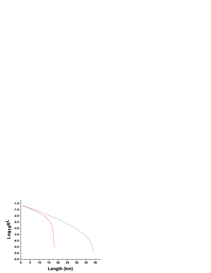
Figure 1: Lower bound of secret bit generation rate ($R_{1}^{L}$) verse fiber length $L$. Solid curve: no decoy states is employed, Alice just emits PDCS with half average number of photon pair $\lambda=0.1$. Dashed curve: for the 3-intensity case, Alice randomly used PDCS with half average number of photon pair $\lambda=0.1$, $\lambda^{\prime}=0.01$ and 0.

The $e_{1}^{U}$ is then calculated by equation (14). With this method, $R^{L}$ is obtained by equation (7). From Fig. 1, we found that the 3-intensity decoy states method can improve the performance of Boileau’s scheme dramatically. The longest security distance in original Boileau’s scheme is about 18 km while this distance for 3-intensity decoy states method will be 40 km. This improvement means about the 4.4dB increase in longest security distance.

V Conclusion

According to above discussions, we proved that through the introduction of decoy states method, especially the 3-intensity decoy states, the performance of Boileau’s DFS type QKD would be dramatically improved. Thanks to 3-intensity decoy state protocol the increase of longest security distance can be 4.4dB. This increase relays on the ability of 3-intensity decoy states protocol can obtain a tighter bound of $S_{1}^{L}$ and $e_{1}^{U}$. Furthermore one can estimate the information leaked to Eve with high precision and higher key bit rate and longer security distance can be obtained. We hope that our protocol could be implemented soon.

This work was supported by National Fundamental Research Program of China (2006CB921900), National Natural Science Foundation of China (60537020, 60621064) and the Innovation Funds of Chinese Academy of Sciences. To whom correspondence should be addressed, Email: zwzhou@ustc.edu.cn and zfhan@ustc.edu.cn.

References

- (1) C. H. Bennett, G.Brassard, Proceedings of IEEE International Conference on Computers, Systems, and Signal Processing, (IEEE, 1984), pp. 175-179.
- (2) A. K. Ekert, Phys. Rev. Lett. 67, 661 (1991)
- (3) N. Gisin et al., Rev. Mod. Phys. 74, 145 (2002)
- (4) Z. D. Walton, A. F. Abouraddy, A.V. Sergienko, B. E. A. Saleh, and M.C. Teich, Phys. Rev. Lett. 91, 087901 (2003)
- (5) J.-C. Boileau, R. Laflamme, M. Laforest, and C. R. Myers, Phys. Rev. Lett. 93, 220501 (2004)
- (6) Teng-Yun Chen, Jun Zhang, J.-C. Boileau, Xian-Min Jin, Bin Yang, Qiang Zhang, Tao Yang, R. Laflamme, and Jian-Wei Pan, Phys. Rev. Lett. 96, 150504 (2006)
- (7) M. Bourennane et al., Opt. Express 4, 383 (1999)
- (8) D. Stucki et al., New. J. Physics, 4, 41, (2002)
- (9) H. Kosaka et al., Electron. Lett. 39, 1199 (2003)
- (10) C. Gobby, Z.L. Yuan, and A.J. Shields, Appl. Phys. Lett. 84, 3762 (2004);
- (11) X.-F. Mo et al., Optics Letters, Vol. 30, Issue 19, pp. 2632-2634 (October 2005)
- (12) B. Huttner, N. Imoto, N. Gisin, and T. Mor, Phys. Rev. A 51, 1863 (1995);
- (13) G. Brassard et al., Phys. Rev. Lett. 85, 1330 (2000).
- (14) N. Lu tkenhaus, Phys. Rev. A 61, 052304 (2000).
- (15) W.-Y. Hwang, Phys. Rev. Lett. 91, 057901 (2003).
- (16) H.-K. Lo, X. Ma, and K. Chen, Phys. Rev. Lett. 94, 230504 (2005).
- (17) X.-B. Wang, Phys. Rev. Lett. 94, 230503 (2005);
- (18) X. Ma et al., Phys. Rev. A 72, 012326 (2005).
- (19) Y. Zhao et al., Phys. Rev. Lett. 96, 070502 (2006)
- (20) Yi Zhao et al, Proceedings of IEEE International Symposium on Information Theory 2006, pp. 2094-2098
- (21) C.-Z. Peng et al., Phys. Rev. Lett. 98, 010505 (2007)
- (22) D. Rosenberg, J. W. Harrington, P. R. Rice, et al., Phys. Rev. Lett. 98, 010503 (2007)
- (23) Z. L. Yuan, A. W. Sharpe, and A. J. Shields, Appl. Phys. Lett. 90 011118 (2007)
- (24) Tobias Schmitt-Manderbach et al., Phys. Rev. Lett. 98, 010504 (2007)
- (25) Z.-Q. Yin et al., quant-ph/0704.2941 (2007)
- (26) X.-B. Wang, Phys. Rev. A 72, 012322 (2005)
- (27) J.-B. Li, and X.-M. Fang, Chin. Phys. Lett. 23, No. 4 (2006)
- (28) Qing-yu Cai, and Yong-gang Tan, Phys. Rev. A. 73, 032305 (2006)
- (29) Tomoyuki Horikiri, and Takayoshi Kobayashi, Phys. Rev. A 73, 032331 (2006)
- (30) Qin Wang, X.-B. Wang, and G.-C. Guo, Phys. Rev. A 75, 012312 (2007)
- (31) Z.-Q. Yin, Z.-F. Han, F.-W. Sun, and G.-C. Guo, Phys. Rev. A 76, 014304 (2007)
- (32) Xiongfeng Ma, Chi-Hang Fred Fung, and Hoi-Kwong Lo, Phys. Rev. A 76, 012307 (2007)
- (33) D. Gottesman, H.-K. Lo, N. Lütkenhaus, and J. Preskill, Quantum Inf. Comput. 4, 325 (2004).
- (34) X.-B. Wang, C.-Z. Peng, and J.-W. Pan, Appl. Phys. Lett. 90, 031110 (2007)
- (35) X.-B. Wang, Phys. Rev. A 75, 052301 (2007)
- (36) Hoi-Kwong Lo and John Preskill, arXiv:quant-ph/0504209 (2005)