Experimental signatures of non-Abelian statistics in clustered quantum Hall states

Abstract

We discuss transport experiments for various non-Abelian quantum Hall states, including the Read-Rezayi series and a paired spin singlet state. We analyze the signatures of the unique characters of these states on Coulomb blockaded transport through large quantum dots. We show that the non-Abelian nature of the states manifests itself through modulations in the spacings between Coulomb blockade peaks as a function of the area of the dot. Even though the current flows only along the edge, these modulations vary with the number of quasiholes that are localized in the bulk of the dot. We discuss the effect of relaxation of edge states on the predicted Coulomb blockade patterns, and show that it may suppress the dependence on the number of bulk quasiholes. We predict the form of the lowest order interference term in a Fabry-Perot interferometer for the spin singlet state. The result indicates that this interference term is suppressed for certain values of the quantum numbers of the collective state of the bulk quasiholes, in agreement with previous findings for other clustered states belonging to the Read-Rezayi series.

I introduction

Probing exotic quantum statistics of particles is a long standing experimental challenge. In fractional quantum Hall effect systems, elementary excitations are expected to follow fractional statistics. There, it is difficult to experimentally distinguish the effects of Abelian fractional statistics from the effects associated with the fractional charge attributed to the same excitations. However, for states in which the statistics is expected to be non-Abelian, it is predicted that once the correct signature of this property is identified and measured, there will be no ambiguity in associating it with quantum statistics. For this reason alone, it is worth making the effort to explore the implication of non-Abelian statistics on measurable quantities.

Non-Abelian statistics is a key ingredient in the design of quantum gates for topologically protected qubits Kitaev (2003); Sarma et al. (2005); Nayak et al. (2008); Stern (2008). Experimental proof of the existence of non-Abelian anyons would be a major step towards an implementation of topological quantum computation.

Most suggested experiments aimed at probing non-Abelian statistics in quantum Hall systems consider a system designed to form a two path interferometer. The path difference between two quasiparticle (or quasihole) trajectories along the edge of the system forms a closed loop around a part of the system. The electronic density is determined by the positive background charge density and does not vary with magnetic field. Hence, a small deviation in the external applied magnetic field, introduces quasiparticles or quasiholes (depending on whether the magnetic field is increased or decreased), localized by impurities, into the loop Fradkin et al. (1998); Stern and Halperin (2006); Bonderson et al. (2006a, b); Chung and Stone (2006). As the number of these quasiparticles/quasiholes, $n$, is varied, the two terminal conductance is found to show a strong $n$-dependence via an interference term. Other experimentsStern and Halperin (2006); Ilan et al. (2008) considered tunneling of electrons into a large quantum dot whose interior is in a gapped quantum Hall state, and predicted how the clustering property of the Read-Rezayi (RR) states should influence Coulomb blockade peaks.

In this paper we have two goals. First, we extend the discussion of transport through dots in quantum Hall states belonging to the Read-Rezayi series and characterized by Coulomb blockade; we particularly address the issue of the different time scales involved in the experiment. The fastest time scale is the time in which a current carrying electron traverses the dot, $e/I$. For these electrons the bulk of the dot is inaccessible, and they occupy the lowest energy state on the edge. A much slower time scale is that in which the area of the dot is varied. If this scale is slow enough, the electrons that are added to the dot when its area is varied may make use of bulk states. We assume, for concreteness, that the magnetic field is tuned such that there are quasiholes localized in the bulk, rather than quasiparticles. The internal bulk states are then carried by these localized quasiholes. For that to happen, however, weak coupling should exist between the bulk quasiholes and the edges.

In previous discussions of Coulomb blockade measurements in such an experimentStern and Halperin (2006); Ilan et al. (2008), the hidden assumption was that as the variation of the area adds electrons to the dot, these added electrons make use only of states at the edge. In the language of topological field theory (TFT), the fusion channel of all the quasihole operators in the bulk of the dot is fixed at the beginning of the experiment, and does not change as new electrons are added to the dot. In the present paper we consider the possibility that as the area is slowly varied, weak coupling of the bulk and the edge may allow for the fusion channel to change when electrons are added, in such a way that energy is minimized.

Second, we analyze the Fabry-Perot setting in another non-Abelian quantum Hall state, a $\nu=4/7$ spin-singlet state, whose experimental signatures have not been considered so far. This state was suggested by Ardonne and SchoutensArdonne and Schoutens (1999). It is the first in a series of spin-singlet states with order-$k$ clustering, at filling fraction $\nu=\frac{2k}{2k+3}$. The $k>1$ states support spinful quasihole excitations with non-Abelian statistics. For the paired ($k=2$) state at $\nu=4/7$ the quasiholes are Fibonacci anyons Ardonne and Schoutens (2007). Experimentally, a spin transition for quantum Hall states around $\nu=4/7$ has been observed in samples with reduced Zeeman splitting Cho et al. (1998), but this feature may also indicate an unpolarized Abelian state of the Jain series. Transport properties we analyze here may distinguish between the two candidate states. The fact that possible fractional quantum Hall states in graphene are expected to be spin-singlet with respect to the pseudo-spin (valley) index Tőke et al. (2006), provides additional motivation for studying non-Abelian statistics for spin-singlet states. In this paper we study Coulomb blockade transport through a dot in the $\nu=4/7$ non-Abelian spin-singlet state, with and without relaxation. We also analyze the lowest order interference in a Fabry-Perot interferometer and derive a characteristic suppression factor.

The paper is organized as follows. In Sec. II, we discuss the experimental setup in which these experiments are to be carried out. In Sec. III we discuss in short the general structure of the conformal field theories (CFT) describing these states. In Sec. IV we discuss in detail the formation of Coulomb blockade peaks in the conductance through large quantum dots in the RR states. In Sec. V we turn to implement the same ideas to the spin singlet state in order to predict the result for the Coulomb blockade peaks. We also calculate the interference term of the current in a two path interferometer for this state.

II General considerations

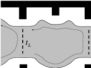
Figure 1: Setup for an interference experiment. The gray region is a gapped quantum Hall fluid. Two possible tunneling paths for an incoming edge quasihole are marked. There are $n$ quasiholes localized in the area between the two quantum point contacts.

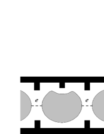
Figure 2: Fabry Perot interferometer in the limit of strong quasihole backscattering. Transport through the dot is done via electron ($e$) tunneling. The area $S$ of the dot may be varied using a side modulation gate.

The Fabry-Perot interferometer, sketched in Fig. 1, is a Hall bar with two quantum point contacts (QPCs) introducing quasiparticle/quasihole tunneling from one edge to the other. We deal with two opposite limits of this interferometer: weak inter-edge back-scattering, in which we look at interference to lowest order, and strong inter-edge backscattering, where the interferometer becomes a quantum dot, whose Coulomb blockade peaks we study.

As mentioned above, we shall always assume that there are quasiholes, rather than quasiparticles, that are localized in the bulk. For the purpose of lowest order interference calculations, when one is also required to consider excitations on the edge, we shall consider for convenience that the current along the edge is also carried by quasiholes. Changing this current to be of quasiparticles should not modify our results.

Lowest order interference is observed when a single quasihole does not tunnel between opposite edges more than once. The tunneling process introduces a finite value for the longitudinal conductance. The measured backscattered current, injected from the left along the lower edge and collected on the left at the upper edge, interferes only through two trajectories: quasiholes entering from the left along the lower edge are either being backscattered at the left QPC, or transmitted at the left QPC and reflected from the right one. The path difference between the two trajectories forms a closed loop around the island confined between the contacts, which may contain localized quasiholes in the bulk of the sample. For the sake of discussing lowest order interference, we assume that there is no hopping of quasiholes between the bulk and the edge.

The two trajectories sketched in Fig. 1 are associated with two partial waves, $|\Psi_{L}\rangle$ and $|\Psi_{R}\rangle$. While these partial waves differ by global phases originating from the total magnetic field through the island (due to the Aharonov-Bohm effect), their overlap also encodes information on the mutual statistics of the quasiholes in the system. As mentioned in sec. I, this is attributed to the fact that the path difference between the two trajectories of the edge qusiholes forms a closed loop encircling localized quasiholes. Altogether, the back-scattered current will be of the form

$$I_{bs}\propto|t_{L}|^{2}+|t_{R}|^{2}+2\,\text{Re}\left\{t_{L}^{*}t_{R}\langle\psi_{L}|\psi_{R}\rangle\right\}.$$ (1)

It is the overlap $\langle\psi_{L}|\psi_{R}\rangle$ that we calculate below.

In the limit of strong back-scattering (Fig. 2), when the two point contacts on either side of the island are almost closed, the number of electrons in the dot confined between them is quantized to an integer. Quasihole or quasiparticle tunneling into and out of this region is forbidden, and the only way to transport charge through it is by tunneling of electrons. Low-voltage low-temperature conductance through the dot is suppressed due to charging energy, except at ”Coulomb blockade peaks”, when the ground state energy of the dot with $N_{e}$ electrons is degenerate with its ground state energy with $N_{e}+1$ electrons. Coulomb blockade peaks may be probed by measuring the conductance through the dot as a function of a magnetic field $B$ and the dot’s area $S$, since a variation of $S$ with fixed $N_{e}$ violates charge neutrality with the positive background Ilan et al. (2008). Peaks in the conductance appear for those values of the area $S$ and magnetic field $B$, for which the following equation

$$E(N_{e},S,B)=E(N_{e}+1,S,B)$$ (2)

is satisfied for some integer $N_{e}$ representing the total number of electrons inside the dot.

The quantum Hall liquid is largely gapped, with two exceptions: the edge and the internal degrees of freedom of the bulk quasiholes. As we will review below, the state of the internal degrees of freedom of the bulk quasiholes determines the spectrum of the edge, that determines, in turn, the position of the Coulomb peaks.

In Ref. (Ilan et al., 2008), Coulomb blockade peaks were mapped for large dots in a quantum Hall state of the RR series $\nu=\frac{k}{k+2}$, under the assumption that the state of the bulk quasiholes is frozen. For a clean large ($N_{e}\gg 1$) dot in a metallic state at zero magnetic field, and dots in the integer and Abelian fractional quantum Hall states the area spacings between consecutive Coulomb blockade peaks is $\Delta S=e/n_{0}$, the area occupied by one electron. In contrast, for the RR series the Coulomb blockade peaks location as a function of the area at a fixed magnetic field (i.e., a fixed number of localized bulk quasiholes $n$) was found to depend on $B$. While the average spacing between peaks remains $e/n_{0}$, the presence of non-Abelian quasiholes in the bulk causes the peaks to bunch into groups, where the number of peaks in each group depends on $k$ and on $n$.

The edge energies of the non-Abelian quantum Hall states we discuss in this paper are stored in a bosonic charged edge mode (a chiral Luttinger liquid) and one or several neutral edge modes. With $N_{e}=0$ defined to be the number of electrons for a dot with area $S_{0}$, the energy associated with the charge mode for $N_{e}$ electrons on the edge is Ilan et al. (2008)

$$E_{c}(N_{e})=\frac{\pi v_{c}}{\nu L}\left(N_{e}-\nu\frac{B_{0}(S-S_{0})}{\phi_{0}}\right)^{2}.$$ (3)

where $\phi_{0}$ is the magnetic flux quantum. The magnetic field $B=B_{0}$ is that in which there are no quasiholes in the bulk, $\nu$ is the filling fraction of the partially filled topmost Landau level, $v_{c}$ is the velocity of the charged edge mode, and $L$ is the perimeter of the quantum dot (we take $\hbar=1$). For Abelian Laughlin states, where there is only a single bosonic mode, Eq. (2) reduces to $E_{c}(N_{e})=E_{c}(N_{e}+1)$, and the area separation $\Delta S$ between its solutions for consecutive values of $N_{e}$ is $\Delta S=e/n_{0}$, where $n_{0}$ is the charge density inside the dot. The value of $\Delta S$ in this case is independent of the magnetic field. For non-Abelian states, this is not the case. Below, we focus on the contribution of the neutral mode, and add the charge contribution Eq. (3) at the final stage.

The assumptions underlying the calculation performed in Ref. (Ilan et al., 2008) were that the magnetic field, and therefore the number of quasiholes, is fixed at the beginning of the experiment, and that the dot is relaxed into its ground state. It was also assumed that the initial number of electrons inside the dot was divisible by $k$, such that all electrons are clustered in the bulk of the dot and the occupation of the electron states of the edge is zero. Then, with a fixed number of quasiholes in the bulk, the area is varied fast enough such that there is no time for the electrons to relax onto states with lower energies that may be available.

Here, we allow the initial number of electrons to have any integer value. For concreteness we assume that the dot has no bulk quasiholes in the beginning of the experiment. The number of electrons then dictates the number of edge modes that are initially occupied. Shifting the magnetic field creates a fixed number of quasiholes in the bulk, whose fusion channel is determined by energetic considerations we explain in details later on. The process of introducing quasiholes into the bulk is done slowly enough for the edge and the bulk to equilibrate. Finally, once the number of quasiholes and their fusion channel is determined, we move on to consider what happens when the area of the dot is varied.

In our analysis we consider the implications of varying the area slowly enough such that the state of the bulk quasiholes may changes adiabatically. As the area of the dot grows, more electrons are added to the dot. In the absence of edge-bulk coupling, the state of the bulk quasiholes does not change, and the added electrons affect only the state of the edge. With bulk-edge coupling, tunneling of neutral modes between the edge and the bulk quasiholes may change the state of the bulk quasiholes.

We may envision both elastic and inelastic bulk-edge couplings. In the former, a tunnel coupling allows for the hopping of a neutral particle (whose properties are to be described belowRosenow et al. (2008); Overbosch and Wen (2007)) between the bulk and the edge. In the latter, this hopping is accompanied by an energy transfer to an outside thermal bath, e.g., by an emission of a phonon. The latter is thus also an irreversible relaxation mechanism that allows the system to cool. Quantitative estimate of these two types of couplings are not possible at our present level of understanding of the microscopy of the samples and the involved quantum Hall states. Both are, however, bound to exist to some level. In this work we study in details the process involving energy relaxation. We also discuss qualitatively the effect of the first process for the particular case of $\nu=5/2$.

The following argument may illuminate the way the state of the bulk quasiholes affects the spectrum of the edge: consider a sphere in a RR state with $N_{e}$ electrons that are all clustered in clusters of $k$ electrons. Assume the sphere has $n$ quasiparticles and $n$ quasiholes, which are localized by impurities away from one another. The ground state is then degenerate, with the degeneracy being exponential in $n$ (for large $n$). Topologically, each quasiparticle/quasihole is equivalent to a puncture in the sphere. Now imagine bringing the $n$ quasiparticles close together, i.e., fusing together $n$ of the holes pierced in the sphere. The proximity of the quasiparticles to one another lifts the degeneracy, and the way it is lifted is determined by the state to which the $n$ quasiparticles fuse. This system is topologically equivalent to the system we are interested in, a disk that has $n$ quasiholes localized in its bulk.

The energies appearing on both sides of Eq. (2) belong to the spectrum of the edge theory. The main challenge in obtaining the spectrum for non-Abelian states is to construct the part of it that follows from the addition of a parafermion theory to that of the chiral boson contributing the charging energy Eq. (3). In the next section, we describe briefly and most generally what is the relation between parafermionic field theories and the quantum Hall effect, and who are the main players in these theories. When discussing a particular quantum Hall state, either one that belongs to the RR series or the spin singlet state, we will first specialize the discussion to the parafermionic CFT relevant to it and review its properties. We will single out the parafermion used to construct the electron operator, and explain how the construction of the Hilbert space is done and the spectrum is found. Dwelling on the details of the parafermionic CFT is also crucial in order to understand the calculation of the interference term of Eq. (1), as some of the phases of the two partial waves interfering are contributed by fields in this parafermionic theory.

III The CFT description of quantum Hall states

Conformal field theories (CFTs) are used in several different contexts regarding quantum Hall systems. Trial many-body wavefunctions for single Landau level fractional quantum Hall states are created from CFTs (in $D=2+0$ dimensions) as correlators of fields representing different particles in the system Moore and Read (1991); Read and Rezayi (1999); Ardonne and Schoutens (2007); Hansson et al. (2007). Starting from chiral boson theories, one constructs Abelian fractional quantum Hall wavefunctions such as those in the Laughlin series. Including parafermionic field theories leads to wavefunctions for non-Abelian quantum Hall states. While explicit closed form expressions are available for RR states for general $k$ (see Refs. (Ardonne and Schoutens, 2007; Cappelli et al., 2001; Read and Rezayi, 1999)), not all physical properties are easily explored on the basis of these wavefunctions alone. Excitations at the edge of a quantum Hall droplet are described by the same CFTs, now viewed in $D=1+1$ dimensions.

A theoretical construction of the paired quantum Hall state at filling factor $1/2$ was originally proposed in the context of CFT, and is easily understood in that language Moore and Read (1991). The theoretical construction of a wavefunction for this state involves the $\mathbb{Z}_{2}$ theory, also known as the Ising CFT. The use of this CFT yields the Pffafian wavefunction, implying that the gapped state of the bulk is similar to that of a $p_{x}+ip_{y}$ superconductor in the weak pairing phaseRead and Green (2000). Therefore, this state is thought of as a superconductor, a condensate of Cooper-pairs of composite-fermions.

The field taken from the $\mathbb{Z}_{2}$ theory and used to define the electron operator for the $1/2$ state is a neutral fermion, and in fact represents the composite fermion. For members of the RR series with a higher value of $k$, this composite fermion is replaced by a composite anyon, and the operator taken from the $\mathbb{Z}_{k}$ theory is called a parafermion (which no longer obeys fermionic statistics). In that case, the gapped state of the bulk is thought of as a condensation of clusters of such anyons. The size of the clusters is determined by the minimal number of such parafermions which may be combined into an effective boson, which then Bose-condense. For the $\mathbb{Z}_{k}$ theory this number is $k$. The equivalent statement in the language of CFT is that a parafermionic CFT at level $k$ can be used to describe a state in which $k$ electrons form a cluster. This is because the fusion rules of this parafermion theory always imply that $k$ copies of the fundamental field used to define the electron operator fuse to the identity operator.

Since they were first theoretically constructed using parafermion CFTs, these same CFTs remained the main available theoretical tool to explore various properties of quantum Hall clustered states other than the Moore-Read state. While the Moore-Read state may be conveniently explored using the theory of superconductivity, no analogous description exists for other clustered states.

A general parafermionic theoryGepner (1987) is a coset model $G_{k}/U(1)^{\ell}$, where $G_{k}$ is a simple affine Lie algebra of rank $\ell$. The fields are labeled $\Phi^{\Lambda}_{\lambda}$, where both $\Lambda$ and $\lambda$ are weights of the simple Lie algebra $G$. These fields are subject to some restrictions and identifications, and we will specify them when dealing with a specific parafermion theory below. The conformal dimension of these fields is given by

$$h_{\lambda}^{\Lambda}=\frac{\Lambda\cdot(\Lambda+2\rho)}{2(k+g)}-\frac{\lambda\cdot\lambda}{2k}+n^{\Lambda}_{\lambda}$$ (4)

where $2\rho$ is the sum of the positive roots of the Lie algebra $G$, and the scalar product $(\cdot)$ is with respect to the quadratic form matrix (for more details see Ref. (DiFrancesco et al., 1997)). The integer $n^{\Lambda}_{\lambda}$ is equal to the grade of the representation of the current algebra in which $\Phi_{\lambda}^{\Lambda}$ appearsGepner (1987).

The parafermion field is denoted by $\psi_{\alpha}$, and belongs to the set of fields $\Phi_{\alpha}^{0}$, where $\alpha$ is a root, and the vector $0$ is the vacuum representation. The OPE of a parafermion and a field $\Phi^{\Lambda}_{\lambda}$ is given by

$$\psi_{\alpha}(z)\Phi^{\Lambda}_{\lambda}(0)=\sum_{m=-\infty}^{\infty}z^{-\alpha\cdot\lambda/k-1-m}[A^{\alpha,\lambda}_{m}\Phi^{\Lambda}_{\lambda}](0)$$ (5)

Note that the product of roots $\alpha\cdot\lambda$ is with respect to the quadratic form matrix. The modes $A^{\alpha}_{m}$ obey generalized commutation relations.

IV Read-Rezayi states and $\mathbb{Z}_{k}$ parafermions

Consider a 2DEG experiencing one of the plateaus belonging to the RR series. When the magnetic field is varied by one flux quantum, $k$ quasiholes appear, hence the flux associated with a single quasihole is $\frac{\phi_{0}}{k}$. Combined with the fact that the filling factor is $k/(k+2)$, this implies that quasiholes for RR states have charge $\frac{e}{k+2}$ .In order to fully describe the edge of the RR state, one must add a second field theory to that of the chiral boson, a CFT known as $\mathbb{Z}_{k}$ parafermions Zamolodchikov and Fateev (1985); Gepner and Qiu (1987). In this theory the algebra $G_{k}$ is $SU(2)_{k}$ of rank $\ell=1$, and therefore the theory is equivalent to the coset model $SU(2)_{k}/U(1)$.

The fields in the theory are labeled by two quantum numbers $\Phi^{l}_{m}$, with $l\in\left\{0,1,\ldots,k\right\}$. The integer $m$ is known as the $\mathbb{Z}_{k}$ charge of the field $\Phi_{m}^{l}$ and is defined modulo $2k$. The fields are subjected to the following identifications $\Phi_{m}^{l}=\Phi_{m+2k}^{l}=\Phi_{m-k}^{k-l}$ and $l+m=0\bmod 2$.

The creation operators of both electrons and quasiholes in the bulk are products of two factors. The first is a vertex operator, $e^{i\alpha\varphi(z)}$, that accounts for the flux and the charge associated with the electron ($\alpha=\sqrt{(k+2)/k}$), and with the quasihole ($\alpha=1/\sqrt{k(k+2)}$) (this vertex operator is sufficient for the description of Abelian statesWen (1992)). The second factor is one of the fields in the parafermionic theory; the electron creation operator is given by $\psi_{1}e^{i\sqrt{\frac{k+2}{k}}{\varphi}}$, where $\psi_{1}=\Phi_{2}^{0}$ is one of the parafermionic currents, while the quasihole creation operator is $\sigma_{1}e^{i\sqrt{\frac{1}{k(k+2)}}{\varphi}}$, where $\sigma_{1}$ is one of the parafermionic primary fields (see below).

The parafermion $\psi_{1}$ has the following operator product expansion with a field of $\mathbb{Z}_{k}$ charge $q$

$$\psi_{1}(z)\Phi_{q}(0)=\sum_{p=-\infty}^{\infty}z^{-p-1-q/k}A_{(1+q)/k+p}\Phi_{q}(0).$$ (6)

The fields $A_{(1+q)/k+p}\Phi_{q}(0)$ have $\mathbb{Z}_{k}$ charge $q+2$. Similarly, the mode expansion of the parafermion $\psi_{1}^{\dagger}=\psi_{k-1}$ is given by

$$\psi^{\dagger}_{1}(z)\Phi_{q}(0)=\sum_{p=-\infty}^{\infty}z^{-p-1-q/k}A^{\dagger}_{(1-q)/k+p}\Phi_{q}(0).$$ (7)

and the field $A^{\dagger}_{(1-q)/k+p}\Phi_{q}(0)$ has $\mathbb{Z}_{k}$ charge $q-2$.

The different modes of the field $\psi_{1}$,

$$A_{(1+q)/k+p}=\frac{1}{2\pi i}\oint dz\psi_{1}(z)z^{q/k+p},$$ (8)

obey generalized commutation relations, that may be found by evaluating the integral

$$\frac{1}{(2\pi i)^{2}}\left[\oint_{0}dz,\oint_{0}dw\right]\psi_{1}(z)z^{q/k+\mu}\,\psi_{1}(w)w^{q/k+\nu}(z-w)^{2/k},$$

where $\mu$ and $\nu$ are integers. These commutation relations take the form

$$\sum_{\ell\geq 0}c^{(\ell)} \left[A_{(3+q)/k+\mu-\ell}A_{(1+q)/k+\nu+\ell}\right.$$ (9)

$$\left.-A_{(3+q)/k+\nu-\ell}A_{(1+q)/k+\mu+\ell}\right]=0$$

(when acting on a field with charge $q$), where $c^{(\ell)}=\Gamma(\ell-2/k)/\ell!\Gamma(-2/k)$. The same method can be used to obtain expressions for the generalized commutation relation between the different modes $A^{\dagger}$ of $\psi_{1}^{\dagger}$, and between the $A^{\dagger}$s and $A$sZamolodchikov and Fateev (1985); Gepner and Qiu (1987).

The parafermionic primary fields $\Phi_{l}^{l}$ are defined by the condition

$$A_{(1+\ell)/k+p}\Phi_{l}^{l}=A^{\dagger}_{(1-\ell)/k+p+1}\Phi_{l}^{l}=0\quad\text{for}\ p\geq 0$$ (10)

The primary fields are usually denoted $\sigma_{l}$ and referred to as spin fields. Their conformal dimension is given by

$$h_{l}=\frac{l(k-l)}{2k(k+2)}.$$ (11)

Each of these fields generates a series of fields $\Phi_{m}^{l}$ by applications of the modes $A$ of the parafermion $\psi_{1}$, and the modes $A^{\dagger}$ of the parafermion $\psi_{1}^{\dagger}$. The conformal dimension of the field $\Phi_{m}^{l}$ is given by

$$h^{l}_{m}=h_{l}+\frac{(l-m)(l+m)}{4k},\ \text{for}\ -l<m\leq l\quad$$

$$h^{l}_{m}=h_{l}+\frac{(m-l)(2k-l-m)}{4k},\ \text{for}\ l<m\leq 2k-l\quad\quad\ .$$ (12)

The fusion rules for the parafermionic CFT are Zamolodchikov and Fateev (1985); Gepner and Qiu (1987)

$$\Phi_{m_{\alpha}}^{l_{\alpha}}\times\Phi_{m_{\beta}}^{l_{\beta}}=\sum\limits_{l_{\gamma}=\left|l_{\alpha}-l_{\beta}\right|}^{\min\left\{l_{\alpha}+l_{\beta},2k-l_{\alpha}-l_{\beta}\right\}}\Phi_{m_{\alpha}+m_{\beta}}^{l_{\gamma}}.$$ (13)

The operator product expansion (OPE) is given by

$$\Phi_{m_{\alpha}}^{l_{\alpha}}(z)\Phi_{m_{\beta}}^{l_{\beta}}(w)=\sum_{l_{\gamma}}C_{\alpha\beta\gamma}(z-w)^{\Delta h}\ \Phi_{m_{\alpha}+m_{\beta}}^{l_{\gamma}}(w)$$ (14)

where the fields appearing on the right hand side are determined by Eq. (13), $C_{\alpha\beta\gamma}$’s are constants, and $\Delta h=h_{m_{\alpha}+m_{\beta}}^{l_{\gamma}}-h_{m_{\beta}}^{l_{\beta}}-h_{m_{\alpha}}^{l_{\alpha}}$. As a consequence of that relation, when a field $\Phi_{m_{\alpha}}^{l_{\alpha}}$ goes around a field $\Phi_{m_{\beta}}^{l_{\beta}}$ and their fusion is to a field $\Phi_{m_{\alpha}+m_{\beta}}^{l_{\gamma}}$, the phase generated is $2\pi\Delta h$.

IV.1 Coulomb blockade for Read-Rezayi states

To determine the parafermionic part of the ground state energy for a dot with electrons on the edge, we need to construct a basis of states for the parafermion theory and extract from it the lowest-lying energy state with $0\leq j<k$ parafermions. Such a basis was constructed using the modes of the fundamental parafermion $\psi_{1}$ in Ref. (Jacob and Mathieu, 2002), see also Ref. (Schoutens, 1997; Bouwknegt and Schoutens, 1999), and used in Ref. (Ilan et al., 2008). A general state with $j$ parafermions of the type $\psi_{1}$ is of the form

$$A_{-p_{j}+(2j+q-1)/k}A_{-p_{j-1}+(2j+q-3)/k}\cdot\cdot\cdot A_{-p_{1}+(1+q)/k}|\sigma_{q}\rangle,$$ (15)

where the $p_{i}$ are integers, and $|\sigma_{0}\rangle=|0\rangle$. This state is an eigenstate of the Hamiltonian with energy

$$E(j,q) =h_{q}-\sum_{i=0}^{j-1}\frac{q+1+2i}{k}+\sum_{i=1}^{j}p_{i}$$ (16)

$$=h_{q}-\frac{j(j+q)}{k}+\sum_{i=1}^{j}p_{i}$$

in units of $\frac{2\pi v_{n}}{L}$, where $v_{n}$ is the velocity of the neutral modes as they propagate along the edge. Since we are looking for the lowest-energy state, the integers $p_{i}$ are chosen such that the state has the lowest possible energy, and is not a null state. The conditions are that $p_{i}=1$ for $i\leq k-q$ and $p_{i}=2$ for $i>k-q$. In order to obtain these conditions one has to use the generalized commutation relations given in equation (9), see Ref. (Jacob and Mathieu, 2002) for details. The lowest energy for a given value of $j$ and $q$ is therefore given by

$$E_{\psi}(j,q)=h_{q}+\left\{\begin{array}[]{ccc}\frac{j(k-j-q)}{k}&\qquad{\rm for}&j\leq k-q\\ \\ \frac{(k-j)(j+q-k)}{k}&\qquad{\rm for}&j>k-q\\ \end{array}\right.$$ (20)

It is easy to see that for a particular value of $q$ and $j$, the energy is simply the conformal dimension of the field which is the result of the fusion product of $\sigma_{q}$ and $j$ copies of the parafermion $\psi_{1}$. Also, since

$$\Phi^{q}_{q+2j}=A_{-1+(2j+q-1)/k}A_{-1+(2j+q-3)/k}\cdot\cdot\cdot A_{-1+(1+q)/k}\Phi_{q}^{q},$$ (21)

for $j=k-q$ the energy $E_{\psi}(k-q,q)=h_{q}$ , i.e, the same as the conformal dimension of the highest weight state. This is because $\Phi^{q}_{q+2(k-q)}=\Phi^{k-q}_{k-q}=\sigma_{k-q}$, and the conformal dimension of the spin field, Eq. (11), is invariant under the substitution $l\rightarrow k-l$.

We now turn to a description of the experimental procedure. First, we characterize the state of the dot containing a quantum Hall droplet at the beginning of the experiment, when the magnetic field is set to some constant value, the number of electrons has some quantized value, the area of the dot is fixed and the dot is relaxed to its ground state.

For the edge of a quantum Hall system, the charge $q$ of the highest weight state of the edge theory is determined by the number of quasiholes in the bulk and the total number of electrons in the dot, as we show below. Whether or not it stays fixed throughout the experiment (as the area is varied), depends on the rate at which the area is varied. This issue and its influence on the outcome of the experiment will be discussed at later stage.

Let us start with a dot where the number of electrons is divisible by $k$. By setting the magnetic field to a certain value for which the filling factor is a bit less than $k/(k+2)$, quasiholes may be introduced into the bulk, while their counterparts of opposite charge and topological charge are introduced onto the edge. The contribution of the charged part of the edge quasiparticles influences the boundary conditions of the chiral boson theoryIlan et al. (2008). The parafermionic part of the edge will be taken from the fusion product of $n$ copies of the field $\sigma_{k-1}$, the spin field that makes the edge quasiparticles.

The bulk quasiholes may have several fusion channels as dictated by Eq. (13). According to the fusion channel $\Phi_{bulk}$ of the bulk quasiholes, i.e, of $n$ copies of the field $\sigma_{1}$, the fusion channel $\Phi_{edge}$ of the $n$ copies of $\sigma_{k-1}$ on the edge will be fixed by the requirement that $\Phi_{bulk}\times\Phi_{edge}\sim\mathbf{1}$, and by the requirement of energy minimization. We now explain how to determine which fusion channel will ultimately be selected.

For a particular value of the magnetic field, the number of localized quasiholes is fixed, and therefore the bulk has a single quantized value of $\mathbb{Z}_{k}$ charge which is equal to $n\bmod k$. This value of the $\mathbb{Z}_{k}$ charge may correspond to several fusion channels of the parafermionic part of the quasihole operators. Had the system with localized quasiholes been infinite with no edge, all fusion channels of the bulk quasiholes would be have been degenerate in energy. This is the essential ingredient which causes these quasiholes to have non-Abelian statisticsMoore and Read (1991); Read and Rezayi (1999). The presence of the edge and the excitations living on it will lift the degeneracy of these fusion channels. The reason is that while all possible fusion channels of a particular number of quasiholes have the same $\mathbb{Z}_{k}$ charge, different fusion channels correspond to different highest weight states with different initial occupation of parafermions on the edge, and therefore have different energies.

Let us consider for clarity the example of $\mathbb{Z}_{3}$ parafermions, assumed to describe the quantum Hall state at filling factor $\nu=12/5$. In this parafermionic theory there are two parafermions, $\Phi_{2}^{0}=\psi_{1}$ and $\Phi_{4}^{0}=\psi_{2}$, and two parafermionic primary fields, $\Phi_{1}^{1}=\sigma_{1}$ and $\Phi_{2}^{2}=\sigma_{2}$. We denote $\Phi_{3}^{1}=\Phi^{2}_{0}=\epsilon$. The possible $\mathbb{Z}_{k}$ charge of the bulk is $0,1$ or $2$.

Suppose that the number of quasiholes in the bulk is $3m+1$, where $m$ is some integer. Then, the possible fusion channels of these quasiholes are

$$(\sigma_{1})^{3m+1}\sim\psi_{2}+\sigma_{1}\ .$$ (22)

Accordingly, the two fusion channels of the edge are $\psi_{1}$ and $\sigma_{2}$. The two possible edge states in this case are therefore

$$A_{-2/3}|0\rangle,\quad|\sigma_{2}\rangle$$ (23)

with $E_{\psi}=2/3$ and $E_{\sigma}=1/15$ (in units of $2\pi v_{n}/L$) respectively. If the initial edge state of the dot is set by energy considerations, then the fusion channel of the bulk quasiholes will be $\sigma_{1}$. It is easy to check that if there are $3m+2$ quasiholes in the bulk, the fusion channel of the bulk will be $\sigma_{2}$, resulting in the lowest energy state $|\sigma_{1}\rangle$ on the edge.

For a general value of $k$, the lowest energy of the dot will be achieved when the edge has the lowest possible energy, under the restriction that the $\mathbb{Z}_{k}$ charge of the edge state is $k-\tilde{n}$ where we write $\tilde{n}\equiv[n]_{k}\equiv n\bmod k$. The unique edge state fulfilling this requirement is the highest weight state $|\sigma_{k-\tilde{n}}\rangle$. Therefore, the requirement that the dot is totally relaxed into its ground state, sets the fusion channel of the bulk quasiholes to be $\Phi_{bulk}=\sigma_{\tilde{n}}$.

If the initial number of electrons in the dot, $N_{e}$, is not divisible by $k$, and in the absence of bulk quasiholes, there will be a number $s$ of parafermion modes occupying edge states, and the lowest energy of the dot will depend also on $s$. In the background of a RR quantum Hall state, an additional electron is represented by a bulk operator carrying a parafermion field $\psi_{1}$. For the complete system to maintain zero topological charge, this implies the presence of a corresponding dual field, $\psi_{1}^{\dagger}=\psi_{k-1}$, on the edge. For a total of $N_{e}$ electrons, the edge $\mathbb{Z}_{k}$ charge will be $2[-N_{e}]_{k}$, as can be seen by adding the $\mathbb{Z}_{k}$ charges of the $\psi_{k-1}$ modes that come with every additional electron. Note that it is always possible to construct states using only modes of $\psi_{1}$, due to the relation $\psi_{1}^{\dagger}=\psi_{k-1}\sim(\psi_{1})^{k-1}$. For example, a state with a single occupied mode of $\psi_{1}^{\dagger}$ is equivalent to an edge state of the form (15) with $j=k-1$ occupied modes of $\psi_{1}$. Therefore, the number of occupied edge modes of the field $\psi_{1}$ will be $s=[-N_{e}]_{k}$.

As the magnetic field is slightly shifted, quasiholes are introduced into the bulk.The lowest possible energy of the edge will then be equal to the smallest conformal dimension of the field which is a result of the fusion product of $s$ parafermions of the type $\psi_{1}$ and $n$ copies of the field $\sigma_{k-1}$, with $n$ being the number of localized quasiholes. This lowest energy is then the smallest conformal dimension of a field with charge $[2s-n]_{k}$.

The lowest conformal dimension of a field with a given $\mathbb{Z}_{k}$ charge always belongs to the parafermionic primary field of that charge. Therefore, the lowest energy of a dot with $n$ bulk quasiholes and $s$ parafermions on the edge is $h_{[2s-n]_{k}}$. If the system is assumed to be initially relaxed into its absolute ground state then the fusion channel of the bulk will be such that all parafermionic fields on the edge will fuse to $\sigma_{[2s-n]_{k}}$.

Again, let us consider an example from $\mathbb{Z}_{3}$ parafermions. Suppose that the number of quasiholes in the bulk is $3m$, and the number of electrons in the dot is $3j+1$ where $j$ and $m$ are integers. The $\mathbb{Z}_{k}$ charge contributed to the edge due to the presence of the extra bulk electron is $2[-N_{e}]_{k}=4$ corresponding to the two fields $\sigma_{1}$ and $\psi_{2}$. Using this fact, we find that the two possible edge states are

$$A_{0}A_{-2/3}|0\rangle,|\sigma_{1}\rangle$$ (24)

with energy $E=2/3$ and $E=1/15$ respectively. Therefore, the second state is energetically favorable. Indeed we see that the lowest energy edge state is associated with the spin field of charge $[2s-n]_{k}=1$. The fusion channel of the $3m$ quasiholes in the bulk in this case will be set to $\epsilon$.

We conclude that the presence of a number of electrons in the dot which is not divisible by $k$ at the beginning of the experiment influences the fusion channel of the bulk quasiholes. It sets the highest weight state on which parafermionic modes act.

We now turn to consider the course of the experiment. Once the initial value of $q$ is set according to the initial occupation of modes on the edge and the number of bulk quasiholes, the area is varied. As an electron tunnels into the dot, the occupation of parafermion modes on the edge changes, but we assume that the electron does not couple to any bulk modes. While the initial state of the dot was a highest weight state with charge $q=[2s-n]_{k}$, and therefore had the lowest possible energy, bringing the next electron into the dot results in the edge state $A^{\dagger}_{(1-q)/k}|\sigma_{q}\rangle$ with charge $q-2$. This is not necessarily the state of lowest possible energy for this charge, since the lowest possible energy is the conformal dimension of $\sigma_{q-2}$, and $A^{\dagger}_{(1-q)/k}\sigma_{q}$ is not necessarily equal to $\sigma_{q-2}$.

For the system to relax into the ground state after a change in the area of the dot makes an electron tunnel into or out of the dot, it has to change the fusion channel of the bulk quasiholes, and the fusion channel of the $n$ copies of $\sigma_{k-1}$ on the edge. Since before the electron tunneled the fusion of the parafermionic fields on the edge was

$$(\psi_{1})^{s}(\sigma_{k-1})^{n}\sim\sigma_{[2s-n]_{k}},$$ (25)

and thus, that of the spin fields on the edge was

$$(\sigma_{k-1})^{n}\sim\Phi^{[2s-n]_{k}}_{[2s-n]_{k}-2s},$$

the lowest energy for an edge with one extra electron is obtained when

$$\psi_{k-1}(\psi_{1})^{s}(\sigma_{k-1})^{n}\sim(\psi_{1})^{s-1}(\sigma_{k-1})^{n}\sim\sigma_{[2(s-1)-n]_{k}},$$ (26)

i.e, the fusion channel of the spin fields on the edge should be

$$(\sigma_{k-1})^{n}\sim\Phi^{[2(s-1)-n]_{k}}_{[2(s-1)-n]_{k}+2(s-1)}.$$

Here, we assumed that the relaxation of the edge has to take place only through a change in the fusion channel of the quasiholes. This assumption amounts to assuming that no excitation with non-trivial $\mathbb{Z}_{k}$ charge can tunnel between the bulk and the edge. This point will be further discussed in Sec.  IV.1.2.

Whether the fusion channel of the spin fields on the edge (and therefore of the quasiholes in the bulk) changes every time the change in the dot’s area leads to a change in the number of electrons is a question of time scales. We now turn to examine the two limits, that of fast variation of the area of the dot where we do not allow the edge to relax by changing the fusion channel of the quasiholes, and that of a slow variation of the area.

IV.1.1 Zero bulk-edge relexation

If the area of the dot is varied fast with respect to the time scale dictated by this relaxation mechanism, then the fusion channel of the bulk quasiholes will remain fixed throughout the experiment.

In this case, as the area of the dot is varied, Coulomb blockade peaks are observed when Eq. (2) with $E(N_{e},S,B)=E_{c}(N_{e},S)+E_{\psi}(N_{e},q)$ and $q=[2s-n]_{k}$ is satisfied. The spacings between Coulomb blockade peaks is easily calculated using Eq. (2) which assumes the form

$$\Delta S=\frac{e}{n_{0}}+\frac{eL\nu}{2n_{0}\pi v_{c}}\left[E_{\psi}(N_{e}+2)-2E_{\psi}(N_{e}+1)+E_{\psi}(N_{e})\right].$$ (27)

The pattern of Coulomb blockade peaks may be described as follows: If $q\neq 0$, the peaks bunch into alternating groups of $q$ and $k-q$ peaks. The spacing that separates peaks within a group is again given by

$$\Delta S_{1}=\frac{e}{n_{0}}\left(1-\nu\frac{v_{n}}{v_{c}}\frac{2}{k}\right),$$ (28)

while the spacing that separates two consecutive groups is

$$\Delta S_{2}=\frac{e}{n_{0}}\left(1+\nu\frac{v_{n}}{v_{c}}\left(1-\frac{2}{k}\right)\right).$$ (29)

If $q=0$, the peaks bunch into groups of $k$. The spacing that separates peaks within the group is again given by (28), while the spacing between two consecutive groups is

$$\Delta S_{2}=\frac{e}{n_{0}}\left(1+\nu\frac{v_{n}}{v_{c}}\left(2-\frac{2}{k}\right)\right).$$ (30)

The periodicity of the peaks is always $k$. However, if $k$ is even, the peak structure may also be periodic with a period $k/2$, provided that $q=k/2$. For concreteness, the pattern is schematically sketched in Fig. 3 for $k=4$.

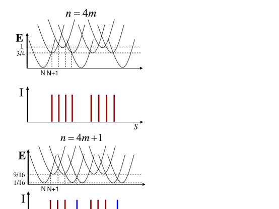
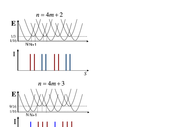
Figure 3: Schematic picture of the Coulomb blockade peaks for the $k=4$ RR state (we chose $s=0$ for convenience). The total energy of the dot, $E_{c}+E_{\psi}$, is plotted for every value of $n$ and $N_{e}$. The parabolic shape of the energy curve is due to the form of the charging energy, and the shift of the bottom of these parabolas is given by $E_{\psi}$. Coulomb blockade peaks appear when two neighboring parabolas intersect.

IV.1.2 Coulomb blockade in the presence of bulk-edge relaxation

If the area of the dot is varied slowly with respect to the relaxation rate, then each electron has time to relax onto the lowest energy state by changing the fusion channel of the edge quasiparticles and the bulk quasiholes.

Each electron entering the dot will occupy the first mode of $\psi_{k-1}$ operating on a highest weight state, $|\sigma_{\ell}\rangle$, which is dictated by the number of quasiholes in the bulk and the number of electrons $N_{e}$ that were inside the dot before the tunneling of the electron took place. Therefore the energy (in units of $2\pi v_{n}/L$) of the incoming electron is

$$h^{\ell}_{\ell-2}=h_{\ell}+\frac{\ell-1}{k}.$$ (31)

The above expression is simply the conformal dimension of the field which is the result of the fusion product of the incoming parafermion field, $\psi_{k-1}$, and the spin field $\sigma_{\ell}$ acting on the vacuum state (note that (31) is the correct expression for $\ell>1$, otherwise the restrictions in (12) should be taken into account). Now, by allowing the fusion channel of the bulk quasiholes to change, the energy of the edge state may be relaxed. Since the current $\mathbb{Z}_{k}$ charge of the edge is $\ell-2$, the fusion channel of the bulk quasihole is expected to change such that the energy of the edge is $h_{\ell-2}$ (this means that the fusion product of the fields on the edge changes to $\sigma_{\ell-2}$).

In order to calculate the spacings between Coulomb blockade peaks in this case, we use the form of equation (27), with a slight modification:

$$\Delta S=\frac{e}{n_{0}}+\frac{eL\nu}{2n_{0}\pi v_{c}} \left[E_{\psi}(N_{e}+2)-E_{\psi}(N_{e}+1)\right.$$ (32)

$$\left.-E^{\prime}_{\psi}(N_{e}+1)+E^{\prime}_{\psi}(N_{e})\right],$$

where $E_{\psi}(N_{e})$ is the energy of the edge state of a dot containing $N_{e}$ electrons before it had a chance to decay, and $E^{\prime}_{\psi}(N_{e})$ is the energy of the edge after the decay. For a particular value of $\ell>2$, these energies are given by

$$E_{\psi}(N_{e}+2)=\frac{2\pi v_{n}}{L}h^{\ell-2}_{\ell-4},\ E_{\psi}(N_{e}+1)=\frac{2\pi v_{n}}{L}h^{\ell}_{\ell-2},$$

$$E^{\prime}_{\psi}(N_{e}+1)=\frac{2\pi v_{n}}{L}h^{\ell-2}_{\ell-2},\ E^{\prime}_{\psi}(N_{e})=\frac{2\pi v_{n}}{L}h^{\ell}_{\ell},$$ (33)

therefore the area spacing between two peaks is given again by equation (28). However, if the initial charge of the edge was $\ell=1,2$, the spacing is given by equation (29).

The pattern of peaks we predict will be as follows. Bunching of peaks will still be observed for all the RR states with $k\geq 3$. However, the dependence of the pattern on the number of quasiholes in the bulk vanishes. The periodicity of this structure depends on $k$: if $k$ is even, the periodicity is $k/2$ and the pattern is of groups of $k/2$ peaks, while for odd $k$ the periodicity is $k$, and the pattern is of alternating groups of $(k-1)/2$ and $(k+1)/2$ peaks. foot (1)

For the case $k=2$, we find that when inelastic bulk-edge relaxation is allowed, the Coulomb blockade pattern will be the same as for Abelian fractional quantum Hall states, with a constant spacing between peaks. This means that for slow variation of the area of the dot, the even odd effect predicted in Ref. (Stern and Halperin, 2006) is smeared out. This smearing is a consequence of the parafermionic edge mode (which for $k=2$ is a Majorana fermion mode) staying unpopulated throughout the experiment. Whenever the addition of an electron into the dot attempts to populate this mode by a fermion, the bulk-edge relaxation mechanism makes the fermion tunnel inelastically into the bulk, where its presence does not involve any energy cost. It is important to stress, as we discuss in greater detail in the summary, that this smearing takes place only when the bulk-edge coupling induces inelastic relaxation, and the energy of the tunneling electron is dissipated away from the electronic system.

For other RR states, a change in the fusion channel of the bulk quasiholes, and as a result, also of the fields on the edge, can be understood in terms of tunneling of neutral particles as well. In this context, neutral means having no $\mathbb{Z}_{k}$ charge. The reason we allow for the bulk and the edge to exchange only particles with zero $\mathbb{Z}_{k}$ charge in order to relax the energy of the edge, is that fields that carry non trivial $\mathbb{Z}_{k}$ charge are always accompanied by a vertex operator that carries real electric charge. This physical assumption is required in order to keep the electron operator single-valued with respect to all possible excitation in the system. An electric charge is not allowed to tunnel freely into the bulk due to charging energy considerations.

Some more intuition on this relaxation process may be gained from Fig. 4, where we plot the energy as a function of the area. This graph, similarly to the graph presented in Fig. 3, shows a set of parabolas representing the energy of the dot as a function of its area. However, this time, different parabolas for the same value of $N_{e}$, corresponding to two different fusion channels of the parafermion fields on the edge, may participate in the process. Switching between two such parabolas is done by exchanging a neutral particle between the edge and the bulk. Note that only the crossing points marked by a black dot are those that indicate the location of a Coulomb peak. Other crossing points, such as the one denoted by $S_{1}$, correspond to higher order events we neglect, since both tunneling of an electron into the dot and relaxation take place simultaneously. Naturally, these processes are expected to occur on a longer time scale than relaxation alone, and are therefore at this point excluded from the discussion.

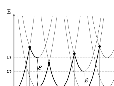
Figure 4: Schematic description of bulk - edge relaxation for the $k=3$ RR state. Every parabola on this graph represents the charging energy as a function of the area of the dot for a given number of electrons in the dot. The shift at the bottom of these parabolas is the part of the energy of the edge contributed by the parafermions. The initial state of the edge in this example is the vacuum state. Crossing points between neighboring parabolas that correspond to electron-tunneling events are marked by a black dot. The thick black curve represents the energy of the edge for any given value of the area. Note that two parabolas centered around the same point correspond to the same number of electrons in the dot, but a different fusion channel of the bulk quasiholes. A decay between two parabolas is an exchange of an $\varepsilon$ field between the edge and the bulk. We do not allow decay processes that require the tunneling and the decay to occur simultaneously, as in the region between the crossing points marked above $S_{1}$ and $S_{2}$.

V non-Abelian spin singlet states

The non-Abelian spin singlet states (NASS) at $\nu=\frac{2k}{2k+3}$ are close analogues of the clustered (parafermion) states of Read and Rezayi. The main difference is the role of the electron spin degree of freedom: while the RR states describe spin-polarized electrons, the spin-singlet states describe unpolarized electrons which make up a state that is a singlet under the spin $SU(2)$ symmetry. The quasiholes of smallest fractional charge ($q=\frac{1}{2k+3}$) are spin-1/2 particles. For $k>1$ they carry non-Abelian statistics. In the same way that the RR states generalize the $\nu=1/3$ Laughlin state, the $\nu=\frac{2k}{2k+3}$ spin-singlet states can be thought of as generalizations of the Abelian Halperin state at $\nu=2/5$.

Clustering of electrons in spin-singlet states is rather different and a bit more complicated than in the RR states. The RR state at $\nu=k/(k+2)$ can be thought of as a quantum fluid made of clusters of $k$ (spin polarized) electrons. The formation of such clusters is mirrored quite clearly in the relation $(\psi_{1})^{k}\sim\mathbf{1}$ satisfied by the fundamental parafermion $\psi_{1}$. The spin singlet states are associated with more complicated parafermion theories, formally denoted as $SU(3)_{k}/U(1)^{2}$. There are now two fundamental parafermions $\psi_{1}$ (associated to spin-up electrons) and $\psi_{2}$ (spin-down). The fusion rule $(\psi_{1}\psi_{2})^{k}\sim\mathbf{1}$ indicates that the smallest cluster with total spin zero is now composed of $2k$ electrons.

We will focus on the simplest example, which is the state with $k=2$ with filling fraction $\nu=4/7$. The $SU(3)_{2}/U(1)^{2}$ parafermion theory has central charge $c=6/5$. The $k=2$ state is made up of clusters of four electrons rather than two, each cluster having total spin zero. The CFT describing this state employs fields that are products of free boson vertex operators and parafermionic fields. There are now two fundamental bosons: $\varphi_{c}$ corresponding to charge and $\varphi_{s}$ giving the spin degrees of freedom. The parafermionic fields are again the source of the non-Abelian statistics of the quasiparticles.

For the $SU(3)_{2}/U(1)^{2}$ parafermionic theory, the parafermionic charge is a two component vector, and each field in the theory is labeled by two vectors, $\Phi^{\Lambda}_{\lambda}=\Phi^{(\Lambda_{1},\Lambda_{2})}_{(\lambda_{1},\lambda_{2})}$. The identification rules for the fields in this case areArdonne and Schoutens (2007)

$$\begin{array}[]{ll}\Phi^{(\Lambda_{1},\Lambda_{2})}_{(\lambda_{1},\lambda_{2})}\equiv\Phi^{(\Lambda_{1},\Lambda_{2})}_{(\lambda_{1}+4,\lambda_{2}-2)}\ ,&\Phi^{(\Lambda_{1},\Lambda_{2})}_{(\lambda_{1},\lambda_{2})}\equiv\Phi^{(\Lambda_{1},\Lambda_{2})}_{(\lambda_{1}-2,\lambda_{2}+4)}\ ,\\[5.69054pt] \Phi^{(\Lambda_{1},\Lambda_{2})}_{(\lambda_{1},\lambda_{2})}\equiv\Phi^{(2-\Lambda_{1}-\Lambda_{2},\Lambda_{2})}_{(\lambda_{1}+2,\lambda_{2})}\ ,&\Phi^{(\Lambda_{1},\Lambda_{2})}_{(\lambda_{1},\lambda_{2})}\equiv\Phi^{(\Lambda_{1},2-\Lambda_{1}-\Lambda_{2})}_{(\lambda_{1},\lambda_{2}+2)}\ .\\ \end{array}$$ (36)

Due to these identifications, the parafermion theory has eight fields, which we label in accordance with the notation of Ref. (Ardonne and Schoutens, 2007)

$$\begin{array}[]{cccc}\mathbf{1}=\Phi^{(0,0)}_{(0,0)},&\psi_{1}=\Phi^{(0,0)}_{(2,-1)},&\psi_{2}=\Phi^{(0,0)}_{(-1,2)},&\psi_{12}=\Phi^{(0,0)}_{(1,1)},\\ &\\ \sigma_{\downarrow}=\Phi^{(1,1)}_{(2,-1)},&\sigma_{\uparrow}=\Phi^{(1,1)}_{(-1,2)},&\sigma_{3}=\Phi^{(1,1)}_{(1,1)},&\rho=\Phi^{(1,1)}_{(0,0)}.\\ \end{array}$$ (40)

These fields obey the fusion rules presented in table 1. Their conformal dimensions are

$$h_{\psi}=\frac{1}{2},\quad h_{\sigma}=\frac{1}{10},\quad h_{\rho}=\frac{3}{5}.$$ (41)

We write $\vec{\varphi}=(\varphi_{c},\varphi_{s})$, where $\varphi_{c}$ and $\varphi_{s}$ are bosonic fields. Using the notation

$$\vec{\alpha}_{\uparrow}=\frac{1}{2}\left(\frac{1}{\sqrt{7}},1\right),\ \vec{\alpha}_{\downarrow}=\frac{1}{2}\left(\frac{1}{\sqrt{7}},-1\right),\ \vec{\alpha}_{3}=\left(\frac{1}{\sqrt{7}},0\right),$$

the three quasihole operators are

$$V_{qh}^{\uparrow}=\sigma_{\uparrow}e^{i\vec{\alpha}_{\uparrow}\cdot\vec{\varphi}},\quad V_{qh}^{\downarrow}=\sigma_{\downarrow}e^{i\vec{\alpha}_{\downarrow}\cdot\vec{\varphi}},\quad V_{qh}^{0}=\sigma_{3}e^{i\vec{\alpha}_{3}\cdot\vec{\varphi}},$$ (42)

corresponding to a spin-up quasihole with charge $1/7$, a spin-down quasihole with charge $1/7$, and a spin-less quasihole with charge $2/7$, respectively. The operators creating the two type of spinful electrons in the system are

$$V_{el}^{\uparrow}=\psi_{1}e^{i(\sqrt{7/4}\varphi_{c}+1/2\varphi_{s})}\ ,\quad V_{el}^{\downarrow}=\psi_{2}e^{i(\sqrt{7/4}\varphi_{c}-1/2\varphi_{s})},$$ (43)

Given this form of the electron operators, it is evident from the fusion rules that it takes four electrons to create a cluster with zero spin, since $\psi_{1}\times\psi_{2}\neq\mathbf{1}$.

$\times$		$\sigma_{\uparrow}$	$\sigma_{\downarrow}$	$\sigma_{3}$	$\rho$	$\psi_{1}$	$\psi_{2}$	$\psi_{12}\quad$
$\sigma_{\uparrow}$		$\mathbf{1}+\rho$
$\sigma_{\downarrow}$		$\psi_{12}+\sigma_{3}$	$\mathbf{1}+\rho$
$\sigma_{3}$		$\psi_{1}+\sigma_{\downarrow}$	$\psi_{2}+\sigma_{\uparrow}$	$\mathbf{1}+\rho$
$\rho$		$\psi_{2}$ + $\sigma_{\uparrow}$	$\psi_{1}+\sigma_{\downarrow}$	$\psi_{12}+\sigma_{3}$	$\mathbf{1}+\rho$
$\psi_{1}$		$\sigma_{3}$	$\rho$	$\sigma_{\uparrow}$	$\sigma_{\downarrow}$	$\mathbf{1}$
$\psi_{2}$		$\rho$	$\sigma_{3}$	$\sigma_{\downarrow}$	$\sigma_{\uparrow}$	$\psi_{12}$	$\mathbf{1}$
$\psi_{12}$		$\sigma_{\downarrow}$	$\sigma_{\uparrow}$	$\rho$	$\sigma_{3}$	$\psi_{2}$	$\psi_{1}$	$\mathbf{1}$

Table 1: Fusion rules of the parafermion and spin fields associated to the parafermion theory SU$(3)_{2}/[$U(1)$]^{2}$ .

V.1 Coulomb blockade regime

As we have mentioned above, the field theory describing the dynamical edge modes of the spin-singlet state at $\nu=4/7$ is a sum of three theories: two free chiral bosons, and a parafermionic field theory. The spectrum of the edge is therefore also made of three contributions

$$E=E_{c}+E_{s}+E_{\psi}$$ (44)

where $E_{c}$ labels the contribution of the charge boson $\varphi_{c}$, $E_{s}$ labels the contribution of the spin boson $\varphi_{s}$, and $E_{\psi}$ is the contribution from the parafermionic theory.

The contribution to the spectrum of the edge coming from the parafermions is again calculated by constructing the Hilbert space of parafermionic states, the set of highest weight states on which creation modes of the parafermions $\psi_{1}$ and $\psi_{2}$ operate.

The mode expansion of the parafermion $\psi_{\alpha}\equiv\Phi^{(0,0)}_{(\alpha_{1},\alpha_{2})}$ is given by

$$\psi_{\alpha}=\sum_{m}z^{-m-\frac{1}{2}}\psi^{(\alpha)}_{m},$$ (45)

where the mode indices $m$ may be integer or half-integer, depending on boundary conditions of the parafermion set by the field on which these parafermions act. For example, when acting on the vacuum state, $m\in\mathbb{Z}+1/2$, since the parafermion should obey periodic boundary conditions. When acting on any other field, $\Phi^{\Lambda}_{\lambda}$, the boundary conditions can easily be determined using the Operator Product Expansion between the two fields.

The charging energy as a function of the number of electrons in the dot may be found using the same considerations that were explained in Sec. II. It is given by Eq. (3). The energy cost associated with creating non-zero spin inside the dot will, by analogy, have the form

$$E_{s}=\frac{v_{s}}{4\pi}\int\left(\partial_{x}\varphi_{s}\right)^{2}dx=\frac{\pi v_{s}}{4L}N_{s}^{2}$$ (46)

with $N_{s}$ being the net number of unpaired spins on the edge.

We assume that the region outside the dot, the leads from which electrons tunnel into and out of the dot, contains electrons of both spins, and that both spins are equally available, such that finding the lowest energy state of $j$ parafermions on the edge is not constrained by availability of a certain type of spin. Since the ground state of the dot is a spin singlet, breaking ”spin neutrality” must cost a certain amount of energy, and this energy cost given by Eq. (46) will influence the order in which electrons enter the dot.

Using the same argument we used in section IV.1, we now turn to construct the lowest lying energy states of the parafermion theory. This time, however, we must take into account the spin of the incoming electron in order to determine the order in which the parafermion modes are applied to the highest weight state. While the charging energy is unavoidable, the other two components of the energy may compete with each other. We now turn to evaluate a particular example in order to demonstrate the effect of this competition.

We start from the case when the bulk of the dot does not include any quasiholes ($n=0$). The fusion rules and the requirement that the ground state of the dot is a spin singlet imply that the electrons cluster into groups of $4$. If the total number of electrons in the dot is not divisible by $4$, the remainder accumulate at the edge, occupying charge, spin and parafermionic modes. The parafermionic state of the edge is then obtained by applying $j$ parafermion operators to the vacuum, with $0\leq j\leq 3$. For simplicity, we start from a situation where the initial number of spin-up electrons, $N^{0}_{\uparrow}$, is equal to the number of spin down electron, $N^{0}_{\downarrow}$, which is even. Therefore the highest weight state of the edge theory is $|0\rangle$, the vacuum state, and the initial number of occupied edge modes is zero.

The first electron to tunnel into the dot will create non-zero total spin inside it. Since the energy cost involved, $E_{s}=\pi v_{s}/4L$, cannot be avoided and is the same for both types of spin we choose without loss of generality that this electron is a spin up electron. The modes $m$ of the parafermion part of the electron operator, $\psi_{1}$, will be half-integer, and therefore the state with one occupied parafermion mode is

$$\psi^{(1)}_{-\frac{1}{2}}|0\rangle$$ (47)

and the corresponding energy is $E_{\psi}=1/2(2\pi v_{n}/L)$.

We now estimate the energy cost for the tunneling of the second electron assuming that the first one was a spin up electron ($\psi_{1}$). If the second electron is a spin up electron, we will again need to pay energy for increasing the total spin of the system. The boundary conditions on the $\psi_{1}$ field are periodic, and therefore the parafermionic edge state will be

$$\psi^{(1)}_{1/2}\psi^{(1)}_{-1/2}|0\rangle,$$ (48)

with $E_{\psi}=0$ and $E_{s}=4(\pi v_{s}/4L)$.

On the other hand, if the second electron is a spin down electron, the spin of the system will be reduced back to zero. This way, the energetic cost associated with spin polarization is avoided. The boundary conditions on the $\psi_{2}$ field are antiperiodic, since $\psi_{1}\cdot\psi_{2}\sim z^{-1/2}\psi_{12}$, and therefore the state will be

$$\psi^{(2)}_{0}\psi^{(1)}_{-1/2}|0\rangle,$$ (49)

with $E_{\psi}=1/2(2\pi v_{n}/L)$, and the energy due to spin is $E_{s}=0$.

Comparing the two scenarios in which two electrons tunneled into the edge of the system, we find that in order to determine which state has lower energy we must consider the ratio between $v_{n}$ and $v_{s}$. Bringing in a spin down electron as the second electron is an energetically favorable process as long as $v_{n}/v_{s}<1$, while when $v_{n}/v_{s}>1$, the lowest energy will correspond to a state of two electrons with the same spin.

If $v_{n}/v_{s}<1$, then the state of three electrons on the edge must correspond to

$$\psi^{(1)}_{0}\psi^{(2)}_{0}\psi^{(1)}_{-1/2}|0\rangle,$$ (50)

with $E_{\psi}=1/2(2\pi v_{n}/L)$ and $E_{s}=(\pi v_{s}/4L)$. Finally, the fourth electron entering the dot will have spin down, setting the total spin of the dot back to zero. The parafermion state of four parafermions is identified with the vacuum state.

Since the lowest energy of a state with $j$ parafermions is always given by the conformal dimension of the field which is the result of the fusion product of all the parafermions, the tunneling sequences can intuitively be described using a simple diagram. The sequence corresponding with the case $v_{n}/v_{s}>1$, can be represented diagrammatically as

$$\mathbf{1}\stackrel{{\scriptstyle\psi_{1}}}{{\longrightarrow}}\psi_{1}\stackrel{{\scriptstyle\psi_{1}}}{{\longrightarrow}}\mathbf{1}\stackrel{{\scriptstyle\psi_{2}}}{{\longrightarrow}}\psi_{2}\stackrel{{\scriptstyle\psi_{2}}}{{\longrightarrow}}\mathbf{1}$$ (51)

The parafermion above the arrow in the diagram is the parafermion added to the edge state, and the fields at the tip of an arrow is the result of the fusion product of the field at the beginning of the arrow with that parafermion. The energies are given by

$$E_{0}=E_{c}(N_{e})$$

$$E_{1}=E_{c}(N_{e}+1)+\frac{\pi v_{n}}{L}+\frac{\pi v_{s}}{4L}$$

$$E_{2}=E_{c}(N_{e}+2)+\frac{\pi v_{s}}{L}$$

$$E_{3}=E_{c}(N_{e}+3)+\frac{\pi v_{n}}{L}+\frac{\pi v_{s}}{4L}$$ (52)

The sequences corresponding to the case $v_{n}/v_{s}<1$ are either

$$\mathbf{1}\stackrel{{\scriptstyle\psi_{1}}}{{\longrightarrow}}\psi_{1}\stackrel{{\scriptstyle\psi_{2}}}{{\longrightarrow}}\psi_{12}\stackrel{{\scriptstyle\psi_{1}}}{{\longrightarrow}}\psi_{2}\stackrel{{\scriptstyle\psi_{2}}}{{\longrightarrow}}\mathbf{1},$$ (53)

or alternatively

$$\mathbf{1}\stackrel{{\scriptstyle\psi_{1}}}{{\longrightarrow}}\psi_{1}\stackrel{{\scriptstyle\psi_{2}}}{{\longrightarrow}}\psi_{12}\stackrel{{\scriptstyle\psi_{2}}}{{\longrightarrow}}\psi_{1}\stackrel{{\scriptstyle\psi_{1}}}{{\longrightarrow}}\mathbf{1}$$ (54)

And this time the energies are given by

$$E_{0}=E_{c}(N_{e})$$

$$E_{1}=E_{c}(N_{e}+1)+\frac{\pi v_{n}}{L}+\frac{\pi v_{s}}{4L}$$

$$E_{2}=E_{c}(N_{e}+2)+\frac{\pi v_{n}}{L}$$

$$E_{3}=E_{c}(N_{e}+3)+\frac{\pi v_{n}}{L}+\frac{\pi v_{s}}{4L}$$ (55)

Of course, interchanging $\psi_{1}$ with $\psi_{2}$ in these diagrams leaves the energies at each stage completely invariant.

Using Eq. (3) and $(\ref{coulomb-peaks})$, we may find the area, which appears in the expression for the charging energy, for which transport through the dot is allowed. Then we may calculate the area spacing between peaks. We find that the two sequences above correspond to two different Coulomb peak structures. The first sequence corresponds to

$$\Delta S_{1}=\frac{e}{n_{0}}\left(1+\nu\frac{v_{s}}{4v_{c}}-\nu\frac{v_{n}}{v_{c}}\right)$$

$$\Delta S_{2}=\frac{e}{n_{0}}\left(1-3\nu\frac{v_{s}}{4v_{c}}+\nu\frac{v_{n}}{v_{c}}\right)$$

$$\Delta S_{3}=\frac{e}{n_{0}}\left(1+\nu\frac{v_{s}}{4v_{c}}-\nu\frac{v_{n}}{v_{c}}\right)$$

$$\Delta S_{4}=\frac{e}{n_{0}}\left(1+\nu\frac{v_{s}}{4v_{c}}+\nu\frac{v_{n}}{v_{c}}\right)$$ (56)

while the second sequence corresponds to

$$\Delta S_{1}=\frac{e}{n_{0}}\left(1-\nu\frac{v_{s}}{4v_{c}}-\frac{1}{2}\nu\frac{v_{n}}{v_{c}}\right)$$

$$\Delta S_{2}=\frac{e}{n_{0}}\left(1+\nu\frac{v_{s}}{4v_{c}}\right)$$

$$\Delta S_{3}=\frac{e}{n_{0}}\left(1-\nu\frac{v_{s}}{4v_{c}}-\frac{1}{2}\nu\frac{v_{n}}{v_{c}}\right)$$

$$\Delta S_{4}=\frac{e}{n_{0}}\left(1+\nu\frac{v_{s}}{4v_{c}}+\nu\frac{v_{n}}{v_{c}}\right)$$ (57)

These spacings repeat themselves as the area is varied. It is obvious that they fluctuate around the value anticipated to occur for the Abelian states, just as in the case of the RR series.

It is instructive to compare the $k=2$ spin-singlet state to the $k=2$ RR state (a.k.a. the Moore-Read state). While both states can be obtained as maximal density zero-energy eigenstate of the same ‘pairing’ Hamiltonian Ardonne et al. (2001), the periodicity in the Coulomb blockade peak structure is different. For the Moore-Read the maximal periodicity is 2 while for the spin singlet state we find a periodicity of 4, in agreement with the physical picture where the state is built up from clusters having 4 electrons each.

When $n$ is non-zero, the requirement for spin-neutrality leads to $N_{\uparrow}+n_{\uparrow}=N_{\downarrow}+n_{\downarrow}$, where $n_{\uparrow(\downarrow)}$ denotes the number of spin-up (down) quasiholes and $N_{\uparrow(\downarrow)}$ denotes the number of spin-up (down) electrons . By the same considerations applied for the RR states, the fusion channel of the bulk quasiholes directly influences the fusion channel of the spin fields on the edge, thus determining the highest weight state on which the modes of the parafermions act. Also, these fusion channels at the beginning of the experiment are fixed such that the edge has the lowest possible energy.

Looking at the fusion rules (Table 1), we find that the fusion channel of the bulk quasiholes will be the same as the fusion channel of the spin fields on the edge. Having an initial number of spin up electrons on the edge, given by $[N_{\uparrow}]_{2}$, or spin down electrons, given by $[N_{\downarrow}]_{2}$, will influence both fusion channels.

Let us consider an example for concreteness. Suppose that the possible fusion channels of quasiholes in the bulk are $\psi_{2}+\sigma_{\uparrow}$. If $[N_{\uparrow}]_{2}=[N_{\downarrow}]_{2}=0$, the requirement that the edge has the lowest possible energy fixes the fusion channel of the edge to be $\sigma_{\uparrow}$, since it has a lower conformal dimension. However, if this is not the case, the fusion channel of the bulk quasiholes may be $\psi_{2}$, such that the edge is in the vacuum state. This may occur when $[N_{\uparrow}]_{2}=0$ but $[N_{\downarrow}]_{2}=1$.

In general, there are four possible highest weight states on the edge: $|0\rangle,|\sigma_{\uparrow}\rangle,|\sigma_{\downarrow}\rangle$ and $|\sigma_{3}\rangle$, and it is difficult to predict how they correspond to the exact number of quasiholes in the dot, and to the initial number of electrons on the edge, as we have done for the RR states. This is true mostly because there may also be quasiholes of zero spin in the bulk which do not contribute to the total spin, but may change the possible fusion channel of the bulk (and therefore the one of the edge). Consequently, we study tunneling of electrons into an edge characterized by each of these highest weight states, knowing that initially, the total spin of the dot was zero, and by applying the same logic we applied for the vacuum state above. The results are summarized in Table 2.

If the system is allowed to to relax into its ground state after each tunneling event of an electron into the dot, i.e, the fusion channel of the bulk quasiholes is allowed to change when the new electron is added, the sequences appearing in Table 2 will change whenever one of the fields in the chain is not a primary field. Noting that, we realize that the sequences that may change are the ones starting with the identity field, and the second sequence constructed from the primary field $|\sigma_{3}\rangle$, appearing last on Table 2. When drawing the new sequences we will denote a decay to a lower energy state (switching to a field with the same charge, but with lower conformal dimension) by a dashed arrow.

Let us see how this generalization applies to the sequences that formally started with the identity operator. We therefore start with the case where the fusion channel of the bulk quasiholes is such that the initial state of the edge is either $1$ or $\rho$, and may switch between these two in order to minimize the energy. This switching is again done via the exchange of a neutral particle, as we discussed at the end of Sec. IV.1. In this case, the neutral particle is $\rho$. Before any electron-tunneling occurs, the state of the edge will be the vacuum state, and therefore our sequence begins with the identity field again. It will be, for example

$$\mathbf{1}\stackrel{{\scriptstyle\psi_{1}}}{{\longrightarrow}}\psi_{1}\dashrightarrow\sigma_{\downarrow}\stackrel{{\scriptstyle\psi_{2}}}{{\longrightarrow}}\sigma_{3}\stackrel{{\scriptstyle\psi_{1}}}{{\longrightarrow}}\sigma_{\uparrow}\stackrel{{\scriptstyle\psi_{2}}}{{\longrightarrow}}\rho\dashrightarrow\mathbf{1}$$ (58)

for the limit in which the spin energy is the dominant energy ($v_{n}/v_{s}<1$). The energy cost for each of the tunneling electrons and the energy of the edge after relaxation takes place are again easily calculated using the conformal dimension of the parafermionic fields as well as Eqs. (3) and (46). Other ordering of $\psi_{1}$ and $\psi_{2}$ that minimize the spin energy will yield the same set of energies. Plugging these into equation (32), we then find that the set of spacings between peaks changes from the one appearing in Eq. (V.1) to the following set

$$\Delta S_{1}=\frac{e}{n_{0}}\left(1+\nu\frac{v_{s}}{4v_{c}}\right)$$ (59)

$$\Delta S_{2}=\frac{e}{n_{0}}\left(1-\nu\frac{v_{s}}{4v_{c}}+\frac{1}{2}\nu\frac{v_{n}}{v_{c}}\right)$$

$$\Delta S_{3}=\frac{e}{n_{0}}\left(1+\nu\frac{v_{s}}{4v_{c}}\right)$$

$$\Delta S_{4}=\frac{e}{n_{0}}\left(1-\nu\frac{v_{s}}{4v_{c}}-\frac{1}{2}\nu\frac{v_{n}}{v_{c}}\right)$$

which is slightly different but again corresponds to a periodicity of $4$ for the Coulomb Blockade structure.

In the opposite limit where the energy associated with the spin excitation is smaller, the sequence of fields will be

$$\mathbf{1}\stackrel{{\scriptstyle\psi_{1}}}{{\longrightarrow}}\psi_{1}\dashrightarrow \sigma_{\downarrow}\stackrel{{\scriptstyle\psi_{2}}}{{\longrightarrow}}\sigma_{3}\stackrel{{\scriptstyle\psi_{1}}}{{\longrightarrow}}$$

$$\sigma_{\uparrow}\stackrel{{\scriptstyle\psi_{1}}}{{\longrightarrow}}\sigma_{3}\stackrel{{\scriptstyle\psi_{2}}}{{\longrightarrow}}\sigma_{\downarrow}\stackrel{{\scriptstyle\psi_{2}}}{{\longrightarrow}}\sigma_{3}\stackrel{{\scriptstyle\psi_{1}}}{{\longrightarrow}}\sigma_{\uparrow}\stackrel{{\scriptstyle\psi_{1}}}{{\longrightarrow}}\sigma_{3}....$$

and so on. The above sequence shows that after the first electron tunnels into the dot, the sequence turns out to be the same as if the highest weight state of the dot was $|\sigma_{3}\rangle$, and therefore the spacings will be the same as for that case (see Table 2).

When the fusion channel of the bulk quasiholes is such that the initial state of the edge is $\sigma_{3}$, and the spin energy is the dominant one, the sequence of fields generalizes to

$$\sigma_{3}\stackrel{{\scriptstyle\psi_{1}}}{{\longrightarrow}}\sigma_{\uparrow}\stackrel{{\scriptstyle\psi_{2}}}{{\longrightarrow}}\rho\dashrightarrow\mathbf{1}\stackrel{{\scriptstyle\psi_{1}}}{{\longrightarrow}}\psi_{1}\dashrightarrow\sigma_{\downarrow}\stackrel{{\scriptstyle\psi_{2}}}{{\longrightarrow}}\sigma_{3}.$$ (61)

Note that this sequence is identical to sequence (58), and following from it is the same set of spacings given in Eq. (59).

In conclusion, we have found that depending on the highest weight state of the edge, the periodicity of the Coulomb blockade peak pattern will be either $4$ or $2$. Also, in contrast with the result we obtained for the $k=2$ RR state, where the time scale on which the area is varied strongly influenced the periodicity, we find that for the state at $\nu=4/7$, while the spacings themselves are affected by the relaxation of the edge, the periodicity of the peak pattern remains unaffected.

V.2 Lowest order interference

In this section we find the interference term of Eq. (1) when the bulk is at the $\nu=4/7$ NASS state. We use the CFT input detailed at the beginning of Sec. V.

Lowest order interference for the RR series of states was studied before in Ref. (Bonderson et al., 2006b), and a general expression for the interference term was obtained. The approach of Ref. (Bonderson et al., 2006b) relied on studying the properties of the modular S-matrix relevant for the parafermion and free chiral boson CFTs.

For convenience, in this section we shall refer to parafermionic fields with a fusion product that may yield more than one possible outcome as ”non-Abelian” fields (those are the three $\sigma$’s and $\rho$), and to those who always fuse to one field as ”Abelian” (the three $\psi$’s and $\mathbf{1}$). As we will see, there will be a crucial difference between the interference term in the case where the fusion product of the bulk quasiholes results in a non-Abelian or an Abelian filed. This is also true for the RR states, as was demonstrated before in Refs. (Stern and Halperin, 2006; Bonderson et al., 2006a, b; Chung and Stone, 2006).

Every one of the $n$ localized bulk quasiholes, and also the quasiholes propagating along the edge are either spin-up, spin-down, or spin-less, corresponding to the operators listed in Eq. (42). Again, we denote by $n_{\uparrow}$ the number of localized quasiholes with spin up and by $n_{\downarrow}$ the number of localized quasiholes with spin down. The number of localized spin-less quasiholes is denoted $n_{3}$, such that $n=n_{\uparrow}+n_{\downarrow}+n_{3}$.

The result of the fusion product of all the quasiholes localized in the bulk into a single field can be obtained by fusing all the bosonic contributions into the single bosonic operator, $e^{i\frac{1}{2}\left(\frac{n_{\uparrow}+n_{\downarrow}+2n_{3}}{\sqrt{7}},n_{\uparrow}-n_{\downarrow}\right)\cdot\vec{\varphi}}$, and fusing all the spin fields of the quasihole operators into a single parafermionic field. The operator that is obtained represents the internal state of the island between the two point contacts, and will ultimately determine the form of the interference term we wish to calculate.

We assume here that the bulk quasiholes have a definite fusion channel. Although in principle the fusion product of all the spin fields has two possible outcomes, it was shown in a previous work Bonderson et al. (2008) that the measurement procedure collapses this superposition onto a particular fusion channel. We do not elaborate on the collapse process here, but rather refer the interested reader to Ref. (Bonderson et al., 2008) for more details.

The fusion product of $n$ spin fields of different types may have eight different results, due to the existence of eight parafermionic fields of the $SU(3)_{2}/U(1)^{2}$ coset. Accordingly, the state of the island may be represented by eight different operators. For a fixed value of $n_{\uparrow}$, $n_{\downarrow}$ and $n_{3}$, the state of the island will be one of two fields, Abelian or non-Abelian according to the fusion rules (Table 1).

We now study the interference between the two partial waves $|\psi_{L}\rangle$ and $|\psi_{R}\rangle$ discussed in Sec. II, and examine how different internal states of the dot affect them, hence influencing the interference term of the backscattered current.

When the internal state of the island is represented by a non-Abelian field, the fusion product of this field with an incoming quasihole on the edge is a superposition of two fields. To each of these we assign a state. We denote the two states by $|0\rangle$ and $|1\rangle$, referring to an Abelian and non-Abelian field correspondingly. For example, if there is only one localized spin up quasihole in the bulk, and the edge quasihole also has spin up, the two spin fields of the type $\sigma_{\uparrow}$ fuse as follows: $\sigma_{\uparrow}\sigma_{\uparrow}\sim 1+\rho$. Therefore, we say that the system is in a superposition state $|\psi\rangle=a_{0}|0\rangle+a_{1}|1\rangle$, with $|a_{0}|^{2}+|a_{1}|^{2}=1$. The state $|0\rangle$ corresponds to the Abelian field $\mathbf{1}$, and the state $|1\rangle$ corresponds to the non-Abelian field $\rho$. Note that the two partial waves $|\psi_{L,R}\rangle$ describe the state of the $n$ localized quasiholes and the incoming edge quasihole.

The two partial waves can be written, using the above notation, as follows

$$|\psi_{L}\rangle=a_{0}|0\rangle+a_{1}|1\rangle$$ (62)

$$|\psi_{R}\rangle=(e^{i\phi_{R}}a_{0}|0\rangle+a_{1}|1\rangle)e^{i\beta+i\phi_{\Delta}+i\phi_{B}}$$ (63)

The phase $\phi_{B}$ is contributed by the bosonic exponents carrying the charge and the spin of the quasiholes. The origin of the phases $\phi_{\Delta}$, and $\phi_{R}$ lies in the conformal nature of the parafermionic fields, and we explain how to determine them below.

In case the parafermionic operator of the island is Abelian, the coefficient $a_{0}$ is zero, and $|\psi_{R}\rangle=|1\rangle e^{i\beta+i\phi_{\Delta}^{A}+i\phi_{B}}$ (the superscript $A$ is added to $\phi_{\Delta}$ to indicate that the internal state of the dot corresponds to an Abelian field). In the case where $a_{0}=0$, the interference term contributed to the backscattered current by the two partial waves, proportional to the real part of the overlap $\langle\psi_{L}|\psi_{R}\rangle$, is given by

$$\cos{({\rm\arg}\langle\psi_{L}|\psi_{R}\rangle_{A}})=\cos{(\beta+\phi_{\Delta}^{A}+\phi_{B})}$$ (64)

When the parafermionic operator of the island is non-Abelian, the overlap is given by

$$\langle\psi_{L}|\psi_{R}\rangle_{NA}=(e^{i\phi_{R}}|a_{0}|^{2}+|a_{1}|^{2})e^{i\beta+i\phi_{\Delta}^{NA}+i\phi_{B}}.$$ (65)

The ratio between the overlap in equation (64) and the overlap in the case where the parafermionic operator of the island is non-Abelian is given by

$$\frac{\langle\psi_{L}|\psi_{R}\rangle_{NA}}{\langle\psi_{L}|\psi_{R}\rangle_{A}}=(e^{i\phi_{R}}|a_{0}|^{2}+|a_{1}|^{2})e^{i(\phi_{\Delta}^{NA}-\phi_{\Delta}^{A})}.$$ (66)

and will determine both the relative amplitude and the phase shift between the two cases.

• Determining the phases $\phi_{\Delta}^{A},\phi_{\Delta}^{NA},\phi_{R}$, and $\phi_{B}$.

  As was mentioned before, the fusion of $n$ quasiholes results in a parafermion multiplied by a bosonic vertex operator of the form

  $$e^{i\left(n_{\uparrow}\vec{\alpha}_{\uparrow}+n_{\downarrow}\vec{\alpha}_{\downarrow}+n_{3}\vec{\alpha}_{3}\right)\cdot\vec{\varphi}}=e^{i\frac{1}{2}\left(\frac{n_{\uparrow}+n_{\downarrow}+2n_{3}}{\sqrt{7}},n_{\uparrow}-n_{\downarrow}\right)\cdot\vec{\varphi}}.$$ (67)

  An incoming quasihole carries, in general, a bosonic factor of the form $e^{i\vec{\alpha}_{ex}\cdot\vec{\varphi}}$, with $\vec{\alpha}_{ex}=(\alpha_{c},\alpha_{s})$ being $\alpha_{\uparrow}$, $\alpha_{\downarrow}$ or $\alpha_{3}$. The OPE of the two vertex operators is

  $$e^{i\vec{\alpha}_{ex}\cdot\vec{\varphi}}(z)e^{i\frac{1}{2}\left(\frac{n_{\uparrow}+n_{\downarrow}+2n_{3}}{\sqrt{7}},n_{\uparrow}-n_{\downarrow}\right)\cdot\vec{\varphi}}(0)\ \sim$$

  $$z^{f(n_{\uparrow},n_{\downarrow},n_{3})}\,e^{i\frac{1}{2}\left(\frac{n_{\uparrow}+n_{\downarrow}+2n_{3}}{\sqrt{7}}+2\alpha_{c},n_{\uparrow}-n_{\downarrow}+2\alpha_{s}\right)\cdot\vec{\varphi}}(0),$$

  where

  $$f(n_{\uparrow},n_{\downarrow},n_{3})=\frac{1}{2}\left[\frac{(n_{\uparrow}+n_{\downarrow}+2n_{3})\alpha_{c}}{\sqrt{7}}+(n_{\uparrow}-n_{\downarrow})\alpha_{s}\right].$$

  Therefore,

  $$\phi_{B}=\pi\left[\frac{(n_{\uparrow}+n_{\downarrow}+2n_{3})\alpha_{c}}{\sqrt{7}}+(n_{\uparrow}-n_{\downarrow})\alpha_{s}\right].$$ (69)

  The phases $\phi_{\Delta}^{NA},\phi_{\Delta}^{A}$ and $\phi_{R}$ all depend on the conformal dimension of the parafermionic fields. We now demonstrate how to calculate them for a particular example (we leave out the bosonic part of the quasihole operators). Suppose that the fusion of $n$ quasiholes on the island can result in one of the following two parafermions: $\psi_{2}$ or $\sigma_{\uparrow}$. Suppose that the incoming edge quasihole has spin up. If the quasiholes on the dot fused to the Abelian field $\psi_{2}$, the OPE of the island’s operator with the incoming quasiholes is

  $$\psi_{2}\cdot\sigma_{\uparrow}\sim z^{h_{\rho}-h_{\sigma}-h_{\psi}}\rho.$$ (70)

  Therefore, the phase accumulated when the quasihole encircles the island is $\phi_{\Delta}^{A}=2\pi(h_{\rho}-h_{\sigma}-h_{\psi})=0$.

  If the $n$ quasiholes in the dot fused to yield the non-Abelian field $\sigma_{\uparrow}$, the OPE of the island’s operator with the incoming quasiholes is

  $$\sigma_{\uparrow}\sigma_{\uparrow}\sim z^{-2h_{\sigma}}\mathbf{1}+z^{h_{\rho}-2h_{\sigma}}\rho=(z^{-h_{\rho}}\mathbf{1}+\rho)z^{h_{\rho}-2h_{\sigma}}.$$ (71)

  From the above equation we conclude that $\phi_{R}=-2\pi h_{\rho}=-6\pi/5$, and $\phi_{\Delta}^{NA}=2\pi(h_{\rho}-2h_{\sigma})=4\pi/5$.

• Determining the values of $|a_{0}|^{2}$ and $|a_{1}|^{2}$

  The coefficients $|a_{0}|^{2},|a_{1}|^{2}$ are the probabilities that the quasihole encircling the island fuses with the localized bulk quasiholes into Abelian and non-Abelian fields, respectively.

  In the general context of models for non-Abelian anyons Bonderson et al. (2008); Preskill (2004), the probability that two uncorrelated anyons, $a$ and $b$, fuse into a third anyon $c$ is given by (see Ref. (Preskill, 2004))

  $$P(ab\rightarrow c)=N_{ab}^{c}\frac{d_{c}}{d_{a}d_{b}}$$ (72)

  where $d_{a},d_{b}$ and $d_{c}$ are the quantum dimensions of the anyons. The coefficient $N_{ab}^{c}$ is in general a non-negative integer determined by the fusion rules, and indicates the number of different way the anyons $a$ and $b$ can be combined to form $c$. In our case it is either zero or one, depending on whether the fusion rules allow $a$ and $b$ to fuse to $c$.

  The quantum dimension is a parameter that controls the rate in which the Hilbert space of a system of $n$ anyons of a certain type grows. For a large number of such anyons, the number of states scales as $d^{n}$. For Abelian particles $d=1$, while non-Abelian particles have $d>1$.

  The expression for the overlap between the two partial waves $|\psi_{L,R}\rangle$ can therefore be written as follows

  $$\langle\psi_{L}|\psi_{R}\rangle_{NA}=\frac{1}{d_{bulk}d_{qh}}(e^{i\phi_{R}}+d_{1})e^{i\beta+i\phi_{\Delta}^{NA}+i\phi_{B}}.$$ (73)

  Where $d_{bulk}$ and $d_{qh}$ are the quantum dimensions of the bulk and of the edge quasihole respectively. The quantum dimension $d_{1}$ is that of the non-Abelian field that is the result of the fusion product of both. Note that this expression is exactly the expression for the monodromy matrix element calculated in Ref. (Bonderson et al., 2008)

  $$M_{ab}=\frac{1}{d_{a}d_{b}}\sum_{c}N_{ab}^{c}d_{c}e^{2\pi i(s_{c}-s_{a}-s_{b})}$$ (74)

  where $s_{i}$ is the scaling dimension of the relevant anyon. In our case, $a$ represents the edge qusihole and $b$ represents the composite made of a group of qusiholes in the bulk.

  Taking for example the neutral part of the spin-up quasihole $\sigma_{\uparrow}$, we use the fusion rules to count how many states there are for $n$ such quasiholes:

  $$\sigma_{\uparrow}\sigma_{\uparrow}=\mathbf{1}+\rho$$

  $$\sigma_{\uparrow}\sigma_{\uparrow}\sigma_{\uparrow}=\psi_{2}+2\sigma_{\uparrow}$$

  $$\sigma_{\uparrow}\sigma_{\uparrow}\sigma_{\uparrow}=2\mathbf{1}+3\rho$$

  $$\sigma_{\uparrow}\sigma_{\uparrow}\sigma_{\uparrow}\sigma_{\uparrow}=3\psi_{2}+5\sigma_{\uparrow}...$$

  The number of states for $n$ quasiholes is a Fibonacci number. For a large value of $n$, this number scales as $\tau^{n}$, where $\tau$ is the Golden Ratio.

  Following the same considerations one finds that for the $SU(3)_{2}$ parafermionic fields, there are two values for the quantum dimension: The quantum dimension of the Abelian fields $\mathbf{1},\psi_{i}$ is $d=1$, while that of the non-Abelian fields $\rho,\sigma_{i}$ is $d=\tau$. Therefore

  $$|a_{1}|^{2}=\frac{1}{\tau},\quad|a_{0}|^{2}=\frac{1}{\tau^{2}}.$$ (75)

Plugging the values of $\phi_{R}$, $\phi_{\Delta}^{NA}$ and $\phi_{\Delta}^{A}$ from the above example into Eq. (66), along with the coefficients Eq. (75), and using the fact that $\tau=2\cos(\pi/5)$, we find

$$\frac{\langle\psi_{L}|\psi_{R}\rangle_{NA}}{\langle\psi_{L}|\psi_{R}\rangle_{A}}=-\tau^{-2}.$$ (76)

From Eq. (76) we conclude that the interference term is suppressed by a factor of $\tau^{-2}$ when the parafermionic operator of the island is non-Abelian.

It is straightforward to calculate the ratio Eq. (66) for all other possible operators of the island. The result always turns out the same and given by Eq. (76). The interference term is therefore

$$(-\tau^{-2})^{N_{\phi}}$$

$$\times\cos\left(\beta+\pi\frac{(n_{\uparrow}+n_{\downarrow}+2n_{3})\alpha_{c}}{\sqrt{7}}+\pi(n_{\uparrow}-n_{\downarrow})\alpha_{s}+\phi_{\Delta}^{A}\right)$$

$$=(-\tau^{-2})^{N_{\phi}}\cos\left(\beta+8\pi\frac{(n_{\uparrow}+n_{\downarrow}+2n_{3})\alpha_{c}}{\sqrt{7}}\right).$$ (77)

Here $\phi_{\Delta}^{A}=\pi(\lambda_{1}^{bulk}\lambda_{2}^{qh}+\lambda_{2}^{{bulk}}\lambda_{1}^{qh})$ is $0$ or $\pi$ (up to $2\pi$) depending on the specific Abelian field that may result from fusing $n$ bulk quasiholes. The vector $(\lambda_{1},\lambda_{2})$ is given for each operator in equation (40), $\lambda_{i}^{bulk}$ are the components of the vector that corresponds to the fusion product of the bulk quasiholes, and $\lambda_{i}^{qh}$ are the components of the vector that corresponds to the quasihole that tunnels across the point-contact. The second line of the equation is obtained from the first with some algebra. The number $N_{\phi}$ is either $0$ or $1$ depending on whether the fusion product of the quasiholes on the dot was an Abelian or non-Abelian field. Eq. (77) shows that the damping factor that multiplies the interference term is the same as the one predicted to appear for the $k=3$ RR state. This is a manifestation of the so-called ”level-rank duality” between $SU(3)_{2}$ and $SU(2)_{3}$, see Ref. (Ardonne et al., 2001). This result agrees with the one calculated using the modular S-matrixArdonne in a similar fashion to the calculation presented in Ref. (Bonderson et al., 2006b) for lowest order interference in the RR series.

The above result is calculated without making any assumptions on the nature of the edge qusiholes that tunnels across the point contact, and is therefore general. However, it is expected that the most prominent contribution to these tunneling events will come from the quasihole with the lowest conformal dimension. For that reason, one may expect mostly spinless quasiholes to tunnel across the junction. The interference term for these quasiparticle is given by equation (77) with $\alpha_{c}=1/\sqrt{7}$ and $\alpha_{s}=0$.

VI Summary

In this work we studied transport through a device known as the two point-contact (or the Fabry-Perot) interferometer formed using edge states of non-Abelian quantum Hall phases. We have focused on the RR series at filling factor $\nu=2+\frac{k}{k+2}$, and on one of the spin singlet states that may be appropriate to describe the plateau at filling factor $4/7$.

For the limit of strong quasihole backscattering at the two point contacts, where the topmost partially filled level forms a closed trajectory around the ”island” formed between the point contacts, transport is characterized by a series of Coulomb blockade peaks in the conductance as a function of the area enclosed by this trajectory.

For the RR states we explained in details the results obtained in Ref. (Ilan et al., 2008), and analyzed the effect of relaxation of the edge states of the parafermionic theory into states with lower energy by adjusting the fusion channel of the bulk quasiholes. We found that this relaxation, mediated by neutral fields of the parafermion theory flowing between the bulk and the edge, modifies the spacing between peaks. Without relaxation, the Coulomb blockade pattern predicted Ilan et al. (2008) is a bunching of peaks into groups of $n\bmod{k}$ and $k-n\bmod{k}$ peaks (where $n$ is the number of quasiholes localized in the bulk). Therefore the periodicity of the peak structure is $k$, unless $k$ is even and $n=k/2$, in which case the periodicity is $k/2$ (assuming, for convenience, that the initial number of electrons in the dot was divisible by $k$). When relaxation is introduced between consecutive electron-tunneling events, this structure changes such that the number of bulk quasiholes no longer influences the periodicity of the entire structure. The periodicity is $k$ for odd $k$ and $k/2$ for even $k$. For the $k=2$ Moore-Read state, we predict that in the presence of relaxation of Majorana fermions from the edge of the dot into the bulk, the even-odd effect predicted in Ref. (Stern and Halperin, 2006) will not be observed. Therefore, for that state relaxation eliminates the unique signature for non-Abelian statistics and clustering.

We would like to stress the difference between two time scales relevant for the experiments we discuss here, that of relaxation of the edge states which is discussed in the Coulomb blockade context, and that of quasihole exchange between the bulk and the edge, which is neglected altogether. The two scales are related to different mechanisms and are generally very different. The first involves an exchange of neutral particles between the edge and the bulk, and the second involves tunneling of a charged particle (with both non-zero $\mathbb{Z}_{k}$ and electric charge). The charging energy involved in the latter is expected to make this time scale much longer than the former: Hopping of quasiholes between the bulk and the edge involves energy scales of the order of the bulk gap, while relaxation of edge states via the exchange of neutral modes involves an energy which is much smaller and scales as $L^{-1}$, where $L$ is the perimeter of the dot. Little can be said about these time scales quantitatively, since they crucially depend on disorder in the sample, and in a way that is not presently understood.

The microscopic mechanism which induces relaxation is beyond the scope of this paper. Since at present there are many fundamental aspects of the microscopic theory of non-Abelian quantum Hall states that are not well understood, we investigate the implication of such a mechanism on a phenomenological level and provide a prediction that follows form it. While not giving quantitative estimates, our paper brings to light the possible effect of the time scales related to these mechanisms on experiments in non-Abelian quantum Hall states.

A few particular sentences are in order with respect to the even-odd effect at $\nu=5/2$, both because it is at present the closest to experimental realization and because it stands out as a special case in our analysis. We have found, that in the presence of an inelastic bulk-edge coupling that allows the system to be at its ground state all throughout the experiment, and in the presence of bulk quasiholes, the edge mode stays unpopulated in the ground state for any number of electrons in the dot. Thus, under this condition no even-odd effect of the Coulomb blockade peaks will be observed. However, we stress that the situation is different when the bulk edge coupling is elastic, as considered for example in (Rosenow et al., 2008; Overbosch and Wen, 2007). In that case, the spectrum of the combined bulk-edge system is shifted by the coupling. The coupling introduces a time scale for a Majorana fermion to tunnel back and forth between the edge and the bulk. As long as this time scale is much longer than the time at which the Majorana fermion encircles the dot, $L/v_{n}$, the bulk-edge coupling does not significantly affect the spectrum, and an even-odd effect is to be observed.

For the spin singlet state at $\nu=4/7$ we have mapped the location of the Coulomb blockade peaks as a function of the area of the dot, and showed that it follows a periodicity of $2$ or $4$. Moreover, although the modulations from equal spacings change when relaxation is introduced, the periodicity remains unaffected.

One should also note another crucial difference between the RR states and the spin-singlet state, that may be observed in such an experiment. The extent to which peaks are bunched in the RR state is determined by the ratio of the velocity of the neutral modes to that of the charged modes, $v_{n}/v_{c}$, as they propagate along the edge. These velocities are hard to determine; in the absence of Landau level mixing and for an infinitely sharp confining potential, dimensional analysis determines that the interaction-induced velocity is, up to a dimensionless number, $e^{2}/\epsilon\hbar$, with $\epsilon$ being the dielectric constant. The dimensionless number may be evaluated only numerically, and one expects it to be larger for a charged mode than for a neutral one. Indeed, recent numerical studiesWan et al. (2008) for $\nu=5/2$ predict that the two velocities differ by an order of magnitude. If that trend persists to RR states of higher $k$, then the effect of bunching in the RR states may be difficult to observe in experiment. In contrast, the size of the modulations in the spacing between Coulomb blockade peaks for the spin-singlet state is determined by two contributions, the first is $v_{n}/v_{c}$ which may be small for this state as well, and the second is $v_{s}/v_{c}$, the ratio between the velocity of the spin and charge excitations. If this ratio is not small, then these modulations may still be observed. Note, however, that in the extreme case of $v_{s}>>v_{c}$, the periodicity in some cases may seem to reduce from $4$ to $2$ (see Table 2). Moreover, as we point out below, these modulations in the spacings due to the spin degree of freedom, may not be unique for a non-Abelian state.

While it was shown before that Coulomb blockade peaks are equally spaced for the Laughlin states, the case of other Abelian quantum Hall states was not discussed (when the parameter varied is the area of the dot, which keeps the number of bulk quasiholes fixed). One may expect that for Abelian hierarchy states peaks may not be equally spaced, since the edge theory describing these states is made of several chiral boson theories. However, we expect that the structure and its periodicity in particular will not show dependence on the number bulk quasiholes. Thus, several measurements at slightly different values of the magnetic field, should in principle distinguish an Abelian hierarchy state from a non-Abelian one. For the spin-singlet state at $\nu=4/7$ it may be more difficult to distinguish such Abelian states from non-Abelian ones, since modulation may still occur for $v_{n}=0$ due to spin. However, the periodicity of the peak structure predicted is different for negligible and non-negligible values of $v_{n}/v_{c}$, and this will ultimately distinguish an Abelian state from a non-Abelian one. The case of other Abelian states may be slightly more complicated. For example, the $331$ Halperin state may show bunching as well as a dependence on the number of quasiholes.foot (2)

Finally, we considered lowest order interference effects in the Fabry-Perot interferometer, and calculated the form of the backscattered quasihole current through this device. For the non-Abelian spin-singlet state we have found that interference will be suppressed by a damping factor that is equal to the one obtained for the RR state with $k=3$ in Ref. (Bonderson et al., 2006b). The phase of the interference term has a rich structure, and is influenced by the number of quasiholes localized in the bulk, their total charge and spin, and the spin of the interfering quasihole.

Highest
weight	Tunneling
state	sequence	Energy spectrum	Spacings	Periodicity
$|0\rangle$	for$\quad v_{n}/v_{s}>1$	$E_{0}=E_{c}(N_{e})$	$\Delta S_{1}=\frac{e}{n_{0}}\left(1+\nu\frac{v_{s}}{4v_{c}}-\nu\frac{v_{n}}{v_{c}}\right)$	$4$
	$\ \mathbf{1}\stackrel{{\scriptstyle\psi_{1}}}{{\longrightarrow}}\psi_{1}\stackrel{{\scriptstyle\psi_{1}}}{{\longrightarrow}}\mathbf{1}$	$E_{1}=E_{c}(N_{e}+1)+\frac{\pi v_{n}}{L}+\frac{\pi v_{s}}{4L}$	$\Delta S_{2}=\frac{e}{n_{0}}\left(1-\frac{3}{4}\nu\frac{v_{s}}{v_{c}}+\nu\frac{v_{n}}{v_{c}}\right)$
	$\quad\quad\stackrel{{\scriptstyle\psi_{2}}}{{\longrightarrow}}\psi_{2}\stackrel{{\scriptstyle\psi_{2}}}{{\longrightarrow}}\mathbf{1}$	$E_{2}=E_{c}(N_{e}+2)+\frac{\pi v_{s}}{L}$	$\Delta S_{3}=\frac{e}{n_{0}}\left(1+\nu\frac{v_{s}}{4v_{c}}-\nu\frac{v_{n}}{v_{c}}\right)$
		$E_{3}=E_{c}(N_{e}+3)+\frac{\pi v_{n}}{L}+\frac{\pi v_{s}}{4L}$	$\Delta S_{1}=\frac{e}{n_{0}}\left(1+\nu\frac{v_{s}}{4v_{c}}+\nu\frac{v_{n}}{v_{c}}\right)$
	for$\quad v_{n}/v_{s}<1$	$E_{0}=E_{c}(N_{e})$	$\Delta S_{1}=\frac{e}{n_{0}}\left(1-\nu\frac{v_{s}}{4v_{c}}-\frac{1}{2}\nu\frac{v_{n}}{v_{c}}\right)$	$4$
	$\ \mathbf{1}\stackrel{{\scriptstyle\psi_{1}}}{{\longrightarrow}}\psi_{1}\stackrel{{\scriptstyle\psi_{2}}}{{\longrightarrow}}\psi_{12}$	$E_{1}=E_{c}(N_{e}+1)+\frac{\pi v_{n}}{L}+\frac{\pi v_{s}}{4L}$	$\Delta S_{2}=\frac{e}{n_{0}}\left(1+\nu\frac{v_{s}}{4v_{c}}\right)$
	$\quad\quad\stackrel{{\scriptstyle\psi_{1(2)}}}{{\longrightarrow}}\psi_{2(1)}\stackrel{{\scriptstyle\psi_{2(1)}}}{{\longrightarrow}}\mathbf{1}$	$E_{2}=E_{c}(N_{e}+2)+\frac{\pi v_{n}}{L}$	$\Delta S_{3}=\frac{e}{n_{0}}\left(1-\nu\frac{v_{s}}{4v_{c}}-\frac{1}{2}\nu\frac{v_{n}}{v_{c}}\right)$
		$E_{3}=E_{c}(N_{e}+3)+\frac{\pi v_{n}}{L}+\frac{\pi v_{s}}{4L}$	$\Delta S_{4}=\frac{e}{n_{0}}\left(1+\nu\frac{v_{s}}{4v_{c}}+\nu\frac{v_{n}}{v_{c}}\right)$
$|\sigma_{\uparrow}\rangle$	$\ \sigma_{\uparrow}\stackrel{{\scriptstyle\psi_{1}}}{{\longrightarrow}}\sigma_{3}\stackrel{{\scriptstyle\psi_{2}}}{{\longrightarrow}}\sigma_{\downarrow}$	$E_{0}=E_{c}(N_{e})+\frac{1}{10}\frac{2\pi v_{n}}{L}$	$\Delta S_{1}=\Delta S_{3}=\frac{e}{n_{0}}\left(1-\nu\frac{v_{s}}{4v_{c}}\right)$	$2$
	$\quad\quad\stackrel{{\scriptstyle\psi_{2}}}{{\longrightarrow}}\sigma_{3}\stackrel{{\scriptstyle\psi_{1}}}{{\longrightarrow}}\sigma_{\uparrow}$	$E_{1}=E_{c}(N_{e}+1)+\frac{1}{10}\frac{2\pi v_{n}}{L}+\frac{\pi v_{s}}{4L}$	$\Delta S_{2}=\Delta S_{4}=\frac{e}{n_{0}}\left(1+\nu\frac{v_{s}}{4v_{c}}\right)$
		$E_{2}=E_{c}(N_{e}+2)+\frac{1}{10}\frac{2\pi v_{n}}{L}$
		$E_{3}=E_{c}(N_{e}+3)+\frac{1}{10}\frac{2\pi v_{n}}{L}+\frac{\pi v_{s}}{4L}$
$|\sigma_{\downarrow}\rangle$	$\ \sigma_{\downarrow}\stackrel{{\scriptstyle\psi_{2}}}{{\longrightarrow}}\sigma_{3}\stackrel{{\scriptstyle\psi_{1}}}{{\longrightarrow}}\sigma_{\uparrow}$	The same as above	The same as above	$2$
	$\quad\quad\stackrel{{\scriptstyle\psi_{1}}}{{\longrightarrow}}\sigma_{3}\stackrel{{\scriptstyle\psi_{2}}}{{\longrightarrow}}\sigma_{\downarrow}$
$|\sigma_{3}\rangle$	for$\quad v_{n}/v_{s}>1$	$E_{0}=E_{c}(N_{e})+\frac{1}{10}\frac{2\pi v_{n}}{L}$	$\Delta S_{1}=\frac{e}{n_{0}}\left(1+\nu\frac{v_{s}}{4v_{c}}\right)$	$4$
	$\ \sigma_{3}\stackrel{{\scriptstyle\psi_{1}}}{{\longrightarrow}}\sigma_{\uparrow}\stackrel{{\scriptstyle\psi_{1}}}{{\longrightarrow}}\sigma_{3}$	$E_{1}=E_{c}(N_{e}+1)+\frac{1}{10}\frac{2\pi v_{n}}{L}+\frac{\pi v_{s}}{4L}$	$\Delta S_{2}=\frac{e}{n_{0}}\left(1-\frac{3}{4}\nu\frac{v_{s}}{v_{c}}\right)$
	$\quad\quad\stackrel{{\scriptstyle\psi_{2}}}{{\longrightarrow}}\sigma_{\downarrow}\stackrel{{\scriptstyle\psi_{2}}}{{\longrightarrow}}\sigma_{3}$	$E_{2}=E_{c}(N_{e}+2)+\frac{1}{10}\frac{2\pi v_{n}}{L}+\frac{\pi v_{s}}{L}$	$\Delta S_{3}=\frac{e}{n_{0}}\left(1+\nu\frac{v_{s}}{4v_{c}}\right)$
		$E_{3}=E_{c}(N_{e}+3)+\frac{1}{10}\frac{2\pi v_{n}}{L}+\frac{\pi v_{s}}{4L}$	$\Delta S_{4}=\frac{e}{n_{0}}\left(1+\nu\frac{v_{s}}{4v_{c}}\right)$
	for$\quad v_{n}/v_{s}<1$	$E_{0}=E_{c}(N_{e})+\frac{1}{10}\frac{2\pi v_{n}}{L}$	$\Delta S_{1}=\frac{e}{n_{0}}\left(1-\nu\frac{v_{s}}{4v_{c}}+\frac{1}{2}\nu\frac{v_{n}}{v_{c}}\right)$	$4$
	$\ \sigma_{3}\stackrel{{\scriptstyle\psi_{1}}}{{\longrightarrow}}\sigma_{\uparrow}\stackrel{{\scriptstyle\psi_{2}}}{{\longrightarrow}}\rho$	$E_{1}=E_{c}(N_{e}+1)+\frac{1}{10}\frac{2\pi v_{n}}{L}+\frac{\pi v_{s}}{4L}$	$\Delta S_{2}=\frac{e}{n_{0}}\left(1+\nu\frac{v_{s}}{4v_{c}}-\nu\frac{v_{n}}{v_{c}}\right)$
	$\quad\quad\stackrel{{\scriptstyle\psi_{1}}}{{\longrightarrow}}\sigma_{\downarrow}\stackrel{{\scriptstyle\psi_{2}}}{{\longrightarrow}}\sigma_{3}$	$E_{2}=E_{c}(N_{e}+2)+\frac{3}{5}\frac{2\pi v_{n}}{L}$	$\Delta S_{3}=\frac{e}{n_{0}}\left(1-\nu\frac{v_{s}}{4v_{c}}+\frac{1}{2}\nu\frac{v_{n}}{v_{c}}\right)$
		$E_{3}=E_{c}(N_{e}+3)+\frac{1}{10}\frac{2\pi v_{n}}{L}+\frac{\pi v_{s}}{4L}$	$\Delta S_{4}=\frac{e}{n_{0}}\left(1+\nu\frac{v_{s}}{4v_{c}}\right)$

Table 2: Tunneling sequence for charge transport through a quantum dot in the $\nu=4/7$ non-Abelian spin-singlet quantum Hall state. In case the highest weight state is $|0\rangle$, replacing $\psi_{1}$ with $\psi_{2}$ and vice versa everywhere in the sequence yields the same set of energies.

References

- Kitaev (2003) A. Y. Kitaev, Ann. Phys. 303, 2 (2003).
- Sarma et al. (2005) S. D. Sarma, M. Freedman, and C. Nayak, Phys. Rev. Lett 94, 166802 (2005).
- Nayak et al. (2008) C. Nayak, S. H. Simon, A. Stern, M. Freedman, and S. Das Sarma, Reviews of Modern Physics 80 (2008).
- Stern (2008) A. Stern, Annals of Physics 323, 204 (2008).
- Fradkin et al. (1998) E. Fradkin, C. Nayak, A. Tsvelik, and F. Wilczek, Nucl. Phys. B 516, 704 (1998).
- Stern and Halperin (2006) A. Stern and B. I. Halperin, Phys. Rev. Lett. 96, 016802 (2006).
- Bonderson et al. (2006a) P. Bonderson, A. Kitaev, and K. Shtengel, Phys. Rev. Lett. 96, 016803 (2006a).
- Bonderson et al. (2006b) P. Bonderson, K. Shtengel, and J. K. Slingerland, Phys. Rev. Lett. 97, 016401 (2006b).
- Chung and Stone (2006) S. B. Chung and M. Stone, Phys. Rev. B 73, 245311 (2006).
- Ilan et al. (2008) R. Ilan, E. Grosfeld, and A. Stern, Phys. Rev. Lett 100, 086803 (2008).
- Ardonne and Schoutens (1999) E. Ardonne and K. Schoutens, Phys. Rev. Lett. 82, 5096 (1999).
- Ardonne and Schoutens (2007) E. Ardonne and K. Schoutens, Ann. Phys. 322, 201 (2007).
- Cho et al. (1998) H. Cho, J. Young, W. Kang, K. Campman, A. Gossard, M. Bichler, and W. Wegschneider, Phys. Rev. Lett. 81, 2522 (1998).
- Tőke et al. (2006) C. Tőke, P. E. Lammert, V. H. Crespi, and J. K. Jain, Phys. Rev. B 74, 235417 (2006).
- Rosenow et al. (2008) B. Rosenow, B. I. Halperin, S. H. Simon, and A. Stern, Phys. Rev. Lett. 100, 226803 (2008).
- Overbosch and Wen (2007) B. J. Overbosch and X.-G. Wen, arXiv.org:0706.4339 (2007).
- Moore and Read (1991) G. Moore and N. Read, Nucl. Phys. B 360, 362 (1991).
- Read and Rezayi (1999) N. Read and E. Rezayi, Phys. Rev. B 59, 8084 (1999).
- Hansson et al. (2007) T. Hansson, C.-C. Chang, J. Jain, and S. Viefers, arXiv:0704.0570 (2007).
- Cappelli et al. (2001) A. Cappelli, L. S. Georgiev, and I. T. Todorov, Nucl. Phys. B 599, 499 (2001).
- Read and Green (2000) N. Read and D. Green, Phys. Rev. B 61, 10267 (2000).
- Gepner (1987) D. Gepner, Nucl. Phys. B290, 10 (1987).
- DiFrancesco et al. (1997) P. DiFrancesco, P. Mathieu, and D. Sénéchal, Conformal Field Theory (Springer - Verlag New York Inc., 1997).
- Zamolodchikov and Fateev (1985) A. B. Zamolodchikov and V. A. Fateev, Zh. Eksp. Teor. Fiz 89, 380 (1985).
- Gepner and Qiu (1987) D. Gepner and Z.-a. Qiu, Nucl. Phys. B285, 423 (1987).
- Wen (1992) X. G. Wen, Int. J. Mod. Phys. B6, 1711 (1992).
- Jacob and Mathieu (2002) P. Jacob and P. Mathieu, Nucl. Phys. B 620, 351 (2002).
- Schoutens (1997) K. Schoutens, Phys. Rev. Lett. 79, 2608 (1997).
- Bouwknegt and Schoutens (1999) P. Bouwknegt and K. Schoutens, Nucl. Phys. B 547, 501 (1999).
- foot (1) One should single out the cases where and . In such case, a fusion channel leading to the charge equal to giving minimal energy may not exist, leading to modifications in the predictions.
- Ardonne et al. (2001) E. Ardonne, N. Read, E. Rezayi, and K. Schoutens, Nucl.Phys. B 607, 549 (2001).
- Bonderson et al. (2008) P. Bonderson, K. Shtengel, and J. K. Slingerland, Ann. Phys.3232709 (2008).
- Preskill (2004) J. Preskill, Lecture Notes, Topological Quantum Computation (2004).
- (34) E. Ardonne, Unpublished.
- Wan et al. (2008) X. Wan, Z.-X. Hu, E. H. Rezayi, and K. Yang, Physical Review B 77, 165316 (2008).
- foot (2) We thank Parsa Bonderson for pointing out this observation to us.