HIP-2008-09/TH

Gauge and Yukawa couplings in 6D supersymmetric SU(6) models

Nobuhiro Uekusa

Department of Physics, University of Helsinki
and Helsinki Institute of Physics,
P.O. Box 64, FIN-00014 Helsinki, Finland

E-mail: nobuhiro.uekusa@helsinki.fi

We study six-dimensional (6D) SU(6) supersymmetric models where the doublet-triplet splitting, quark-lepton mass relations and gaugino-mediated supersymmetry breaking are taken into account. We find that effective 4D gauge coupling constants have highly nontrivial behavior between two compactification scales. It is shown that realistic patterns of Yukawa coupling constants are obtained for valid values of parameters and that hierarchical numbers are generated via suppression by extra-dimensional effects.

1 Introduction

Approaching grand unification and supersymmetry in higher dimensions has been an intriguing possibility. One of the problems to be solved in grand unification is the doublet-triplet splitting. In the four-dimensional (4D) minimal SU(5) grand unified model, an adjoint Higgs field is responsible for breaking the unified gauge group to the standard model gauge group, whereas a fundamental Higgs field leads to breaking electroweak symmetry. This fundamental Higgs field includes a color-triplet Higgs field as well as the weak-doublet Higgs field under the standard model gauge group. At tree level, the triplet and doublet Higgs fields acquire their masses depending on the parameters in the potential of the original adjoint and fundamental Higgs fields. It is natural that these masses are of the same order. Because the doublet Higgs field whose vacuum expectation value is developed at the electroweak scale should be lighter than the triplet Higgs field, a tuning would be needed unless the hierarchy is generated by any mechanism. In addition, even if the masses are tuned at tree level, radiative corrections can break it. In theory with extra dimensions, higher-dimensional gauge invariance can consist of a unified gauge group while the standard model gauge group only survives on 4D. The unified gauge group is reduced to the standard model gauge group via boundary conditions in the direction of the extra dimensions. If the fundamental SU(5) Higgs field in the role of the electroweak symmetry breaking propagates in higher dimensions, the mass splitting of the triplet and doublet Higgs fields can be obtained as a result of the boundary conditions [1]. Such higher-dimensional grand unified models have been widely studied [2]-[11].

Employing boundary conditions provides various interesting application. If in constructing 4D grand unified models one requires that the unified gauge group is a simple group or a direct product of simple groups, that it contains the standard model gauge group as a subgroup, that its rank is four and that it has complex representation, the candidates of gauge group could be not only SU(5) but also SU(3)${}_{\textrm{\scriptsize C}}$$\times$SU(3)${}_{\textrm{\scriptsize W}}$. An unfavorable reason of adopting SU(3)${}_{\textrm{\scriptsize C}}$$\times$SU(3)${}_{\textrm{\scriptsize W}}$ would be that the inclusion of matter is not minimal. If quarks are transformed as $(3,3)$ under SU(3)${}_{\textrm{\scriptsize C}}$$\times$SU(3)${}_{\textrm{\scriptsize W}}$, the electric charge matrix can be assigned as $Q=\textrm{diag}({2\over 3},-{1\over 3},-{1\over 3})$. Then integer electric charges are also made from $Q$ because the adjoint representation includes components with the integer charge ${2\over 3}-(-{1\over 3})=1$ and the third symmetric representation also includes components with the integer charge ${2\over 3}+{2\over 3}-{1\over 3}=1$. If leptons are assigned in these representations, extra fields in addition to standard model fields would be involved. Such additional fields should be decoupled at low energies as they are heavy. In the case where the theory is based on higher-dimensionsional gauge invariance, the mass splitting of extra fields and matter fields can be obtained as a result of boundary conditions similar to the mass splitting for the Higgs field. This type of decoupling is also used for avoiding another disputable feature in the 4D minimal SU(5) unified model: the fermion mass relations. At a unification scale, down-type quarks and charged leptons have the identical Yukawa coupling (matrix in flavor space, while up-type Yukawa matrix is symmetric). Their mass eigenvalues are equal. For one-loop mass correction arising from fermion self-energy with helicity flip, the ratio of the down-type quark masses to the charged lepton masses is described in powers of gauge coupling constants. For the third generation, it provides a successful prediction and for the first two generations, the prediction seems unfavorable. In higher-dimensional gauge theory, down-type quarks and charged leptons for the first two generations may be taken to arise from distinct origin of multiplets as extra components are decoupled via boundary conditions. Then the unfavorable fermion mass relation disappears.

Supersymmetry breaking transmitted via extra dimensions can be a solution to no experimentally incompatible flavor changing neutral current. In gaugino mediation [12][13], supersymmetry is broken in a sector spatially separated from supersymmetric standard model sector and gauginos acquire masses at high energy. For squarks and sleptons, the positive masses squared are generated at low energy by renormalizaiton group flow. The regularities required to avoid flavor changing neutral currents are automatically obtained since the gauge interactions do not distinguish generations. For the renormalization group equations, a simple possiblity of the intitial condition is that the gaugino masses have unified values as an input at high energy. If this is taken seriously, it would be natural that gaugino-mediated supersymmetry breaking is incorporated into grand unified models.

If the doublet-triplet splitting by boundary conditions, no fermion mass relations for the first two generations and gaugino-mediated supersymmetry breaking are taken into account, the simplest setup would be to consider two extra dimensions. Although the doublet-triplet splitting and no fermion mass relations can be simultaneously treated for one extra dimension, the source of supersymmetry breaking in gaugino mediation should not be directly coupled to the matter superfields propagating in the extra dimension. For such unified models, to contain the weak-doublet Higgs fields in an adjoint representation (a possiblity of gauge-Higgs unification) and to introduce right-handed neutrino motivate that the original higher dimensional gauge group is larger than the standard model gauge group.

We consider 6D SU(6) supersymmetric models on an orbifold, where the sizes of two extra dimensions are different. To solve the doublet-triplet splitting, Higgs fields propagate in 5D or 6D. We choose the smaller compactification radius as the unification scale where the unified gauge group is broken by boundary conditions. The other compactification radius is limited so that field-theoretical description is valid. Our first model has the weak-doublet Higgs fields in 5D chiral superfields, which is a version with gaugino-mediated supersymmetry breaking of Ref.[7] where the doublet-triplet splitting, no proton decay from operators of dimension four or five, no mass relations for the first two generations and gauge coupling unification were achieved. Our other model has the Higgs doublets in the 6D gauge multipet, which is a 6D version with gaugino mediated supersymmetry breaking of Ref.[9] where Yukawa couplings were given without conflicting with higher-dimensional gauge invariance and the sizes of the Yukawa couplings arised from wave-function profiles of the matter zero modes determined by bulk mass parameters. In both models, we examine gauge coupling constants beyond the energy scale of the smaller compactification radius which is the unification scale. We find very nontrivial high energy behavior of gauge coupling constants. Within the region where the larger compactification radius has such a size that the gauge coupling constants are not blow-up nor zero, we find realisic patterns of Yukawa coupling constants. Proton stability is achieved by R invariance. Although Higgs fields propagate in 5D or 6D, gaugino-mediated supersymmetry breaking is quite similar to the minimal supersymmetric standard model (MSSM) case with only gauge superfields propagating in bulk.

The paper is organized as follows. In Section 2 we present an explicit 6D component action starting with the action already known in the 4D superfield formalism. General properties of orbifold parity, mode expansion, couplings on fixed lines and fixed points, localization and dceoupling of fields on fixed lines are shown also with explicit equations. In Section 3 our approach to examine high energy behavior of gauge coupling constants is given. Gauge coupling corrections, Yukawa couplings, proton stability and supersymmetry breaking are examined for the model with Higgs fields in 5D multiplets in Section 4 and for the model with Higgs fields in the 6D gauge multiplet in Section 5. In Section 6 conclusion is given.

2 6D supersymmetric theory on an orbifold

We work with 6D $N=2$ theory which corresponds to $N=4$ in the language of 4D. The theory is vector-like and it is manifest to be free from 6D anomaly.

2.1 Superfields and 6D action

We consider a vector multiplet in 6D bulk. The field contents are the vector superfield $V$ and the three chiral superfields $\Sigma_{5}$, $\Sigma_{6}$ and $\Phi$. These superfields are written in the Wess-Zumino gauge for $V$ in terms of 4D superfields as

$$V(x,x^{i}) \!\!=\!\! -\theta\sigma^{m}\bar{\theta}A_{m}(x,x^{i})+i\theta\theta\bar{\theta}\bar{\lambda}(x,x^{i})-i\bar{\theta}\bar{\theta}\theta\lambda(x,x^{i})+\textrm{${1\over 2}$}\theta\theta\bar{\theta}\bar{\theta}D(x,x^{i}),$$ (2.1)

$$\Sigma_{5}(y,x^{i})/\sqrt{2} \!\!=\!\! \sigma_{5}(y,x^{i})+\sqrt{2}\theta\lambda_{5}(y,x^{i})+\theta\theta F_{5}(y,x^{i}),$$ (2.2)

$$\Sigma_{6}(y,x^{i})/\sqrt{2} \!\!=\!\! \sigma_{6}(y,x^{i})+\sqrt{2}\theta\lambda_{6}(y,x^{i})+\theta\theta F_{6}(y,x^{i}).$$ (2.3)

$$\Phi(y,x^{i})/\sqrt{2} \!\!=\!\! \phi(y,x^{i})+\sqrt{2}\theta\chi(y,x^{i})+\theta\theta F(y,x^{i}),$$ (2.4)

where $i=5,6$. The two-component Weyl fermions $\lambda,\lambda_{5},\lambda_{6},\chi$ are left-handed. For the three left-handed chiral superfields, the 4D coordinates are indicated in the $y$-basis $y=x+i\theta\sigma\bar{\theta}$. The coordinates $x^{5}$ and $x^{6}$ are labeled as a kind of internal spin in 4D. In the left-hand sides of the component expressions for $\Sigma_{5}$, $\Sigma_{6}$ and $\Phi$, (2.2)-(2.4), the factor $(1/\sqrt{2})$ is included so that kinetic terms such as $-(\partial^{n}\phi)^{*}(\partial_{n}\phi)$ will be canonically normalized. For the lowest components of $\Sigma_{5}$ and $\Sigma_{6}$, the complex scalar fields $\sigma_{5}$ and $\sigma_{6}$ are written as

$$\sigma_{5}(y,x^{i})=\pi_{1}(y,x^{i})+i\textrm{${1\over\sqrt{2}}$}A_{5}(y,x^{i}),\quad~{}\sigma_{6}(y,x^{i})=\pi_{2}(y,x^{i})+i\textrm{${1\over\sqrt{2}}$}A_{6}(y,x^{i}).$$ (2.5)

The 4D real scalars $A_{5}$ and $A_{6}$ are identified with the fifth- and sixth-components of the 6D gauge field, respectively. The superfields $V$, $\Sigma_{5}$, $\Sigma_{6}$ and $\Phi$ have dimensionality $\left[V\right]=\left[\textrm{mass}\right]^{0}$ and $\left[\Sigma_{5}\right]=\left[\Sigma_{6}\right]=\left[\Phi\right]=\left[\textrm{mass}\right]$ which are the same as in the 4D case. The difference of dimensionality from the 4D case is included as the 6D gauge coupling has dimensionality $\left[g\right]=\left[\textrm{mass}\right]^{-1}$. In the Wess-Zumino gauge with these superfields, the 6D supersymmetric action is written as [14][10]

$$S_{6} \!\!\!=\!\!\! \int d^{6}x\bigg{\{}2\textrm{Re}\left[\textrm{Tr}\left({1\over 16kg^{2}}W^{\alpha}W_{\alpha}+{1\over 2kg^{2}}(\Phi\partial_{5}\Sigma_{6}-\Phi\partial_{6}\Sigma_{5}+\Phi\left[\Sigma_{5},\Sigma_{6}\right])\right)\right]_{F}$$

$$\!\!\!+\!\!\! {1\over 8kg^{2}}\textrm{Tr}\bigg{[}\sum_{i=5}^{6}\left(2(-\partial_{i}+\Sigma_{i}^{\dagger})e^{2V}(\partial_{i}+\Sigma_{i})e^{-2V}+(\partial_{i}e^{2V})(\partial_{i}e^{-2V})\right)+2\Phi^{\dagger}e^{2V}\Phi e^{-2V}\bigg{]}_{D}\bigg{\}},$$

where extracting $F$-term is represented as the square brackets with the subscript $F$ such as $\left[~{}\right]_{F}$ and extracting $D$-term is represented as $\left[~{}\right]_{D}$ with the notation of a vector superfield $V=C+{1\over 2}\theta\theta\bar{\theta}\bar{\theta}(D+{1\over 2}\Box C)+\cdots$. The action is invariant under the transformation with $\Lambda(x,x^{i})$

$$e^{2V}\to e^{\Lambda^{\dagger}}e^{2V}e^{\Lambda},~{}~{}W_{\alpha}\to e^{\Lambda^{\dagger}}W_{\alpha}e^{\Lambda},$$ (2.7)

$$\Sigma_{5}\to e^{-\Lambda}(\partial_{5}+\Sigma_{5})e^{\Lambda},~{}~{}\Sigma_{6}\to e^{-\Lambda}(\partial_{6}+\Sigma_{6})e^{\Lambda},~{}~{}\Phi\to e^{-\Lambda}\Phi e^{\Lambda}.$$ (2.8)

In the action (LABEL:actions6), the numerical coefficient in front of $W^{\alpha}W_{\alpha}$ is determined by the normalization of the gauge field kinetic term $-1/(4kg^{2})\cdot\textrm{Tr}\,F_{nm}F^{nm}$. The numerical coefficient of the Kähler term including $\Sigma_{5}$ is determined by the normalization of $-1/(2kg^{2})\cdot\textrm{Tr}\,\partial_{5}A_{n}\partial_{5}A^{n}$. The Kähler term with $\Sigma_{5}$ also includes $-(1/2kg^{2})\cdot\textrm{Tr}\,\partial^{n}A_{5}\partial_{n}A_{5}$. The Kähler term with $\Phi$ includes $1/(kg^{2})\cdot\textrm{Tr}\,F^{*}F$. The numerical coefficient of the superpotential is determined by the normalization of $-{1/(2kg^{2})}\cdot\textrm{Tr}\,\partial_{5}A_{6}\partial_{5}A_{6}$ after the auxiliary field $F$ is eliminated.

Since the theory contains 4D $N=2$ supersymmetry ($\subset$ 4D $N=4$), two of the chiral superfields may be paired via complex conjugate in which representation matrices of gauge group can be $T^{a}$ and $-T^{a}{}^{T}$. In the above notation, this property is implicit and all the representation matrices of gauge group are taken as $T^{a}$. The superfields are written as $V=V^{a}T^{a}$, $\Sigma_{5}=\Sigma_{5}^{a}T^{a}$, $\Sigma_{6}=\Sigma_{6}^{a}T^{a}$ and $\Phi=\Phi^{a}T^{a}$, where $T^{a}={1\over 2}\lambda^{a}$ and $\textrm{Tr}\,T^{a}T^{b}=k\delta^{ab}$. The generators $\lambda^{a}$ with $k=2$ and the structure constants are shown in Appendix A.1.

From the action (LABEL:actions6), the component action is written as

$$S_{6} \!\!\!=\!\!\! \int d^{6}x{1\over kg^{2}}\textrm{Tr}\bigg{[}-i\lambda\sigma^{n}{\cal D}_{n}\bar{\lambda}+{1\over 2}D^{2}-{1\over 4}F_{nm}F^{nm}$$ (2.9)

$$\!\!\!+\!\!\! \bigg{(}\phi(\nabla_{5}F_{6}-\nabla_{6}F_{5})-\chi(\nabla_{5}\lambda_{6}-\nabla_{6}\lambda_{5})$$

$$\qquad+F(\partial_{5}\sigma_{6}-\partial_{6}\sigma_{5}+\sqrt{2}\left[\sigma_{5},\sigma_{6}\right])-\sqrt{2}\phi\left[\lambda_{5},\lambda_{6}\right]+\textrm{H.c.}\bigg{)}$$

$$\!\!\!+\!\!\! {1\over 2}\sum_{j=5}^{6}\bigg{\{}-\partial_{j}A^{n}\partial_{j}A_{n}-\sqrt{2}i(\partial_{j}A^{n})({\cal D}_{n}\sigma_{j})+\sqrt{2}i({\cal D}^{n}\sigma_{j})^{*}(\partial_{j}A_{n})-2({\cal D}^{n}\sigma_{j})^{*}({\cal D}_{n}\sigma_{j})$$

$$\qquad+\bigg{(}-2i(\partial_{j}\lambda)\lambda_{j}-\sqrt{2}(\partial_{j}D)\sigma_{j}-2\sqrt{2}i\bar{\lambda}_{j}\bar{\lambda}\sigma_{j}+2\sqrt{2}i(\bar{\lambda}_{j}\sigma_{j}\bar{\lambda})+\textrm{H.c.}\bigg{)}$$

$$\qquad-2i\bar{\lambda}_{j}\bar{\sigma}^{n}{\cal D}_{n}\lambda_{j}+2F_{j}^{*}F_{j}+2\sigma_{j}^{*}D\sigma_{j}-2\sigma_{j}^{*}\sigma_{j}D\bigg{\}}$$

$$\!\!\!-\!\!\! ({\cal D}^{n}\phi)^{*}({\cal D}_{n}\phi)-i\bar{\chi}\bar{\sigma}^{n}{\cal D}_{n}\chi+F^{*}F+\phi^{*}D\phi-\phi^{*}\phi D$$

$$\qquad+\bigg{(}-\sqrt{2}i\bar{\chi}\bar{\lambda}\phi+\sqrt{2}i(\bar{\chi}\phi\bar{\lambda})+\textrm{H.c.}\bigg{)}\bigg{]}.$$

where $\left[\sigma^{*}_{j},\sigma_{j}\right]=if^{abc}\sigma_{j}^{*b}\sigma_{j}^{c}T^{a}$. Here the covariant derivatives ${\cal D}_{n}$ acts on fields as

$${\cal D}_{n}\sigma_{i}=\partial_{n}\sigma_{i}+i\left[A_{n},\sigma_{i}\right],$$ (2.10)

where ${\cal D}_{n}\lambda_{i}$, ${\cal D}_{n}\phi$ and ${\cal D}_{n}\chi$ are similar and the derivative $\nabla_{5}$ are given by

$$\nabla_{5}F_{6} \!\!\!=\!\!\! \partial_{5}F_{6}+\sqrt{2}\left[\sigma_{5},F_{6}\right],\qquad~{}\nabla_{6}F_{5}=\partial_{6}F_{5}+\sqrt{2}\left[\sigma_{6},F_{5}\right],$$ (2.11)

$$\nabla_{5}\lambda_{6} \!\!=\!\! \partial_{5}\lambda_{6}+\sqrt{2}\left[\sigma_{5},\lambda_{6}\right],\qquad~{}\nabla_{6}\lambda_{5}=\partial_{6}\lambda_{5}+\sqrt{2}\left[\sigma_{6},\lambda_{5}\right].$$ (2.12)

From the action (2.9), the equations of motion for auxiliary fields are

$$D^{a}+\textrm{${\sqrt{2}\over 2}$}\sum_{j=5}^{6}\left(\partial_{j}\sigma_{j}^{a}+\partial_{j}\sigma_{j}^{a}{}^{*}+\sqrt{2}if^{bac}\sigma_{j}^{*b}\sigma_{j}^{c}\right)+if^{bac}\phi^{*b}\phi^{c}=0,$$ (2.13)

$$\partial_{5}\sigma_{6}^{a}-\partial_{6}\sigma_{5}^{a}+\sqrt{2}if^{abc}\sigma_{5}^{b}\sigma_{6}^{c}+F^{*a}=0,$$ (2.14)

$$\partial_{6}\phi^{a}-\sqrt{2}\phi^{b}\sigma_{6}^{c}if^{abc}+F_{5}^{*a}=0,$$ (2.15)

$$-\partial_{5}\phi^{a}+\sqrt{2}\phi^{b}\sigma_{5}^{c}if^{abc}+F_{6}^{*a}=0.$$ (2.16)

The equations of motion would change if couplings of fixed lines and fixed points are included. The corresponding equations and some formula in using superfields are given in Appendix B.1. In obtaining $\partial_{6}\phi^{a}$ in Eq.(2.15) and $\partial_{5}\phi^{a}$ in Eq.(2.16), partial integrals have been used . In Eq.(2.13), $\partial_{j}\sigma_{j}^{a}+\partial_{j}\sigma_{j}^{a}{}^{*}$ leads to derivative terms over extra components such as $(\partial_{5}\pi_{1})^{2}$ whereas it prevents terms such as $(\partial_{5}A_{5})^{2}$. This correctly produces the kinetic term of the 6D gauge field.

After equations of motion for auxiliary fields are employed, the action is written as

$$S_{6}=\int d^{6}x{1\over kg^{2}}\textrm{Tr}\left({\cal O}_{B}+{\cal O}_{F}\right).$$ (2.17)

We obtain the bosonic part as

$${\cal O}_{B} \!\!\!=\!\!\! -{1\over 4}F_{NM}F^{NM}-({\cal D}^{N}\phi)^{*}({\cal D}_{N}\phi)-({\cal D}^{N}\varphi)^{*}({\cal D}_{N}\varphi)$$ (2.18)

$$-{1\over 2}\left(\left[\phi^{*},\phi\right]\right)^{2}-\left[\varphi,\phi\right]\left[\phi^{*},\varphi\right]-\left[\varphi^{*},\phi\right]\left[\phi^{*},\varphi^{*}\right].$$

Here the field strength of 6D gauge field $A_{M}$ and the covariant derivative of $\phi$ are given by

$$F_{NM} \!\!\!\!=\!\!\!\! \partial_{N}A_{M}-\partial_{M}A_{N}+iA_{N}A_{M}-iA_{M}A_{N},$$ (2.19)

$${\cal D}_{N}\phi \!\!\!\!=\!\!\!\! \partial_{N}\phi+iA_{N}\phi-i\phi A_{N}.$$ (2.20)

with the indices $N=0,1,2,3,5,6$ and the complex scalar field $\varphi$ is made out of $\pi_{1}$ and $\pi_{2}$ as

$$\varphi(x,x^{i})=\pi_{1}(x,x^{i})+i\pi_{2}(x,x^{i}),$$ (2.21)

whose the covariant derivative is given by ${\cal D}_{N}\varphi=\partial_{N}\varphi+iA_{N}\varphi-i\varphi A_{N}$. For the fermionic part ${\cal O}_{F}$, we obtain

$${\cal O}_{F} \!\!\!=\!\!\! -i\bar{\Psi}_{l}\Gamma^{N}{\cal D}_{N}\Psi^{l}+2\sqrt{2}\bar{\Psi}_{1}\varphi^{*}\Psi^{2}+2\sqrt{2}\bar{\Psi}_{2}\varphi\Psi^{1}$$ (2.22)

$$+\left(-\sqrt{2}i\bar{\Psi}_{1}\phi(1-i\Gamma^{7})\Psi^{1}+\sqrt{2}i\bar{\Psi}_{2}\phi(1+i\Gamma^{7})\Psi^{2}+\textrm{H.c.}\right).$$

Here the 6D fermions are defined in terms of two-component Weyl fermions as

$$\Psi^{1}={1\over 2}\left(\begin{array}[]{c}\lambda_{\alpha}-\chi_{\alpha}\\ \bar{\lambda}^{\dot{\alpha}}+\bar{\chi}^{\dot{\alpha}}\\ -i\lambda_{5\beta}+\lambda_{6\beta}\\ i\bar{\lambda}_{5}^{\dot{\beta}}+\bar{\lambda}_{6}^{\dot{\beta}}\end{array}\right),~{}~{}~{}\Psi^{2}={1\over 2}\left(\begin{array}[]{c}-i\lambda_{5\alpha}-\lambda_{6\alpha}\\ i\bar{\lambda}_{5}^{\dot{\alpha}}-\bar{\lambda}_{6}^{\dot{\alpha}}\\ \lambda_{\beta}+\chi_{\beta}\\ \bar{\lambda}^{\dot{\beta}}-\bar{\chi}^{\dot{\beta}}\\ \end{array}\right),$$ (2.31)

$$\bar{\Psi}_{1}={1\over 2}\left(\begin{array}[]{c}\lambda^{\alpha}+\chi^{\alpha}\\ \bar{\lambda}_{\dot{\alpha}}-\bar{\chi}_{\dot{\alpha}}\\ i\lambda_{5}^{\beta}+\lambda_{6}^{\beta}\\ -i\bar{\lambda}_{5\dot{\beta}}+\bar{\lambda}_{6\dot{\beta}}\\ \end{array}\right)^{T},~{}~{}~{}\bar{\Psi}_{2}={1\over 2}\left(\begin{array}[]{c}i\lambda_{5}^{\alpha}-\lambda_{6}^{\alpha}\\ -i\bar{\lambda}_{5\dot{\alpha}}-\bar{\lambda}_{6\dot{\alpha}}\\ \lambda^{\beta}-\chi^{\beta}\\ \bar{\lambda}_{\dot{\beta}}+\bar{\chi}_{\dot{\beta}}\\ \end{array}\right)^{T}.$$ (2.40)

These 6D fermions satisfy the symplectic Majorana condition

$$\Psi^{l}=\epsilon^{lk}C_{6}\bar{\Psi}_{k}^{T},$$ (2.41)

with $l,k=1,2$. The notation of spinors, gamma matrices and charge conjugation matrix is shown in appendix A.2.

2.2 Orbifold Parity and mode expansion

We choose radii of two extra dimensions as $R_{5}>R_{6}$ and impose the orbifold parity $Z_{2}$ in each of $x^{5}$ and $x^{6}$ directions. The theory has four fixed lines at $x^{5}=0,\pi R_{5}$ and $x^{6}=0,\pi R_{6}$ and four fixed points at $(x^{5},x^{6})=(0,0)$, $(\pi R_{5},0)$, $(0,\pi R_{6})$, $(\pi R_{5},\pi R_{6})$. The boundary conditions of fields are specified by the orbifold parity.

The boundary condition for the vector multiplet are given as follows: For the direction of $x^{5}$,

$$V(x,-x^{5},x^{6}) \!\!\!=\!\!\! P_{1}V(x,x^{5},x^{6})P_{1}^{\dagger},~{}V(x,\pi R_{5}-x^{5},x^{6})=P_{2}V(x,\pi R_{5}+x^{5},x^{6})P_{2}^{\dagger},$$

$$\Sigma_{5}(x,-x^{5},x^{6}) \!\!\!=\!\!\! -P_{1}\Sigma_{5}(x,x^{5},x^{6})P_{1}^{\dagger},~{}\Sigma_{5}(x,\pi R_{5}-x^{5},x^{6})=-P_{2}\Sigma_{5}(x,\pi R_{5}+x^{5},x^{6})P_{2}^{\dagger},$$

$$\Sigma_{6}(x,-x^{5},x^{6}) \!\!\!=\!\!\! P_{1}\Sigma_{6}(x,x^{5},x^{6})P_{1}^{\dagger},~{}\Sigma_{6}(x,\pi R_{5}-x^{5},x^{6})=P_{2}\Sigma_{6}(x,\pi R_{5}+x_{5},x_{6})P_{2}^{\dagger},$$

$$\Phi(x,-x^{5},x^{6}) \!\!\!=\!\!\! -P_{1}\Phi(x,x^{5},x^{6})P_{1}^{\dagger},~{}\Phi(x,\pi R_{5}-x^{5},x^{6})=-P_{2}\Phi(x,\pi R_{5}+x^{5},x^{6})P_{2}^{\dagger}.$$

For the direction of $x^{6}$,

$$V(x,x^{5},-x^{6}) \!\!\!=\!\!\! P_{3}V(x,x^{5},x^{6})P_{3}^{\dagger},~{}V(x,x^{5},\pi R_{6}-x^{6})=P_{4}V(x,x^{5},\pi R_{6}+x^{6})P_{4}^{\dagger},$$

$$\Sigma_{5}(x,x^{5},-x^{6}) \!\!\!=\!\!\! P_{3}\Sigma_{5}(x,x^{5},x^{6})P_{3}^{\dagger},~{}\Sigma_{5}(x,x^{5},\pi R_{6}-x^{6})=P_{4}\Sigma_{5}(x,x^{5},\pi R_{6}+x^{6})P_{4}^{\dagger},$$

$$\Sigma_{6}(x,x^{5},-x^{6}) \!\!\!=\!\!\! -P_{3}\Sigma_{6}(x,x^{5},x^{6})P_{3}^{\dagger},~{}\Sigma_{6}(x,x^{5},\pi R_{6}-x^{6})=-P_{4}\Sigma_{6}(x,x^{5},\pi R_{6}+x^{6})P_{4}^{\dagger},$$

$$\Phi(x,x^{5},-x^{6}) \!\!\!=\!\!\! -P_{3}\Phi(x,x^{5},x^{6})P_{3}^{\dagger},~{}\Phi(x,x^{5},\pi R_{6}-x^{6})=-P_{4}\Phi(x,x^{5},\pi R_{6}+x^{6})P_{4}^{\dagger}.$$

These have the periodicity

$$G(x,x^{5}+2\pi R_{5},x^{6}) \!\!\!=\!\!\! P_{2}P_{1}G(x,x^{5},x^{6})P_{1}^{\dagger}P_{2}^{\dagger},$$

$$G(x,x^{5},x^{6}+2\pi R_{6}) \!\!\!=\!\!\! P_{4}P_{3}G(x,x^{5},x^{6})P_{3}^{\dagger}P_{4}^{\dagger},$$

where $G=V,\Sigma_{5},\Sigma_{6},\Phi$. The existence of fixed lines and fixed points explicitly breaks gauge invariance in 6D. At these lines and points, at most the restricted gauge invariance is preserved [15]. The gauge transformation parameters obey the same boundary conditions as the corresponding gauge fields. The consistency condition of these restricted gauge invariance gives a constraint to the selection of boundary conditions. For example, as seen from properties of the structure constants shown in Appendix A.1, breaking of gauge group such as SU(6)$\to$SO(6) or independently SO(6)$\to$SU(3)$\times$U(1) can be achieved by boundary conditions. On the other hand, breaking of gauge group such as SU(6)$\to$SO(6)$\to$SU(3)$\times$U(1) (for example, SU(6)$\to$SO(6) in the direction of $x^{6}$ and SO(6)$\to$SU(3)$\times$U(1) in the direction of $x^{5}$) by Neumann and Dirichlet boundary conditions is seen to be incompatible with restricted gauge invariance. It was explicitly shown that an example of boundary conditions to break restricted gauge symmetry gives rise to breakdown of Ward-Takahashi identity and unitarity violation [16]. Imposing boundary conditions with the orbifold parity ensures the restricted gauge invariance.

We introduce mode functions in which the property of orbifold parity is manifest. For $(++++)$ where four signs indicate the orbifold parity at $x^{5}=0,\pi R_{5}$, $x^{6}=0,\pi R_{6}$ in order, a generic 6D massless field $\phi_{B}(x,x^{5},x^{6})$ is expanded in terms of 4D mode as

$$\phi_{B}(x,x^{5},x^{6})=\phi_{00}^{++++}(x)+\sum_{n=1}^{\infty}\sqrt{2}\phi_{n0}^{++++}(x)\cos\left({nx^{5}\over R_{5}}\right)$$

$$\qquad+\sum_{n=1}^{\infty}\sqrt{2}\phi_{0n}^{++++}(x)\cos\left(nx^{6}\over R_{6}\right)+\sum_{n=1}^{\infty}\sum_{m=1}^{\infty}2\phi_{nm}^{++++}(x)\cos\left({nx^{5}\over R_{5}}\right)\cos\left({mx^{6}\over R_{6}}\right).$$

(2.44)

The mode expansions for all possible parities are shown in Appendix C.1. As mentioned above, $\phi$ has dimensionality $\left[\phi\right]=\left[\textrm{mass}\right]$. Each 4D mode has the mass squared tabulated in Table 1.

Table 1: 4D modes and masses squared.

$\phi_{00}^{++++}$	0	$\phi_{n0}^{+-++}$, $\phi_{n0}^{-+++}$	$(n-1/2)^{2}/R_{5}^{2}$	$\phi_{n0}^{++++}$, $\phi_{n0}^{--++}$	$n^{2}/R_{5}^{2}$
		$\phi_{0m}^{+++-}$, $\phi_{0m}^{++-+}$	$(m-1/2)^{2}/R_{6}^{2}$	$\phi_{0m}^{++++}$, $\phi_{0m}^{++--}$	$m^{2}/R_{6}^{2}$
$\phi_{nm}^{+-+-}$, $\phi_{nm}^{-++-}$, $\phi_{nm}^{+--+}$, $\phi_{nm}^{-+-+}$			$(n-1/2)^{2}/R_{5}^{2}+(m-1/2)^{2}/R_{6}^{2}$
$\phi_{nm}^{+++-}$, $\phi_{nm}^{--+-}$, $\phi_{nm}^{++-+}$, $\phi_{nm}^{---+}$			$n^{2}/R_{5}^{2}+(m-1/2)^{2}/R_{6}^{2}$
$\phi_{nm}^{+-++}$, $\phi_{nm}^{-+++}$, $\phi_{nm}^{+---}$, $\phi_{nm}^{-+--}$			$(n-1/2)^{2}/R_{5}^{2}+m^{2}/R_{6}^{2}$
$\phi_{nm}^{++++}$, $\phi_{nm}^{--++}$, $\phi_{nm}^{++--}$, $\phi_{nm}^{----}$			$n^{2}/R_{5}^{2}+m^{2}/R_{6}^{2}$

Spectrum for small Kaluza-Klein (KK) numbers is shown in Fig. 1.

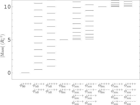
Figure 1: Absolute values of masses of 4D modes in the unit of $R_{5}^{-1}$, where $R_{6}=R_{5}/10$ is chosen.

The first KK mode appears at the energy scale $1/(2R_{5})$. These fields have the parities $(+-++)$ and $(-+++)$. When the energy scale is beyond $1/R_{5}$, the fields with the parity $(--++)$ as well as $(++++)$ become dynamical. Below the energy scale $1/(2R_{6})$, only the fields with the even parity with respect to the $x^{6}$ direction appear. These boundary conditions are $(++++)$, $(+-++)$, $(-+++)$ and $(--++)$.

On fixed lines, unbroken gauge group corresponds to the gauge transformation parameters which are nonzero under boundary conditions. Confined fields with representation of unbroken gauge group may be placed on the fixed lines. Let $(\phi(x,x^{5}))^{i_{1}\cdots i_{t}}_{j_{1}\cdots j_{s}}$ be a field with $t$ fundamental representation indices and $s$ fundamental conjugate representation indices with respect to SU($N$) on the fixed line $x^{6}=0$ or $x^{6}=\pi R_{6}$. Throughout this paper, we work with $N=1$ supersymmetry for 5D theory on fixed lines, which corresponds to $N=2$ in the 4D language. For $\phi$, the field $\phi^{c}$ is paired as its complex conjugate. Their boundary conditions are given by

$$(\phi(x,-x^{5}))^{i_{1}\cdots i_{t}}_{j_{1}\cdots j_{s}} \!\!\!=\!\!\! \eta_{1}(\hat{P}_{1})^{i_{1}}_{k_{1}}\cdots(\hat{P}_{1})^{i_{t}}_{k_{t}}(\phi(x,x^{5}))^{k_{1}\cdots k_{t}}_{l_{1}\cdots l_{s}}(\hat{P}_{1}^{\dagger})^{l_{1}}_{j_{1}}\cdots(\hat{P}_{1}^{\dagger})^{l_{t}}_{j_{t}},$$

$$(\phi^{c}(x,-x^{5}))_{i_{1}\cdots i_{t}}^{j_{1}\cdots j_{s}} \!\!\!=\!\!\! -\eta_{1}(\hat{P}_{1})^{j_{1}}_{l_{1}}\cdots(\hat{P}_{1})^{j_{s}}_{l_{s}}(\phi^{c}(x,x^{5}))_{k_{1}\cdots k_{t}}^{l_{1}\cdots l_{s}}(\hat{P}_{1}^{\dagger})^{k_{1}}_{i_{1}}\cdots(\hat{P}_{1}^{\dagger})^{k_{t}}_{i_{t}}.$$

$$(\phi(x,\pi R_{5}-x^{5}))^{i_{1}\cdots i_{t}}_{j_{1}\cdots j_{s}}, \!\!\!=\!\!\! \eta_{2}(\hat{P}_{2})^{i_{1}}_{k_{1}}\cdots(\hat{P}_{2})^{i_{t}}_{k_{t}}(\phi(x,\pi R_{5}+x^{5}))^{k_{1}\cdots k_{t}}_{l_{1}\cdots l_{s}}(\hat{P}_{2}^{\dagger})^{l_{1}}_{j_{1}}\cdots(\hat{P}_{2}^{\dagger})^{l_{t}}_{j_{t}},$$

$$(\phi^{c}(x,\pi R_{5}-x^{5}))_{i_{1}\cdots i_{t}}^{j_{1}\cdots j_{s}} \!\!\!=\!\!\! -\eta_{2}(\hat{P}_{2})^{j_{1}}_{l_{1}}\cdots(\hat{P}_{2})^{j_{s}}_{l_{s}}(\phi^{c}(x,\pi R_{5}+x^{5}))_{k_{1}\cdots k_{t}}^{l_{1}\cdots l_{s}}(\hat{P}_{2}^{\dagger})^{k_{1}}_{i_{1}}\cdots(\hat{P}_{2}^{\dagger})^{k_{t}}_{i_{t}},$$

where parity matrices with a hat over a symbol such as $\hat{P}_{1}$ indicate that they are projected parity matrices corresponding to the reduction of 6D unified gauge group to SU($N$). Here the parity of sign is $\eta_{1}=\pm 1$ and $\eta_{2}=\pm 1$. The boundary conditions for confined fields $\phi(x,x^{6})$ on fixed lines $x^{5}=0$ or $x^{5}=\pi R_{5}$ are defined in a parallel way. As a concrete example, for the parity matrices

$$\hat{P}_{1}=\left(\begin{array}[]{cc}{\bf 1}_{5}&\\ &-1\\ \end{array}\right),\qquad~{}\hat{P}_{2}=\left(\begin{array}[]{cc}{\bf 1}_{2}&\\ &-{\bf 1}_{4}\\ \end{array}\right),$$ (2.50)

the boundary conditions of several small representations in SU(6), the fundamental representation $\phi^{i}$, the two-rank antisymmetric representation $\phi^{ij}$ and the third-rank antisymmetric representation $\phi^{ijk}$, are tabulated in Table 2. All components can have zero modes. The origin of zero modes depends on $\hat{P}_{1}$, $\hat{P}_{2}$, $\eta_{1}$ and $\eta_{2}$.

Table 2: Boundary conditions of 6, 15 and 20 for the parity matrices (2.50). Here two signs in parentheses indicate the parities at $x^{5}=0$ and $x^{5}=\pi R_{5}$ in order.

Field	Component	Boundary condition
6 $\phi^{i}$	1,2	$(++)$	$(-+)$	$(+-)$	$(--)$
	3,4,5	$(+-)$	$(--)$	$(++)$	$(-+)$
	6	$(--)$	$(+-)$	$(-+)$	$(++)$
15 $\phi^{ij}$	12,34,35,45	$(++)$	$(-+)$	$(+-)$	$(--)$
	13,14,15,23,24,25	$(+-)$	$(--)$	$(++)$	$(-+)$
	16,26	$(--)$	$(+-)$	$(-+)$	$(++)$
	36,46,56	$(-+)$	$(++)$	$(--)$	$(+-)$
20 $\phi^{ijk}$	123,124,125,345	$(+-)$	$(--)$	$(++)$	$(-+)$
	126,346,356,456	$(--)$	$(+-)$	$(-+)$	$(++)$
	134,135,145,234,235,245	$(++)$	$(-+)$	$(+-)$	$(--)$
	136,146,156,236,246,256	$(-+)$	$(++)$	$(--)$	$(+-)$
$\eta_{1},\eta_{2}$		$1,1$	$-1,1$	$1,-1$	$-1,-1$

For example, the two components $1,2$ of 6 has zero mode for $\eta_{1}=\eta_{2}=1$, while the three components $3,4,5$ of 6 has zero mode for $\eta_{1}=-\eta_{2}=1$. Properties of the boundary conditions of the representations given in Table 2 will be used in explicit models analyzed later.

2.3 Couplings on fixed lines and points

Fields with the positive parity at fixed lines and fixed points of orbifold have nonzero values at the lines and points. These fields are coupled to fields confined on the fixed line and point. For a left-handed chiral superfield of fundamental representation denoted as $\Phi_{l}(x,x^{5})$ and its complex conjugate $\Phi_{l}^{c}(x,x^{5})$ confined on the fixed line $x^{6}=0$, the 6D fields have the interaction [14][17]

$$S_{5}=\int d^{6}x~{}\delta(x^{6})\left({1\over 2}\left[\Phi_{l}^{\dagger}e^{2V}\Phi_{l}+\Phi_{l}^{c}e^{-2V}\Phi_{l}^{c}{}^{\dagger}\right]_{D}+2\textrm{Re}\left[\left(\Phi^{c}_{l}(\partial_{5}+\Sigma_{5})\Phi_{l}\right)\right]_{F}\right).$$ (2.51)

The 5D fields $\Phi_{l}$ and $\Phi_{l}^{c}$ have the $\Lambda$-transformation

$$\Phi_{l}\to\Phi_{l}^{\prime}=e^{-\Lambda_{l}}\Phi_{l},~{}\quad\Phi_{l}^{c}\to\Phi_{l}^{c^{\prime}}=\Phi_{l}^{c}e^{\Lambda_{l}},$$ (2.52)

where $\Lambda(x,x^{5},x^{6}=0)=\Lambda_{l}(x,x^{5})$. The component action of (2.51) is given in Appendix B.1. The term $\int d^{6}x\delta(x^{6})2\textrm{Re}\left[\Phi^{c}_{l}(\partial_{5}+\Sigma_{5})\Phi_{l}\right]_{F}$ is invariant under $\Lambda$-transformation by itself. Similar terms appear also for other representations following properties of tensors in Eq.(LABEL:tensorp). The interaction of Eq.(2.51) is a gauge interaction. The gauge coupling constant appears in these equations when zero mode of 6D field is canonically normalized.

The 5D massless scalar field is expanded in terms of 4D mode as

$$\phi_{l}(x,x^{5})={1\over\sqrt{\pi R_{5}}}\left[\phi_{0}^{++}(x)+\sum_{n=1}^{\infty}\sqrt{2}\phi_{n}^{++}(x)\cos\left({nx^{5}\over R_{5}}\right)\right],$$ (2.53)

for the boundary condition $(++)$ in the orbifold property (LABEL:tensorp). The dimensionality of the field $\phi_{l}$ is defined as $\left[\phi_{l}\right]=\left[\textrm{mass}\right]^{3/2}$ which is different from the dimensionality of 6D fields and 4D fields confined on fixed points. In analogy to Table 1, 5D confined fields have the masses 0, $(n-{1\over 2})/R_{5}$, $n/R_{5}$ depending on boundary conditions.

We next consider interactions at fixed points. For a left-handed chiral superfield of fundamental representation denoted as $\Phi_{p}(x)$ confined on the fixed point $(x^{5},x^{6})=(0,0)$, the interactions of 6D fields with the fixed point field are

$$S_{4}=\int d^{6}x~{}\delta(x^{5})\delta(x^{6})\bigg{(}{1\over 2}\left[\Phi_{p}^{\dagger}e^{2V}\Phi_{p}\right]_{D}+2\textrm{Re}\left[f(\Phi_{p})\right]_{F}\bigg{)},$$ (2.54)

where the superpotential is denoted as $f(\Phi_{p})$. The $\Lambda$-transformation of $\Phi_{p}$ is given by

$$\Phi_{p}\to\Phi_{p}^{\prime}=e^{-\Lambda_{p}}\Phi_{p},$$ (2.55)

where $\Lambda(x,x^{5}=0,x^{6}=0)=\Lambda_{p}(x)$.

For the other fixed lines and points, $x^{5}=0$, $(x^{5},x^{6})=(\pi R_{5},0)$, $(0,\pi R_{6})$, $(\pi R_{5},\pi R_{6})$, the interactions of the 6D fields with fields of various representations on the fixed line and point can be obtained by the suitable replacements of delta functions and the operator $(\partial_{5}+\Sigma_{5})$.

2.4 Localization and decoupling of fields on fixed lines

We have written a 5D massless superfield for a field confined on a fixed line. A 5D massive superfield can be defined consistently with supersymmetry on the fixed line $x^{6}=0$ by adding to Eq.(2.51)

$$\int d^{6}x\delta(x^{6})\,2\textrm{Re}\left[M\epsilon(x^{5})\Phi_{l}^{c}\Phi_{l}\right]_{F}.$$ (2.56)

A parallel discussion can be made for 5D massive superfields on other fixed lines. Here the sign function is given by

$$\epsilon(x^{5})=\left\{\begin{array}[]{ccl}1&\textrm{for}&2z\pi R_{5}<x^{5}<(2z+1)\pi R_{5},\\ -1&\textrm{for}&(2z-1)\pi R_{5}<x^{5}<2z\pi R_{5},\\ 0&\textrm{for}&x^{5}=z\pi R_{5}.\\ \end{array}\right.$$ (2.60)

where $z$ is an integer.

From the 5D action obtained with Eqs.(B.3), (B.17) and (B.18), the scalar components of $\Phi_{l}$ and $\Phi_{l}^{c}$ are seen to obey

$$\left(\partial_{5}-M\epsilon\right)\left(\partial_{5}+M\epsilon\right)\phi_{l}=-M_{n}^{2}\phi_{l},\quad~{}\left(\partial_{5}+M\epsilon\right)\left(\partial_{5}-M\epsilon\right)\phi_{l}^{c}=-M_{n}^{2}\phi_{l}^{c},$$ (2.61)

where $M_{n}$ indicates the KK mass. The fermionic components have the same KK mass as $M_{n}$. With the mode expansion

$$\phi_{l}(x,x^{5})=\sum_{n=0}^{\infty}\phi_{n}(x)f_{n}(x^{5}),\quad~{}\phi_{l}^{c}(x,x^{5})=\sum_{n=0}^{\infty}\phi_{n}^{c}(x)g_{n}(x^{5}),$$ (2.62)

the equation (2.61) is equivalent to

$$\left(\partial_{5}+M\epsilon\right)f_{n}(x^{5})=M_{n}g_{n}(x^{5}),\quad~{}\left(-\partial_{5}+M\epsilon\right)g_{n}(x^{5})=M_{n}f_{n}(x^{5}).$$ (2.63)

The function $f_{0}$ and $g_{0}$ with $n=0$ are zero mode eigenfunction. The corresponding 4D fields $\phi_{0}$ and $\phi_{0}^{c}$ have zero mass $m_{0}=0$. For zero mode, the equations of motion for $f_{0}$ and $g_{0}$ is the two independent equations

$$\left(\partial_{5}+M\epsilon\right)f_{0}(x^{5})=0,\quad~{}\left(-\partial_{5}+M\epsilon\right)g_{0}(x^{5})=0.$$ (2.64)

From these equations, it is seen that the solutions have exponential forms which would lead to localization.

For the parity $(++)$ for $f_{0}$, the mode function is

$$f_{0}^{(++)}=\sqrt{M\over\sinh(\pi R_{5}M)}\times\left\{\begin{array}[]{c}e^{-M(|x^{5}|-\pi R_{5}/2)},~{}~{}~{}~{}~{}~{}~{}M>0,\\ e^{M(|x^{5}-\pi R_{5}|-\pi R_{5}/2)},~{}~{}~{}~{}M<0,\\ \end{array}\right.$$ (2.67)

for $0\leq x^{5}\leq\pi R_{5}$. The normalization constant is fixed by $\int_{0}^{\pi R_{5}}dx^{5}(f_{0}^{(++)})^{2}=1$. For $M>0$, $\phi_{l}^{++}$ is localized at $x^{5}=0$ and for $M<0$, it is localized at $x^{5}=\pi R_{5}$. For the parity $(--)$ for $f_{0}$, $f_{0}^{(--)}=0$. For the parity $(++)$ for $g_{0}$, the mode function is

$$g_{0}^{(++)}=\sqrt{M\over\sinh(\pi R_{5}M)}\times\left\{\begin{array}[]{c}e^{-M(|x^{5}-\pi R_{5}|-\pi R_{5}/2)},~{}~{}~{}~{}M>0,\\ e^{M(|x^{5}|-\pi R_{5}/2)},~{}~{}~{}~{}~{}~{}~{}~{}~{}~{}~{}~{}M<0,\\ \end{array}\right.$$ (2.70)

for $0\leq x^{5}\leq\pi R_{5}$. The normalization constant is fixed by $\int_{0}^{\pi R_{5}}dx^{5}(g_{0}^{(++)})^{2}=1$. For $M>0$, $\phi_{l}^{c++}$ is localized at $x^{5}=\pi R_{5}$ and for $M<0$, it is localized at $x^{5}=0$. For the parity $(--)$ for $g_{0}$, $g_{0}^{(--)}=0$. These mean that the fields $\phi_{l}^{++}$ and $\phi_{l}^{c++}$ are localized at the opposite fixed points. The product $f_{0}^{(++)}g_{0}^{(++)}$ is written as

$$f_{0}^{(++)}g_{0}^{(++)}={M\over\sinh(\pi R_{5}M)},$$ (2.71)

on the fixed line $0\leq x^{5}\leq\pi R_{5}$ for arbitrary $M$ (including $M=0$).

The $n$-th eigenfunction $f_{n}$ is related to the function $g_{n}$ with the opposite parities. For the parity $(++)$ for $f_{n}$ and $(--)$ for $g_{n}$, the functions are

$$f_{n}^{(++)}=\sqrt{2\over\pi R_{5}}\cos\left({n\over R_{5}}x^{5}\right),\quad~{}g_{n}^{(--)}=\sqrt{2\over\pi R_{5}}\sin\left({n\over R_{5}}x^{5}+\Omega_{n}\right),$$ (2.72)

where $\tan\Omega_{n}=-MR_{5}/n$. The corresponding 4D modes $\phi_{n}^{(++)}$ and $\phi_{n}^{c(--)}$ have the mass squared $M_{n}^{2}=M^{2}+(n/R_{5})^{2}$ . The functions $f_{n}^{(--)}$ and $g_{n}^{(++)}$ are

$$f_{n}^{(--)}=\sqrt{2\over\pi R_{5}}\sin\left({n\over R_{5}}x^{5}-\Omega_{n}\right),\quad~{}g_{n}^{(++)}=\sqrt{2\over\pi R_{5}}\cos\left({n\over R_{5}}x^{5}\right).$$ (2.73)

The 4D modes $\phi_{n}^{(--)}$ and $\phi_{n}^{c(++)}$ have the mass squared $M_{n}^{2}=M^{2}+(n/R_{5})^{2}$. The other eigenfunctions are given by $f_{n}^{(+-)}=f_{n+1/2}^{(++)}$, $g_{n}^{(-+)}=g_{n+1/2}^{(--)}$, $f_{n}^{(-+)}=f_{n+1/2}^{(--)}$ and $g_{n}^{(+-)}=g_{n+1/2}^{(++)}$. The 4D modes $\phi_{n}^{(+-)}$, $\phi_{n}^{c(-+)}$, $\phi_{n}^{(-+)}$ and $\phi_{n}^{c(+-)}$ have the mass squared $M_{n}^{2}=M^{2}+((n+1/2)/R_{5})^{2}$. The 4D KK modes of fixed-line fields with 5D masses are heavier than the KK modes of the corresponding 5D massless fields.

Fixed-point couplings for heavy fields

We have seen that zero mode arises from fixed-line fields with and without 5D mass terms. In contrast, 4D heavy modes yield if 4D interactions are added.

Here for the 5D superfield $\Phi_{l}^{c}(x,x^{5})$ with the scalar component $\phi_{l}^{c}$ of dimensionality $\left[\phi_{l}^{c}\right]=\left[\textrm{mass}\right]^{3/2}$ and the 4D superfield $\Phi_{p}(x)$ with the scalar component $\phi_{p}$ of dimensionality $\left[\phi_{p}\right]=\left[\textrm{mass}\right]$, we consider the fixed-point coupling

$$\delta(x^{5})\delta(x^{6})(2\textrm{Re}[\sqrt{m_{\textrm{\scriptsize dec}}}\Phi_{l}^{c}\Phi_{p}]_{F}+{1\over 2}[\Phi_{p}^{\dagger}e^{2V}\Phi_{p}]_{D}),$$ (2.74)

which is still supersymmetric. If $\Phi_{l}^{c}$ has a 5D mass, the mass is taken as positive so that the coupling (2.74) is made on the fixed point where $\Phi_{l}^{c}$ is localized. After integration of auxiliary fields, the supersymmetric mass terms are obtained as

$${\cal L}_{\textrm{\scriptsize mass}}=\delta(x^{5})\delta(x^{6})\left(-m_{\textrm{\scriptsize dec}}\delta(x^{5})\phi_{p}\phi_{p}^{*}-m_{\textrm{\scriptsize dec}}\phi_{l}^{c}\phi_{l}^{c*}+(\textrm{fermions})\right).$$ (2.75)

For a large $m_{\textrm{\scriptsize dec}}$, the 4D mode $\phi_{p}(x)$, $\phi_{l}^{c\,++}(x)$ and their superpartners become heavy.

One could introduce Chern-Simons terms on 5D fixed lines. Such terms are relevant to anomalies in 5D localized on fixed points [18]. We will not treat this issue further in the paper.

3 High energy behavior of gauge couplings

Employing the action defined above, we will consider 6D SU(6) models where zero mode is composed of right-handed neutrino and their superpartners as well as the field content of MSSM. Before moving on to explicit models, we give the approach to examine high energy behavior of gauge couplings. The characteristic scales of theory are the radii $R_{5}$ and $R_{6}$ and the cutoff of 6D theory $M_{s}$. Since we assume $R_{5}>R_{6}$, it is needed to deal with effective field theory at energy scales from $1/(2R_{5})$ to $1/(2R_{6})$. Here $1/(2R_{5})$ is the minimum mass of KK mode obtained from Table 1 and from discussion of 5D massless fields below (2.53) and of 5D massive fields, whereas $1/(2R_{6})$ is the mass when the $x^{6}$ direction appears. Our approach is based on 4D KK effective Lagrangian [19][20]. Although higher-dimensional theory is non-renormalizable, it can be assumed that the contributions from the KK states with masses larger than the scale of interest are decoupled from the theory. In this approximation the corrections to the gauge couplings can be calculated. The first KK excitation occurs at the scale $1/(2R_{5})$. Up to this scale the gauge coupling evolution has a contribution only from zero mode. Between $1/(2R_{5})$ and $1/R_{5}$ (to avoid complexity the discussion is presented for the masses listed in Table 1 or for the moment we assume that the absolute values of 5D masses $|M|$ is zero or larger than $1/(2R_{6})$), the running is still logarithmic but beta functions are modified due to the first KK excitation. Whenever a KK threshold is crossed, beta functions are renewed. Gauge couplings are described as functions of the energy, depending on the number of KK states.

We consider gauge field Lagrangian

$${\cal L}_{\textrm{\scriptsize gauge}}=-{1\over 4g^{2}}(F_{MN}^{a})^{2},$$ (3.1)

from the action (2.17). The gauge field for the parity $(++++)$ is decomposed as in Eq.(2.44),

$$A_{m}^{a}(x,x^{i})=A_{m}^{a}{}_{(00)}^{++++}(x)+\sum_{n=1}\sqrt{2}A_{m}^{a}{}_{(n0)}^{++++}(x)\cos\left({nx^{5}\over R_{5}}\right)$$

$$~{}+\sum_{n=1}\sqrt{2}A_{m}^{a}{}_{(0n)}^{++++}(x)\cos\left({nx^{6}\over R_{6}}\right)+\sum_{n=1}\sum_{m=1}2A_{m}^{a}{}_{(nm)}^{++++}(x)\cos\left({nx^{5}\over R_{5}}\right)\cos\left({mx^{6}\over R_{6}}\right).$$ (3.2)

The mode expansions for $(+-++)$, $(--++)$ and $(-+++)$ are obtained similarly to (C.2), (C.5) and (C.6). The 5-component and 6-component of gauge field corresponding to (3.2) have the parities $(--++)$ and $(++--)$, respectively. They are given by

$$A_{5}^{a}(x,x^{i}) \!\!\!=\!\!\! \sum_{n=1}\sqrt{2}A_{5}^{a}{}_{(n0)}^{--++}(x)\sin\left({nx^{5}\over R_{5}}\right)+\sum_{n=1}\sum_{m=1}2A_{5}^{a}{}_{(nm)}^{--++}(x)\sin\left({nx^{5}\over R_{5}}\right)\cos\left({mx^{6}\over R_{6}}\right),$$

$$A_{6}^{a}(x,x^{i}) \!\!\!=\!\!\! \sum_{m=1}\sqrt{2}A_{6}^{a}{}_{(0m)}^{++--}(x)\sin\left({mx^{6}\over R_{6}}\right)+\sum_{n=1}\sum_{m=1}2A_{6}^{a}{}_{(nm)}^{++--}(x)\cos\left({nx^{5}\over R_{5}}\right)\sin\left({mx^{6}\over R_{6}}\right).$$

We keep only the mode $(++)$ with respect to $x^{6}$, since we have interest in states with masses less than $1/(2R_{6})$. Substituting the KK mode expansion into the Lagrangian (3.1), we obtain the 4D gauge part Lagrangian

$$\int_{0}^{\pi R_{5}}dx^{5}\int_{0}^{\pi R_{6}}dx^{6}~{}{\cal L}_{\textrm{\scriptsize gauge}}$$ (3.4)

$$\!\!=\!\! -{\pi^{2}R_{5}R_{6}\over 4g^{2}}(F_{mn}^{a}{}_{(0)})^{2}$$

$$-{\pi^{2}R_{5}R_{6}\over 4g^{2}}\sum_{n=1}\left((F_{mn}^{a}{}_{(n)})^{2}+2f^{abc}F_{mn}^{a}{}_{(0)}A^{mb}{}_{(n)}A^{nc}{}_{(n)}+2F_{m5}^{a}{}_{(n)}F^{m5a}_{(n)}\right).$$

For notational simplicity, we have defined $A_{m}^{a}{}_{(0)}(x)\equiv A_{m}^{a}{}_{(00)}^{++++}(x)$, $A_{m}^{a}{}_{(n)}(x)\equiv A_{m}^{a}{}_{(n0)}^{++++}(x)$, $A_{5}^{a}{}_{(n)}(x)\equiv A_{5}^{a}{}_{(n0)}^{--++}(x)$. The field strengths are given by

$$F_{mn}^{a}{}_{(0)} \!\!=\!\! \partial_{m}A_{n}^{a}{}_{(0)}-\partial_{n}A_{m}^{a}{}_{(0)}+f^{abc}A_{m}^{b}{}_{(0)}A_{n}^{c}{}_{(0)},$$

$$F_{mn}^{a}{}_{(n)} \!\!=\!\! \partial_{m}A_{n}^{a}{}_{(n)}-\partial_{n}A_{m}^{a}{}_{(n)}+f^{abc}A_{m}^{b}{}_{(m)}A_{n}^{c}{}_{(r)}\delta_{nmr}^{+}+f^{abc}(A_{m}^{b}{}_{(0)}A_{n}^{c}{}_{(n)}-A_{n}^{b}{}_{(0)}A_{m}^{c}{}_{(n)}),$$

$$F_{m5}^{a}{}_{(n)} \!\!=\!\! \partial_{m}A_{5}^{a}{}_{(n)}+(\textrm{${n\over R_{5}}$})A_{m}^{a}{}_{(n)}+f^{abc}A_{m}^{b}{}_{(m)}A_{5}^{c}{}_{(r)}\delta_{nmr}^{-}+f^{abc}A_{m}^{b}{}_{(0)}A_{5}^{c}{}_{(n)},$$

with $\delta_{nmr}^{\pm}=(\delta_{n,m+r}+\delta_{m,n+r}\pm\delta_{r,n+m})/\sqrt{2}$. The $n$-th KK gauge field begins to play a dynamical role at energy scales higher than $(n/R_{5})$. We treat the summation over KK modes in the Lagrangian (3.4) as scale-dependent. This is explicitly written as $\sum_{n=1}^{m}$ at the energy range $m/R_{5}\leq E<(m+1)/R_{5}$. At scales less than $1/(2R_{5})$, the Lagrangian describes only zero mode as the summation is simply zero. The $n$-th KK scalar $A_{5}^{a}{}_{(n)}$ has the same mass as that of the $n$-th KK gauge field, as more explicitly seen after gauge fixing. The summation over the KK modes is treated similarly to the KK gauge field case.

The 4D gauge couplings are obtained as

$${1\over g_{4D}^{2}}={\pi^{2}R_{5}R_{6}\over g^{2}}+\cdots={(\pi R_{5}M_{s})(\pi R_{6}M_{s})\over\hat{g}^{2}}+\cdots,$$ (3.6)

where a dimensionless coupling constant is defined as $\hat{g}=M_{s}g$. Here the ellipses denote possible contributions of fixed-line and fixed-point kinetic terms. If dimensionless gauge coupling constants with the origins in 6D, 5D and 4D are of the same order, the first terms in Eq.(3.6) would dominate due to the volume suppression $1>(R_{6}M_{s})^{-1}>(R_{5}M_{s})^{-1}$. However, in the expression (3.6), there is subtlety. If $M_{s}=10^{18}$GeV, $1/R_{6}=4\times 10^{17}$GeV, $1/R_{5}=4\times 10^{16}$GeV and $g_{4D}\sim 1$ are chosen, the dimensionless gauge coupling constants are of order of $\hat{g}\sim(100\pi)\times(10\pi)\gg 1$. It seems unnatural that $\hat{g}$ is larger than 1 since it is made dimensionless with the cutoff $M_{s}$. To obtain $\hat{g}\sim 1$ naturally, taking into account geometric loop factor may be viable [13]. We here simply ignore the contributions of fixed-line and fixed-point terms.

The 4D Lagrangian (3.4) is invariant under a standard 4D gauge transformation. The infinitesimal gauge transformation law for $A_{m}^{a}{}_{(0)}$ is given by

$$\delta A_{m}^{a}{}_{(0)}=\partial_{m}\alpha^{a}+f^{abc}A_{m}^{b}{}_{(0)}\alpha^{c}$$ (3.7)

where $\alpha^{a}(x)$ is an infinitesimal parameter dependent on 4D coordinates. The KK gauge field and scalar are transformed as adjoint matter fields,

$$\delta A_{m}^{a}{}_{(n)} \!\!=\!\! f^{abc}A_{m}^{b}{}_{(n)}\alpha^{c},$$ (3.8)

$$\delta A_{5}^{a}{}_{(n)} \!\!=\!\! f^{abc}A_{5}^{b}{}_{(n)}\alpha^{c}.$$ (3.9)

In addition to the standard gauge invariance, the Lagrangian (3.4) is also invariant under another gauge transformation with the infinitesimal local parameter $\alpha^{a}_{(n)}(x)$,

$$\delta_{(n)}A_{m}^{a}{}_{(0)}=0,$$ (3.10)

$$\delta_{(n)}A_{m}^{a}{}_{(n)}=\partial_{m}\alpha^{a}_{(n)}+f^{abc}A_{m}^{b}{}_{(m)}\alpha^{c}_{(r)}\delta_{nmr}^{+}+f^{abd}A_{m}^{b}{}_{(0)}\alpha^{c}_{(n)},$$ (3.11)

$$\delta_{(n)}A_{5}^{a}{}_{(n)}=-({n\over R_{5}})\alpha_{(n)}^{a}+f^{abc}A_{5}^{b}{}_{(m)}\alpha^{c}_{(r)}\delta_{nmr}^{-}.$$ (3.12)

For these two kinds of gauge invariance, a version of the generalized Lorenz gauge convenient for the background field method can be chosen [20]. It is straightforward to include part of fermion and scalar fields as well as the other boundary conditions $(+-++)$, $(--++)$ and $(-+++)$.

We now give gauge coupling constants in such a way to track the number of KK modes. For scales less than the mass of the first KK mode, the gauge coupling constant is given in terms of $\alpha^{-1}\equiv 4\pi g^{-2}(\pi^{2}R_{5}R_{6})$ by

$$\alpha^{-1}(\mu)=\alpha^{-1}(M)+{b\over 2\pi}\log{M\over\mu},~{}\quad\textrm{for}~{}~{}\mu<{1\over 2R_{5}},$$ (3.13)

where $\mu$ and $M$ are the scale of interest and another scale. In Eq.(3.13), $b$ is obtained only from zero mode part as

$$b=-\!\sum_{\textrm{\scriptsize gauge}}\!{11\over 3}C_{2}(G)+\sum_{\textrm{\scriptsize Weyl}}{2\over 3}C(r)+\!\!\!\!\sum_{\textrm{\scriptsize\begin{tabular}[]{c}complex\\ scalar\end{tabular}}}\!\!\!\!{1\over 3}C(r),$$ (3.16)

with the quadratic Casimir operator for the adjoint representation $C_{2}(G)=N$ and the coefficient in the trace of the product of two generator matrices $C(r)={1\over 2}$. In the factor $11/3$ for gauge, the contributions of the corresponding ghost fields have been included. As scales cross the mass of the first KK excitation, the first KK mode becomes dynamical. Then $\alpha^{-1}$ is given by

$$\alpha^{-1}(\mu)=\alpha^{-1}(M)+{b\over 2\pi}\log{M\over\mu}+{b_{(1)}\over 2\pi}\log{1\over 2\mu R_{5}},~{}\quad\textrm{for}~{}~{}{1\over 2R_{5}}\leq\mu<{1\over R_{5}},$$ (3.17)

where

$$b_{(1)}=-\!\sum_{\textrm{\scriptsize gauge}}\!{11\over 3}C(r)+\sum_{\textrm{\scriptsize Dirac}}{4\over 3}C(r)+\!\!\!\!\sum_{\textrm{\scriptsize\begin{tabular}[]{c}complex\\ scalar\end{tabular}}}\!\!\!\!{1\over 3}C(r),$$ (3.20)

When the second KK mode becomes dynamical, $\alpha^{-1}$ is given by

$$\alpha^{-1}(\mu)=\alpha^{-1}(M)+{b\over 2\pi}\log{M\over\mu}+{b_{(1)}\over 2\pi}\log{1\over 2\mu R_{5}}+{b_{(2)}\over 2\pi}\log{1\over\mu R_{5}},$$ (3.21)

for $1/R_{5}\leq\mu<3/(2R_{5})$, where

$$b_{(2)}=-\!\!\sum_{\textrm{\scriptsize gauge}}\!{11\over 3}C_{2}(G)+\sum_{\textrm{\scriptsize Dirac}}{4\over 3}C(r)+\!\!\!\!\sum_{\textrm{\scriptsize\begin{tabular}[]{c}complex\\ scalar\end{tabular}}}\!\!\!\!{1\over 3}C(r).$$ (3.24)

In the equations (3.20) and (3.24), the coefficients of gauge part are different from each other. The gauge part of $b_{(1)}$ appears from coset and it gives $C(r)$, whereas the gauge part of $b_{(2)}$ is the contribution of group and it gives $C_{2}(G)$ which is the same as that of zero mode. If every mass is given in $n/(2R_{5})$, a generic $\alpha^{-1}$ is given by

$$\alpha^{-1}(\mu)=\alpha^{-1}(M)+{b\over 2\pi}\log{M\over\mu}+\sum_{s=1,2}{b_{(s)}\over 2\pi}\left[(n+1-s)\log{1\over 2\mu R_{5}}+\log((2n-s)!!)\right],$$ (3.25)

for $(n-1/2)/R_{5}\leq\mu<n/R_{5}$ and

$$\alpha^{-1}(\mu)=\alpha^{-1}(M)+{b\over 2\pi}\log{M\over\mu}+\sum_{s=1,2}{b_{(s)}\over 2\pi}\left[n\log{1\over 2\mu R_{5}}+\log((2n-2+s)!!)\right],$$ (3.26)

for $n/R_{5}\leq\mu<(n+1/2)/R_{5}$.

4 Model with Higgs as 5D multiplets

We consider two cases where Higgs fields are 5D chiral superfields and they are a part of the 6D gauge multiplet. In this section, we consider a model where Higgs fields are 5D chiral superfields as a version with gaugino-mediated supersymmetry breaking of the model [7].

The starting parity matrices are given by

$$P_{1}=P_{3}={\bf 1}_{6},\quad~{}P_{2}=\left(\begin{array}[]{cc}{\bf 1}_{2}&\\ &-{\bf 1}_{4}\\ \end{array}\right),\quad~{}P_{4}=\left(\begin{array}[]{ccccc|c}{\bf 1}_{5}&\\ &-1\\ \end{array}\right),$$ (4.5)

for the boundary conditions (LABEL:parityg5) and (LABEL:parityg6). The vector superfield $V(A_{m},\lambda)$ has the boundary conditions

$$\left(\begin{array}[]{cc|ccc|c}_{(++++)}&{}_{(++++)}&{}_{(+-++)}&{}_{(+-++)}&{}_{(+-++)}&{}_{(+-+-)}\\ _{(++++)}&{}_{(++++)}&{}_{(+-++)}&{}_{(+-++)}&{}_{(+-++)}&{}_{(+-+-)}\\ \hline\cr_{(+-++)}&{}_{(+-++)}&{}_{(++++)}&{}_{(++++)}&{}_{(++++)}&{}_{(+++-)}\\ _{(+-++)}&{}_{(+-++)}&{}_{(++++)}&{}_{(++++)}&{}_{(++++)}&{}_{(+++-)}\\ _{(+-++)}&{}_{(+-++)}&{}_{(++++)}&{}_{(++++)}&{}_{(++++)}&{}_{(+++-)}\\ \hline\cr_{(+-+-)}&{}_{(+-+-)}&{}_{(+++-)}&{}_{(+++-)}&{}_{(+++-)}&{}_{(++++)}\\ \end{array}\right).$$ (4.12)

The zero mode $(++++)$ is in the blocks of square matrices of rank 2, 3 and 1. Among these zero mode components, the blocks of the square matrices of rank 2 and 3 have the unbroken gauge group SU(3)$\times$SU(2)$\times$U(1) which is identified as SU(3)${}_{\textrm{\scriptsize C}}$$\times$SU(2)${}_{\textrm{\scriptsize W}}$$\times$U(1)_Y. This gives the correct normalization for hypercharges. The SU(5) relation for the three MSSM gauge coupling constants is obtained and the successful prediction of the MSSM for $\sin^{2}\theta_{w}$ is recovered. The other block has extra U(1) gauge group which we write as U(1)^′. In the up-left corner the components of square matrix of rank 5 have the positive parity in the $x^{6}$ direction and all of them contributes to dynamics at scales less than $1/(2R_{5})$. For each fixed line and point, an unbroken gauge group of restricted gauge symmetry and the number of supersymmetry in the 4D language are tabulated in Table 3.

Table 3: Gauge groups and supersymmetries $N$ on fixed lines and points.

Location	Gauge group	$N$	Location	Gauge group	$N$
$x^{6}=0$	SU(6)	2	$(0,0)$	SU(6)	1
$x^{6}=\pi R_{6}$	SU(5)$\times$U(1)′	2	$(0,\pi R_{6})$	SU(5)$\times$U(1)′	1
$x^{5}=0$	SU(6)	2	$(\pi R_{5},0)$	SU(4)$\times$SU(2)$\times$U(1)	1
$x^{5}=\pi R_{5}$	SU(4)$\times$SU(2)$\times$U(1)	2	$(\pi R_{5},\pi R_{6})$	SU(3)$\times$SU(2)$\times$U(1)$\times$U(1)′	1

The gauge supersymmetry and supersymmetry at each fixed point are given by the intersection of those on the adjacent fixed lines; for example, SU(3)$\times$SU(2)$\times$U(1)$\times$U(1)^′ $=$ SU(5)$\times$U(1)^′ $\cap$ SU(4)$\times$SU(2)$\times$U(1).

The charges for U(1) and U(1)^′ are defined in a similar way to case of the 4D SU(5). The three independent diagonal matrices invariant under SU(3) are

$$\textrm{diag}(1,-1,0,0,0,0),\quad\textrm{${1\over\sqrt{15}}$}\,\textrm{diag}(1,1,1,1,1,-5),\quad\textrm{${1\over\sqrt{15}}$}\,\textrm{diag}(3,3,-2,-2,-2,0).$$ (4.13)

In the notation of Appendix A.1, they are $\lambda_{3}$, $\lambda_{35}$ and $(\textrm{${\sqrt{5}\over 3}$}\lambda_{8}+\textrm{${\sqrt{10}\over 3}$}\lambda_{15}+\textrm{${\sqrt{6}\over 6}$}\lambda_{24})$, respectively. For the electric charge after SU(2)${}_{\textrm{\scriptsize W}}$$\times$U(1)_Y is broken to U(1)${}_{\textrm{\scriptsize em}}$, the charge matrix of U(1)${}_{\textrm{\scriptsize em}}$ is

$$Q \!\!\!=\!\!\! T_{3}+Y=\textrm{${1\over 2}$}\lambda_{3}+\textrm{${1\over 2}$}\textrm{${\sqrt{15}\over 3}$}(\textrm{${\sqrt{5}\over 3}$}\lambda_{8}+\textrm{${\sqrt{10}\over 3}$}\lambda_{15}+\textrm{${\sqrt{6}\over 6}$}\lambda_{24})=\textrm{diag}(1,0,\textrm{$-{1\over 3}$},\textrm{$-{1\over 3}$},\textrm{$-{1\over 3}$},0).$$ (4.14)

From the other independent diagonal matrix in Eq.(4.13), we take the charge matrix for U(1)^′ as

$$Q_{\textrm{\scriptsize x}} \!\!\!=\!\!\! 3\sqrt{15}\,p\lambda_{35}=3p\,\textrm{diag}(1,1,1,1,1,,-5),$$ (4.15)

where $p$ is a constant. For the fixed lines with unbroken SU(5)$\times$U(1)^′, the U(1)^′ is not quantized, whereas the U(1)_Y in SU(5) is quantized.

In the gauge multiplet, the superfield $\Sigma_{5}(\sigma_{5},\lambda_{5})$ has the boundary condition,

$$\left(\begin{array}[]{cc|ccc|c}_{(--++)}&{}_{(--++)}&{}_{(-+++)}&{}_{(-+++)}&{}_{(-+++)}&{}_{(-++-)}\\ _{(--++)}&{}_{(--++)}&{}_{(-+++)}&{}_{(-+++)}&{}_{(-+++)}&{}_{(-++-)}\\ \hline\cr_{(-+++)}&{}_{(-+++)}&{}_{(--++)}&{}_{(--++)}&{}_{(--++)}&{}_{(--+-)}\\ _{(-+++)}&{}_{(-+++)}&{}_{(--++)}&{}_{(--++)}&{}_{(--++)}&{}_{(--+-)}\\ _{(-+++)}&{}_{(-+++)}&{}_{(--++)}&{}_{(--++)}&{}_{(--++)}&{}_{(--+-)}\\ \hline\cr_{(-++-)}&{}_{(-++-)}&{}_{(--+-)}&{}_{(--+-)}&{}_{(--+-)}&{}_{(--++)}\\ \end{array}\right).$$ (4.22)

The boundary conditions of $\Sigma_{5}$ also has the positive parity in the $x^{6}$ direction in the blocks of square matrices of rank 5 and 1. Thus $\Sigma_{5}$ has dynamical components below $1/(2R_{6})$. The superfields $\Phi$ and $\Sigma_{6}$ also propagate in 6D, in addition to $V$ and $\Sigma_{5}$. The components for $\Sigma_{6}$ and $\Phi$ are seen to be non-dynamical until $1/(2R_{6})$. The boundary conditions for $\Sigma_{6}$ and $\Phi$ are explicitly given in Appendix C.2.

We take confined fields on fixed lines and points as matter. The field content is shown in Table 4 with a consideration similar to that in obtaining explicit boundary conditions given in Table 2.

Table 4: Field content added to the gauge multiplet $(V,\Sigma_{5},\Sigma_{6},\Phi)(x,x^{5},x^{6})$ in the model with Higgs multiplets on a fixed line. Quantum numbers are shown for gauge groups of the restricted gauge symmetry on each fixed line or point. For $(\Psi_{\imath},\Psi_{\imath}^{c})$, the parity of sign should be regarded as not $\eta_{1},\eta_{2}$ but the correspondent in the $x^{6}$ direction. Here $\imath=1,2$, $\jmath=1,2,3$.

Location	Field	Quantum number		$\eta_{1}$	$\eta_{2}$
$x^{6}=\pi R_{6}$	$(H_{1},H_{1}^{c})(x,x^{5})$	$(5^{*},2p)$	$\in$ SU(5)$\times$U(1)′	1	1
	$(H_{2},H_{2}^{c})(x,x^{5})$	$(5,-2p)$		1	1
	$(T_{\imath},T_{\imath}^{c})(x,x^{5})$	$(10,p)$		1	$-1$
	$(T^{\prime}_{\imath},T_{\imath}^{{}^{\prime}c})(x,x^{5})$	$(10,p)$		1	1
$(0,\pi R_{6})$	$T_{3}(x)$	$(10,p)$	$\in$ SU(5)$\times$U(1)′	—
	$N_{\jmath}(x)$	$(1,5p)$		—
$x^{5}=0$	$(\Psi_{\jmath},\Psi_{\jmath}^{c})(x,x^{6})$	$6^{*}$	$\in$ SU(6)	1	1
$(\pi R_{5},0)$	$S(x)$	$(1,1,0)$	$\in$ SU(4)$\times$SU(2)$\times$U(1)	—

For all fields on fixed lines in this model, 5D masses are zero. In our notation, a conjugated field has the opposite transformation property with the non-conjugated field, and we specify the transformation property of a hypermultiplet by that of the non-conjugated chiral superfield; for instance, $H_{1}$ and $H_{1}^{c}$ transforms as $(5^{*},2p)$ and $(5,-2p)$ under SU(5)$\times$U(1)^′, respectively. The superfields $T$, $T^{\prime}$ and $\Psi$ has Yukawa coupling at the fixed point $(x^{5},x^{6})=(0,\pi R_{6})$. In order to avoid the fermion mass relation for the first two generations, $T_{\imath}$, $T_{\imath}^{c}$, $T_{\imath}^{\prime}$ and $T_{\imath}^{{}^{\prime}c}$ propagate in 5D. For the third generation, $T_{3}$ is set at the intersection fixed point $(x^{5},x^{6})=(0,\pi R_{6})$ to give the approximate mass relation for $m_{\tau}/m_{b}$ in SU(5), for example, if down-type quarks and charged leptons have small mixing angles in flavor space. The superfield $S$ confined at $(x^{5},x^{6})=(\pi R_{5},0)$ develops $\theta\theta F_{s}$. This field is directly coupled to the gauge multiplet only. It originates gaugino-mediated supersymmetry breaking.

The charges of U(1)^′ for confined fields are assigned so as to allow the Yukawa interactions

$$TTH_{2},\quad~{}T\Psi H_{1},$$ (4.23)

where the ${\bf 5}^{*}$-part of the whole ${\bf 6}^{*}$ of $\Psi$ contributes to the coupling. From Eq.(4.15), $H_{1}$, $H_{2}$ and $T$ have the U(1)^′ charges $2p$, $-2p$ and $p$, respectively as shown in Table 4, where we have assumed $H_{1}$ and $H_{2}$ have the opposite U(1)^′ charges. The zero modes $(++++)$ of the vector multiplet and $(++)$ of matter multiplets contribute to 4D chiral anomaly. The SU(3)$\times$SU(2)$\times$U(1) part is clearly anomaly free because zero mode is composed of right-handed neutrinos and their superpartners as well as the field content of MSSM. The part of U(1)^′ should be checked. The zero modes of $H_{\imath}$, $T_{\imath}$, $T_{\imath}^{\prime}$, $\Psi_{\jmath}$ ($\imath=1,2$, $\jmath=1,2,3$) and their charge conjugate as well as $T_{3}$ contribute

$$0+3\times 10\times p+3\times 5\times(-3p) \!\!\!=\!\!\! -3(5p)\qquad~{}~{}\textrm{to}~{}\textrm{Tr}\,Q_{\textrm{\scriptsize x}},$$ (4.24)

$$0+3\times 3\times p+3\times 1\times(-3p) \!\!\!=\!\!\! 0\qquad\qquad\quad~{}\textrm{to}~{}\textrm{Tr}_{\textrm{\scriptsize SU(2)}}\,Q_{\textrm{\scriptsize x}},$$ (4.25)

$$0+3\times(p+2p)+3\times(-3p) \!\!\!=\!\!\! 0\qquad\qquad\quad~{}\textrm{to}~{}\textrm{Tr}_{\textrm{\scriptsize SU(3)}}\,Q_{\textrm{\scriptsize x}},$$ (4.26)

$$0+3\times 10\times p^{3}+3\times 5\times(-3p)^{3} \!\!\!=\!\!\! -3(125p^{3})\quad~{}\textrm{to}~{}\textrm{Tr}\,Q_{\textrm{\scriptsize x}}^{3}.$$ (4.27)

The SU(5) singlets $N_{\jmath}~{}(\jmath=1,2,3)$ with the U(1)^′ charge $5p$ confined on the fixed point $(x^{5},x^{6})=(0,\pi R_{6})$ cancel the contributions given above to the anomalous terms.

The gauge symmetry for U(1)^′ is broken via the coupling

$$\delta(x^{5})\delta(x^{6}-\pi R_{6})\,2\textrm{Re}\left[X(B\bar{B}-\Lambda_{\textrm{\scriptsize x}}^{2})\right]_{F},$$ (4.28)

where $X$, $B$ and $\bar{B}$ confined on the fixed point have the quantum number $(1,0)$, $(1,10p)$ and $(1,-10p)$ under SU(5)$\times$U(1)^′, respectively. A dimensionful constant is denoted as $\Lambda_{\textrm{\scriptsize x}}$. The U(1)^′ is broken by the vacuum expectation value

$$\langle B\rangle=\langle\bar{B}\rangle=\Lambda_{\textrm{\scriptsize x}}.$$ (4.29)

Adding the coupling $\delta(x^{5})\delta(x^{6}-\pi R_{6})2\textrm{Re}\left[\bar{B}N_{\jmath}N_{\jmath}\right]_{F}$ to Eq.(4.28) induces Majorana mass of right-handed neutrino.

4.1 Mass spectrum

Here we give quantum numbers for components of zero modes and KK modes of the 6D gauge multiplet and the fields given in Table 4. In the 6D gauge multiplet, the vector superfield $V$ has zero mode. They give one vector and one two-component Weyl fermion. Each 4D chiral superfield has one complex scalar and one two-component Weyl fermion. Each pair of 5D superfields, collectively ($\Phi_{l},\Phi_{l}^{c}$), contributes to one complex scalar and one two-component Weyl fermion. Because $S$ is a spurion, it does not have zero mode nor KK modes. The massless mode is the right-handed neutrino and its superpartner as well as the field content of MSSM with two Higgs fields. Representations under SU(3)${}_{\textrm{\scriptsize C}}$ $\times$SU(2)W$\times$U(1)_Y are tabulated in Table 5.

Table 5: Quantum numbers for SU(3)${}_{\textrm{\scriptsize C}}$$\times$SU(2)${}_{\textrm{\scriptsize W}}$$\times$U(1)_Y of zero mode for superfields given in Table 4 and the gauge multiplet. The notation for zero-mode quarks and leptons is also shown. The superfields $\Sigma_{5},\Sigma_{6},\Phi,H_{\imath}^{c},T_{\imath}^{c},T_{\imath}^{\prime}{}^{c},\Psi_{j}^{c},S$ do not have zero mode. Here $\imath=1,2$, $\jmath=1,2,3$.

$V(x,x^{5},x^{6})$	$(1,3,0)\oplus(8,1,0)$	Zero-mode
$H_{1}(x,x^{5})$	$(1,2,-1/2)$	quark and
$H_{2}(x,x^{5})$	$(1,2,1/2)$	lepton
$T_{\imath}(x,x^{5})$	$(3,2,1/6)$	${1\over\sqrt{\pi R_{5}}}$$q_{\imath}(x)$
$T_{\imath}^{\prime}(x,x^{5})$	$(3^{*},1,-2/3)\oplus(1,1,1)$	${1\over\sqrt{\pi R_{5}}}$$u_{\imath}^{c}(x)\oplus{1\over\sqrt{\pi R_{5}}}$$e_{\imath}^{c}(x)$
$T_{3}(x)$	$(3,2,1/6)\oplus(3^{*},1,-2/3)\oplus(1,1,1)$	$q_{3}(x)\oplus u_{3}^{c}(x)\oplus e_{3}^{c}(x)$
$\Psi_{\jmath}(x,x^{6})$	$(3^{*},1,1/3)\oplus(1,2,-1/2)$	${1\over\sqrt{\pi R_{6}}}$$d_{\jmath}^{c}(x)\oplus{1\over\sqrt{\pi R_{6}}}$$l_{\jmath}(x)$
$N_{\jmath}(x)$	$(1,1,0)$	$\nu_{\jmath}^{c}(x)$

The two lower generation down-type quarks and charged leptons are included in different multiplets, $d_{\imath}\in T_{\imath}$ and $e_{\imath}^{c}\in T_{\imath}^{\prime}$. The third generation down-type quarks and charged leptons are included in the identical multiplet, $d_{3}\oplus e_{3}^{c}\in T_{3}$.

For fields with the masses $(n-\textrm{${1\over 2}$})/R_{5}$ and $n/R_{5}$, representations are shown in Table 6.

Table 6: Quantum numbers for SU(3)${}_{\textrm{\scriptsize C}}$$\times$ SU(2)${}_{\textrm{\scriptsize W}}$$\times$U(1)_Y of 4D mode with the masses $(n-\textrm{${1\over 2}$})/R_{5}$ and $n/R_{5}$. The superfields $\Sigma_{6},\Phi,T_{3},\Psi_{\jmath},N_{\jmath},S$ do not have modes with these masses.

Superfield	Quantum number for $(n-\textrm{${1\over 2}$})/R_{5}$	Quantum number for $n/R_{5}$
$V+\Sigma_{5}$	$(3,2,-5/6)\oplus(3^{*},2,5/6)$	$(1,3,0)\oplus(8,1,0)$
$H_{1}+H_{1}^{c}$	$(3^{*},1,1/3)$	$(1,2,-1/2)$
$H_{2}+H_{2}^{c}$	$(3,1,-1/3)$	$(1,2,1/2)$
$T_{\imath}+T_{\imath}^{c}$	$(3^{*},1,-2/3)\oplus(1,1,1)$	$(3,2,1/6)$
$T^{\prime}_{\imath}+T^{{}^{\prime}c}_{\imath}$	$(3,2,1/6)$	$(3^{*},1,-2/3)\oplus(1,1,1)$

The massive modes of $V+\Sigma_{5}$ have one vector, one Dirac fermion and one complex scalar. Each pair of 5D superfields $(\Phi_{l},\Phi_{l}^{c})$ has two complex scalars and one Dirac fermion.

4.2 Gauge coupling correction

Following the approach shown in Section 3, for the mass spectrum in the previous section, we examine high energy behavior of gauge coupling constants. At scales less than the unification scale, gauge coupling constants obey Eq.(3.13) at one loop. In Eq.(3.13), the coefficients for zero mode $b$ are $b_{3}=-3$, $b_{2}=1$, $b_{1}=33/5$. As scales cross the mass of the first KK excitation, the first KK mode becomes dynamical. From the first KK-mode contribution (3.17), the second KK-mode contribution (3.21) and Table 6, we obtain $b_{(1)}$ and $b_{(2)}$ for each gauge group as

$$b_{(1)3} \!\!=\!\! -4+n_{h}+3n_{T}=4,\qquad\qquad b_{(2)3}=-6+3n_{T}=0,$$ (4.30)

$$b_{(1)2} \!\!=\!\! -6+3n_{T}=0,\qquad\qquad\qquad~{}b_{(2)2}=-4+n_{h}+3n_{T}=4$$ (4.31)

$$b_{(1)1} \!\!=\!\! -10+{2\over 5}n_{h}+3n_{T}=-{16\over 5},\quad~{}b_{(2)1}={3\over 5}n_{h}+3n_{T}={36\over 5},$$ (4.32)

where $n_{h}$ stands for the number of pair of Higgs superfields, $n_{h}=2$ and $n_{T}$ stands for the number of the pairs $((T_{\imath},T_{\imath}^{c})+(T^{\prime}_{\imath},T_{\imath}^{{}^{\prime}c}))$, $n_{T}=2$. The coefficients $b_{(1)}$ and $b_{(2)}$ are not independent of gauge group. In this method, even if gauge coupling constants coincide at $\mu=M_{X}$, the lines of the three gauge couplings do not become a single line beyond $\mu=M_{X}$ unlike 4D unified model. On the other hand, the sum of $b_{(1)}$ and $b_{(2)}$ is independent of gauge group. We find

$$b_{(1)3}+b_{(2)3}=b_{(1)2}+b_{(2)2}=b_{(1)1}+b_{(2)1}=-10+n_{h}+6n_{T}=4.$$ (4.33)

This equality is because the sum of the modes with $(n-\textrm{$1\over 2$})/R_{5}$ and $n/R_{5}$ spans over every component needed in a multiplet under SU(5) representation.

A remarkable feature is that $b_{(1)}+b_{(2)}$ is positive. It is completely different from that of the 4D SU(5) unified model. This is originated from more components of Dirac fermions and complex scalars which contributes to positive part in the coefficients of $\beta$ function (3.20) and (3.24) compared to the 4D case. If one considered a distinct model with $n_{T}=0$, the sum of $b_{(1)}$ and $b_{(2)}$ would be obtained as $b_{(1)}+b_{(2)}=-8$ for $n_{h}=2$. This is the same as in the 4D SU(5) unified model beyond the unification scale. The inclusion of matter fields with KK modes gives rise to strong couplings at high energies.

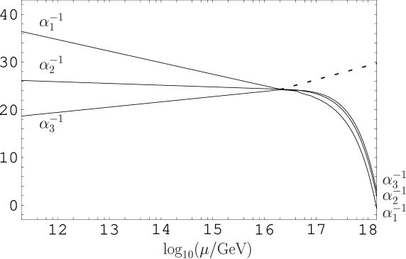
Figure 2: Energy dependence of gauge couplings. The input parameters are given by $\alpha^{-1}_{\textrm{\scriptsize em}}=127.906$, $\sin^{2}\theta_{w}=0.2312$ and $\alpha_{3}=0.1187$ at $M_{Z}=91.1876$GeV. $M_{\textrm{\scriptsize SUSY}}=M_{Z}$ and $1/(2R_{5})=2\times 10^{16}$GeV are chosen. The broken line indicates gauge couplings in minimal 4D supersymmetric grand unified model where $X,Y$ gauge bosons, two triplet Higgs fields and their superpartners in addition to standard model particles and superparticles lead to the coefficient of the $\beta$ function $b_{1}=b_{2}=b_{3}=-8$.

To evaluate energy dependence of gauge coupling constants, successful SU(5) relations are available. For zero mode, the gauge couplings $\alpha^{-1}_{\textrm{\scriptsize em}}=127.906$ and $\alpha_{s}=0.1187$ at $M_{Z}=91.1876\textrm{GeV}$ lead to the weak mixing angle

$$\sin^{2}\theta_{w}={5\over 5b_{1}+3b_{2}-8b_{3}}\left((b_{1}-b_{2}){\alpha_{\textrm{\scriptsize em}}\over\alpha_{s}}+(b_{2}-b_{3}){3\over 5}\right)=0.231,$$

which is compatible with experiments. As another version of zero mode renormalization group equations, the unified scale is written as

$$M_{X}=M_{Z}\,\textrm{exp}\left[{16\pi\over 5}{\alpha_{\textrm{\scriptsize em}}^{-1}(M_{Z})\over(b_{1}-b_{2})}\left({3\over 8}-\sin^{2}\theta_{w}(M_{Z})\right)\right]=1.99\times 10^{16}\textrm{GeV}.$$ (4.34)

In order to solve the doublet-triplet splitting by boundary conditions, we choose $1/(2R_{5})=M_{X}$. In Figure 4, $\alpha_{\textrm{\scriptsize em}}$, $\alpha_{3}$ and $\sin^{2}\theta_{w}$ at $M_{Z}$ are taken as input parameters and the radius is chosen as $1/(2R_{5})=2\times 10^{16}\textrm{GeV}$. The couplings $\alpha^{-1}$ approach to zero above $10^{18}\textrm{GeV}$. In order for this model with rapidly growing strong coupling at high energies to be valid, the scale $1/R_{6}$ has the upper bound.

4.3 Yukawa couplings

The values of the running quark masses $m(\mu)$ below the electroweak scale $\Lambda_{W}$ can be evaluated by using the formula $\mu(d/d\mu)m(\mu)=\gamma(\alpha_{s})m(\mu)$ where $\gamma(\alpha_{s})$ denotes the anomalous dimension of the quark mass operator. On the other hand, at high energies far from $\Lambda_{W}$, evolution equations of Yukawa coupling constants $y(\mu)$ are needed for the quark masses. With $1/(2R_{5})$ as the unification scale to solve the doublet-triplet splitting, we have seen that $1/R_{6}$ should be less than the scale where $\alpha^{-1}$ is zero. In this light, the values of the parameters $R_{5}$, $R_{6}$ and $g$ are almost fixed although a variation is still possible. It should be checked whether the values of derived Yukawa coupling constants are compatible with experiments and whether effects of extra dimensions are useful for generating hierarchical numbers.

We examine Yukawa coupling constants at $\mu=1/(2R_{5})=M_{X}$ where the unified gauge group is broken by boundary conditions. At energies $\Lambda_{W}\leq\mu\leq M_{X}$, renormalization group equations are governed by contributions of zero mode, but still with extra-dimensional effects as seen from the factors $(1/\sqrt{\pi R_{5}})$ and $(1/\sqrt{\pi R_{6}})$ in Table 5. For experimental data, we adopt the values of the running Yukawa coupling for quarks and charged leptons shown in Table 7 by quoting Ref.[21]. The values of quark and lepton masses are sensitive to the value of $\tan\beta=v_{2}/v_{1}$. We choose $\tan\beta=10$, avoiding too large or too small $\tan\beta$ which can give rise to the burst of Yukawa coupling constants. As the numerical results of Yukawa coupling constants are not sensitive to the value of $M_{\textrm{\scriptsize SUSY}}$, the scale of the supersymmetry breaking is taken as $M_{\textrm{\scriptsize SUSY}}=M_{Z}$.

Table 7: Yukawa coupling constants at $M_{Z}$ and $M_{X}$. For convenience, instead of the Yukawa coupling constants $y(\mu)$, the values of $m(\mu)=y(\mu)v\sin\beta/\sqrt{2}$ for up-type quarks and $m(\mu)=y(\mu)v\cos\beta/\sqrt{2}$ for down-type quarks and charged leptons are listed in unit of MeV, where $v=\sqrt{2}\Lambda_{W}$, $\Lambda_{W}=174.1$GeV, $\tan\beta=v_{2}/v_{1}=10$ and $M_{\textrm{\scriptsize SUSY}}=M_{Z}$.

$\mu$	$m_{u}(\mu)$	$m_{c}(\mu)$	$m_{t}(\mu)$	$m_{d}(\mu)$	$m_{s}(\mu)$	$m_{b}(\mu)$	$m_{e}(\mu)$	$m_{\mu}(\mu)$	$m_{\tau}(\mu)$
$M_{Z}$	2.33	677	181000	4.69	93.4	3000	0.4868	102.751	1746.7
$M_{X}$	1.04	302	129000	1.33	26.5	1000	0.3250	68.598	1171.4

The Yukawa couplings arise as superpotential terms of the fixed point coupling (2.54) where delta functions should be read as $\delta(x^{5})\delta(x^{6}-\pi R_{6})$. The up-type Yukawa superpotential $f_{u}$ is given by

$$f_{u}=\left(\begin{array}[]{c}T_{1}\\ T_{2}\\ T_{3}\\ \end{array}\right)^{\!\!\!T\,ij}\!\!\left(\begin{array}[]{ccccc}Y_{u11}^{\prime}&Y_{u12}^{\prime}&0&0&0\\ Y_{u21}^{\prime}&Y_{u22}^{\prime}&0&0&0\\ Y_{u31}^{\prime}&Y_{u32}^{\prime}&Y_{u31}&Y_{u32}&Y_{u33}\\ \end{array}\right)\!\!\left(\begin{array}[]{c}T_{1}^{\prime}\\ T_{2}^{\prime}\\ T_{1}\\ T_{2}\\ T_{3}\\ \end{array}\right)^{\!\!lm}\!\!\!H_{2}^{n}\epsilon_{ijlmn},$$ (4.46)

where $i,j,l,m,n=1,\cdots,5$. The Yukawa couplings are taken for boundary values of fields rather than they are for zero mode. In terms of the dimensionless Yukawa coupling constants $y_{u\jmath\imath}^{\prime}$ and $y_{u3\jmath}$ ($\jmath=1,2,3$, $\imath=1,2$) normalized with the cutoff of 6D theory $M_{s}$, the Yukawa coupling constant matrix is written as

$$\left(\begin{array}[]{ccccc}{1\over M_{s}^{3/2}}y_{u11}^{\prime}&{1\over M_{s}^{3/2}}y_{u12}^{\prime}&0&0&0\\ {1\over M_{s}^{3/2}}y_{u21}^{\prime}&{1\over M_{s}^{3/2}}y_{u22}^{\prime}&0&0&0\\ {1\over M_{s}}y_{u31}^{\prime}&{1\over M_{s}}y_{u32}^{\prime}&{1\over M_{s}}y_{u31}&{1\over M_{s}}y_{u32}&{1\over\sqrt{M_{s}}}y_{u33}\\ \end{array}\right).$$ (4.50)

When the Higgs field is replaced with the vacuum expectation value $\langle H_{2}^{2}\rangle=v_{2}/\sqrt{\pi R_{5}}$, the zero mode leads to the 4D up-type quark mass term at $\mu=M_{X}$ in the notation given in Table 5,

$$\left(\begin{array}[]{c}u_{1}\\ u_{2}\\ u_{3}\\ \end{array}\right)^{T}\left(\begin{array}[]{ccc}\epsilon_{5}^{3}\,y_{u11}^{\prime}v_{2}&\epsilon_{5}^{3}\,y_{u12}^{\prime}v_{2}&\epsilon_{5}^{2}\,y_{u31}v_{2}\\ \epsilon_{5}^{3}\,y_{u21}^{\prime}v_{2}&\epsilon_{5}^{3}\,y_{u22}^{\prime}v_{2}&\epsilon_{5}^{2}\,y_{u32}v_{2}\\ \epsilon_{5}^{2}\,y_{u31}^{\prime}v_{2}&\epsilon_{5}^{2}\,y_{u32}^{\prime}v_{2}&\epsilon_{5}\,y_{u33}v_{2}\\ \end{array}\right)\left(\begin{array}[]{c}u_{1}^{c}\\ u_{2}^{c}\\ u_{3}^{c}\\ \end{array}\right)+\textrm{H.c.},$$ (4.60)

where $\epsilon_{5}=1/\sqrt{\pi R_{5}M_{s}}$. The mass matrix in Eq.(4.60) in general has nonzero off-diagonal components in flavor space. It should be diagonalized into mass eigenstates. As an example to estimate the size of Yukawa couplings, we here compare diagonal components in Eq.(4.60) with the values shown in Table 7. For $1/(2R_{5})=2\times 10^{16}$GeV, $\tan\beta=10$ and $M_{s}=10^{18}$GeV, we obtain the Yukawa coupling constants as

$$y_{u11}^{\prime}\approx 0.003,\quad~{}y_{u22}^{\prime}\approx 0.9,\quad~{}y_{u33}\approx 2.$$ (4.61)

The mass hierarchy is generated as

$${m_{u}\over m_{t}}(=8.06\times 10^{-6}) \!\!\!\ll\!\!\! {y_{u11}^{\prime}\over y_{u33}}(\approx 0.0015),$$ (4.62)

$${m_{c}\over m_{t}}(=0.00234) \!\!\!\ll\!\!\! {y_{u22}^{\prime}\over y_{u33}}(\approx 0.45).$$ (4.63)

due to the suppression $\epsilon_{5}\approx 0.1$.

The down-type and charged-lepton-type Yukawa couplings are generated from the superpotential

$$f_{d} \!\!\!=\!\!\! \left(\begin{array}[]{c}T_{1}\\ T_{2}\\ T_{3}\\ \end{array}\right)^{\!\!\!T\,ij}\left(\begin{array}[]{ccc}{1\over M_{s}^{3/2}}\,y_{d11}&{1\over M_{s}^{3/2}}\,y_{d12}&{1\over M_{s}^{3/2}}\,y_{d13}\\ {1\over M_{s}^{3/2}}\,y_{d21}&{1\over M_{s}^{3/2}}\,y_{d22}&{1\over M_{s}^{3/2}}\,y_{d23}\\ {1\over M_{s}}\,y_{d31}&{1\over M_{s}}\,y_{d32}&{1\over M_{s}}\,y_{d33}\\ \end{array}\right)\left(\begin{array}[]{c}\Psi_{1}\\ \Psi_{2}\\ \Psi_{3}\\ \end{array}\right)_{\!\!i}H_{1\,j}$$ (4.81)

$$+\left(\begin{array}[]{c}T_{1}^{\prime}\\ T_{2}^{\prime}\\ \end{array}\right)^{\!\!T\,ij}\left(\begin{array}[]{ccc}{1\over M_{s}^{3/2}}\,y_{e11}&{1\over M_{s}^{3/2}}\,y_{e12}&{1\over M_{s}^{3/2}}\,y_{e13}\\ {1\over M_{s}^{3/2}}\,y_{e21}&{1\over M_{s}^{3/2}}\,y_{e22}&{1\over M_{s}^{3/2}}\,y_{e23}\\ \end{array}\right)\left(\begin{array}[]{c}\Psi_{1}\\ \Psi_{2}\\ \Psi_{3}\\ \end{array}\right)_{\!\!i}H_{1\,j},$$

where the Yukawa coupling constants $y_{d\imath\jmath}$, $y_{d3\jmath}$ and $y_{e\imath\jmath}$ ($\jmath=1,2,3$, $\imath=1,2$) are normalized to be dimensionless with the cutoff of 6D theory $M_{s}$. From this equation, with the vacuum expectation value $\langle H_{1,\,j=2}\rangle=v_{1}/\sqrt{\pi R_{5}}$ and the notation of zero-mode given in Table 5, the 4D down-type quark and charged lepton mass terms are

$$\left(\begin{array}[]{c}d_{1}\\ d_{2}\\ d_{3}\\ \end{array}\right)^{T}\left(\begin{array}[]{ccc}\epsilon_{5}^{2}\epsilon_{6}\,y_{d11}v_{1}&\epsilon_{5}^{2}\epsilon_{6}\,y_{d12}v_{1}&\epsilon_{5}^{2}\epsilon_{6}\,y_{d13}v_{1}\\ \epsilon_{5}^{2}\epsilon_{6}\,y_{d21}v_{1}&\epsilon_{5}^{2}\epsilon_{6}\,y_{d22}v_{1}&\epsilon_{5}^{2}\epsilon_{6}\,y_{d23}v_{1}\\ \epsilon_{5}\epsilon_{6}\,y_{d31}v_{1}&\epsilon_{5}\epsilon_{6}\,y_{d32}v_{1}&\epsilon_{5}\epsilon_{6}\,y_{d33}v_{1}\\ \end{array}\right)\left(\begin{array}[]{c}d_{1}^{c}\\ d_{2}^{c}\\ d_{3}^{c}\\ \end{array}\right)$$ (4.91)

$$+\left(\begin{array}[]{c}e_{1}^{c}\\ e_{2}^{c}\\ e_{3}^{c}\\ \end{array}\right)^{T}\left(\begin{array}[]{ccc}\epsilon_{5}^{2}\epsilon_{6}\,y_{e11}v_{1}&\epsilon_{5}^{2}\epsilon_{6}\,y_{e12}v_{1}&\epsilon_{5}^{2}\epsilon_{6}\,y_{e13}v_{1}\\ \epsilon_{5}^{2}\epsilon_{6}\,y_{e21}v_{1}&\epsilon_{5}^{2}\epsilon_{6}\,y_{e22}v_{1}&\epsilon_{5}^{2}\epsilon_{6}\,y_{e23}v_{1}\\ \epsilon_{5}\epsilon_{6}\,y_{d31}v_{1}&\epsilon_{5}\epsilon_{6}\,y_{d32}v_{1}&\epsilon_{5}\epsilon_{6}\,y_{d33}v_{1}\\ \end{array}\right)\left(\begin{array}[]{c}e_{1}\\ e_{2}\\ e_{3}\\ \end{array}\right)+\textrm{H.c.},$$ (4.101)

where $\epsilon_{6}=1/\sqrt{\pi R_{6}M_{s}}(>\epsilon_{5})$. The down-type quarks and charged leptons have the common Yukawa coupling constants in $\sum_{\jmath=1}^{3}y_{d3\jmath}(d_{3}d_{\jmath}^{c}+e_{3}^{c}e_{\jmath})+\textrm{H.c.}$. Because the two matrices for down-type quarks and charged leptons are distinct, the fermion mass relations are avoided. The relation between $m_{b}$ and $m_{\tau}$ also depends on the form of the matrices. The difference of $m_{b}$ and $m_{\tau}$ in data might yield as a result of diagonalization of the matrices with the common and uncommon components. As an example of estimation, we compare diagonal components in Eq.(4.101) with data at $M_{X}$ in Table 7. For $R_{6}=R_{5}/10$, we obtain the Yukawa coupling constants as

$$y_{d11}\approx 0.01,\quad~{}y_{d22}\approx 0.2,\quad~{}y_{d33}\approx 0.1,\quad~{}y_{e11}\approx 0.003,\quad~{}y_{e22}\approx 0.6.$$ (4.102)

The mass hierarchy is generated as

$${m_{d}\over m_{b}}(=0.00133) \!\!\!\ll\!\!\! {y_{d11}\over y_{d33}}(\approx 0.1),$$ (4.103)

$${m_{s}\over m_{b}}(=0.0265) \!\!\!\ll\!\!\! {y_{d22}\over y_{d33}}(\approx 2),$$ (4.104)

$${m_{e}\over m_{\tau}}(=2.774\times 10^{-4}) \!\!\!\ll\!\!\! {y_{e11}\over y_{d33}}(\approx 0.03),$$ (4.105)

$${m_{\mu}\over m_{\tau}}(=0.0585) \!\!\!\ll\!\!\! {y_{e22}\over y_{d33}}(\approx 6),$$ (4.106)

due to the suppression $\epsilon_{5}\approx 0.1$ and $\epsilon_{6}\approx 0.3$. We have chosen $\tan\beta=10$. For such a moderate value, the suppression factor $\epsilon_{6}$ provides a part of the suppression for $m_{b}/m_{t}$. The effect of $v_{2}>v_{1}$ is partly compensated by the effect of $R_{6}<R_{5}$. The mass matrices could also be compared with data taking into account the Cabibbo-Kobayashi-Maskawa matrix. For example, in the base where up-type quarks are diagonal, the down-type quark mass matrix may be [21] (as each component is written in absolute value)

$$M_{d}(M_{X})=m_{b}(M_{X})\left(\begin{array}[]{ccc}0.0026&0.0054&0.0025\\ 0.0054&0.0263&0.0310\\ 0.0025&0.0310&0.9990\\ \end{array}\right).$$ (4.110)

Then the corresponding Yukawa matrix is written as

$$\left(\begin{array}[]{ccc}y_{d11}&y_{d12}&y_{d13}\\ y_{d21}&y_{d22}&y_{d23}\\ y_{d31}&y_{d32}&y_{d33}\\ \end{array}\right)\approx y_{d33}\left(\begin{array}[]{ccc}0.1&0.1&0.1\\ 0.1&1&1\\ 0.001&0.01&1\\ \end{array}\right)$$ (4.117)

Similarly to estimation from diagonal components of mass matrices, small numbers are generated via the suppression factor $\epsilon_{5}$ and $\epsilon_{6}$.

4.4 Proton stability

As in the 4D minimal SU(5) unified model, extra fields which become dynamical at $\mu=1/(2R_{5})=M_{X}$ can give rise to baryon number violating processes. Contributions of $X$, $Y$ gauge boson exchange give dimension-six baryon-number violating operators. Their amplitudes are suppressed by $M_{X}$ which is large in supersymmetric case. As supersymmetric contributions, dimension-four and dimension-five proton decay operators can yield unless some selection rules are applied.

For the field content given in Table 5, the superfields $T^{ij}$, $\Psi_{\imath}$, $H_{1i}$, $H_{1}^{ci}$, $H_{2}^{i}$ and $H_{2i}^{c}$ ($i,j=1,\cdots,5$) give the gauge-singlet lower dimension operators on the fixed point like the Yukawa couplings,

$$\Psi_{\imath}H_{2}^{i},~{}~{}\Psi_{\imath}H_{1}^{c\,i},~{}~{}H_{2}^{i}H_{1i},~{}~{}H_{2}^{i}H_{2i}^{c},~{}~{}H_{1i}H_{1}^{c\,i},~{}~{}H_{2i}^{c}H_{1}^{c\,i},~{}~{}T^{ij}H_{1i}H_{2j}^{c},$$ (4.118)

$$T^{ij}\Psi_{\imath}H_{1j},\quad~{}T^{ij}T^{kl}H_{2}^{m}\varepsilon_{ijklm},$$ (4.119)

$$T^{ij}\Psi_{\imath}H_{2j}^{c},\quad~{}T^{ij}T^{kl}H_{1}^{c\,m}\varepsilon_{ijklm}$$ (4.120)

$$T^{ij}T^{kl}T^{mn}\Psi_{n}\varepsilon_{ijklm},~{}~{}T^{ij}T^{kl}T^{mn}H_{1n}\varepsilon_{ijklm},~{}~{}T^{ij}T^{kl}T^{mn}H_{2n}^{c}\varepsilon_{ijklm},$$ (4.121)

where $T^{ij}$ collectively denotes $T_{\imath}^{ij}$, $T_{\imath}^{\prime}{}^{ij}$ and $T_{3}^{ij}$ ($\imath=1,2$) and for $\Psi$, $\bf{5}^{*}$-part $\Psi_{\jmath i}$ ($\jmath=1,2,3$) is coupled to other fields. The operators (4.119) gives the Yukawa couplings as shown in Eqs.(4.46) and (4.81). If the operators (4.120) exist, they would give dimension-five baryon number violation processes by colored higgsino exchange. If $\Psi_{\imath}H_{2}^{i}$ and $H_{2}^{i}H_{1i}$ exist, they would generate large masses for the weak-doublet Higgs fields, which gives rise to recurrence of the doublet-triplet splitting problem. These dangerous operators are avoided by R invariance as a subgroup of SU(2)${}_{\textrm{\scriptsize R}}$ inherent in 6D $N=2$ theory. In Table 8, R charges of superfields are shown.

Table 8: R-charges in 5D Higgs model.

$\theta$	$V$, $\Sigma_{5}$, $\Sigma_{6}$	$\Phi$	$H_{1}$, $H_{2}$	$H_{1}^{c}$, $H_{2}^{c}$	$T$, $\Psi$, $N$	$S$	$X$	$B$	$\bar{B}$
$-1$	0	2	0	2	1	0	2	2	$-2$

With this charge assignment, the 5D mass operators $H_{2}H_{2}^{c}$ and $H_{1}H_{1}^{c}$ as well as the Yukawa couplings $T\Psi H_{1}$ and $TTH_{2}$ are only allowed in Eqs.(4.118)-(4.121). While R invariance prohibits operators of dimension four and five, $T\Psi H_{1}$ and $TTH_{2}$ give dimension-six baryon number violation processes by colored Higgs exchange. The diagrams for these dimension-six operators are shown in Fig. 3,

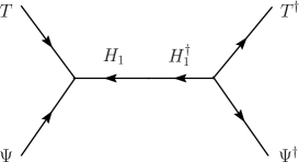
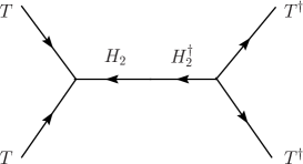
Figure 3: Dimension-six baryon number violating process.

where two groups of superfields of different chirality are connected by a chirality non-flip superpropagator. The lifetime is proportional to $\tau\propto(1/(2R_{5}))^{4}$, which for $1/(2R_{5})=M_{X}$ is compatible with the observation.

4.5 Supersymmetry breaking

So far we have worked with the supersymmetries $N=2$ in 6D bulk (4D $N=4$), $N=1$ on 5D fixed lines (4D $N=2$) and $N=1$ on 4D fixed points (4D $N=1$). In this section, we consider breaking 4D $N=1$ supersymmetry to no supersymmetry.

The supersymmetry breaking term is effectively generated on the 4D fixed point where the gauge multiplet is directly coupled,

$$\int d^{6}x\,\delta(x^{5}-\pi R_{5})\delta(x^{6})\,2\textrm{Re}\left[\textrm{Tr}{1\over 4kg^{2}}SW^{\alpha}W_{\alpha}\right]_{F}.$$ (4.122)

From the configuration shown in Table 4, the superfield $S$ is spatially separated from all fields except for the 6D gauge multiplet ($V,\Sigma_{5},\Sigma_{6},\Phi$). The 6D fields $\Sigma_{5}$, $\Sigma_{6}$ and $\Phi$ do not have zero mode. As long as leading zero mode part of supersymmetry breaking effect is concerned, the model is similar to the model of Ref.[12] where the standard-model gauge fields and gauginos only propagate in bulk. At $\mu=M_{X}$ gauginos obtain masses through their direct couplings (4.122) as

$$2\textrm{Re}\left[{1\over M_{s}}SW^{\alpha}W_{\alpha}\right]_{F}\supset M_{1/2}\lambda^{\alpha}\lambda_{\alpha},\qquad~{}M_{1/2}={F_{S}\over M_{s}}$$ (4.123)

via $S=F_{S}\theta\theta$. All other supersymmetry breaking masses are suppressed by a Yukawa factor of the spatial separation of the source and matter and by loop factors $\alpha^{2}$. Their masses are generated via running. For squarks, sleptons and higgsino whose masses are denoted as $\tilde{m}$ collectively, one-loop renormalization group equations have the form [22][23][24]

$${d\tilde{m}^{2}\over dt}=-c_{g}g^{2}M_{1/2}^{2}+c_{m}g^{2}\textrm{Tr}Y\tilde{m}^{2}+c_{y}y^{2}m_{\tilde{h}}^{2},$$ (4.124)

where $c_{g}$ and $c_{y}$ are positive coefficients and $c_{m}$ are not necessarily positive and the higgsino mass is denoted as $m_{\tilde{h}}$. The renormalization group flow starts to grow with the gaugino contribution with a negative sign in the direction of low energies from the unification scale. This do not lead to new flavor violation because the sources of flavor violation are aligned with the Yukawa matrices. At one loop approximation, gaugino masses are proportional to gauge couplings squared

$${M_{1}\over\alpha_{1}}={M_{2}\over\alpha_{2}}={M_{3}\over\alpha_{3}}={M_{1/2}\over\alpha_{X}}.$$ (4.125)

Since $\alpha_{1}$, $\alpha_{2}$, $\alpha_{3}$ and $\alpha_{X}$ are of the same order, the gaugino masses $M_{1}$, $M_{2}$, $M_{3}$ and $M_{1/2}$ are of the same order. That charged superparticles and the lightest Higgs have lower bounds gives the minimum of gaugino mass at the unification scale. For $M_{1/2}=350\textrm{GeV}$ ($M_{1}=144\textrm{GeV}$, $M_{2}=287\textrm{GeV}$, $M_{3}=1009\textrm{GeV}$) and $M_{s}=10^{18}\textrm{GeV}$, $\sqrt{F_{S}}=5.9\times 10^{10}\textrm{GeV}$. Since $F_{S}$ is generated at $\mu=M_{s}$, it would be natural that $F_{S}\sim M_{s}$. In order to produce a small $F_{S}$, one may apply a mechanism in Ref.[25][26] by utilizing the two extra dimensions. Following this idea, it may also be possible to address naturalness for $\mu$-term by setting fields confined on fixed lines. Here we do not treat this issue further.

All soft supersymmetry breaking masses are of the same order at the electroweak scale. It is possible that neutralino or slepton has the mass $\lesssim 200$ GeV. The lightest superparticle (LSP) can be gravitino $m_{3/2}\sim F_{S}/M_{Pl}$ with the Planck scale $M_{Pl}$ as in case of Ref.[24]. Like models given in Refs.[12][13], the number of input parameters might be taken as four where $\tan\beta$ is treated as a free parameter.fixed value of tan$\beta=10$, The quantity tan $\beta$ affects the third generation in running. Charged lepton mass matrix includes $\tan\beta$ in off diagonal components. If tan$\beta$ is increased, it means a large mixing. Consequently stau mass is decreased. For a large tan$\beta$, an input $M_{1/2}$ must be large in order not to make stau too light. Further consideration about these issues and high energy behavior of gauge couplings would restrict the model.

Before concluding the model with Higgs fields as 5D superfields, we mention other choice of parity matrices. Similar results are also obtained for another choice of parity matrices

$$P_{1}=P_{3}={\bf 1}_{6},\quad~{}P_{2}=\left(\begin{array}[]{cc}{\bf 1}_{3}&\\ &-{\bf 1}_{3}\\ \end{array}\right),\quad~{}P_{4}=\left(\begin{array}[]{ccccc|c}{\bf 1}_{5}&\\ &-1\\ \end{array}\right).$$ (4.130)

The difference between Eq.(4.130) and Eq.(4.5) is the numbers of the components $V^{(--+-)}$, $\Sigma_{5}^{(+++-)}$, $\Sigma_{6}^{(---+)}$, $\Phi^{(++-+)}$ and $V^{(-++-)}$, $\Sigma_{5}^{(+-+-)}$, $\Sigma_{6}^{(-+-+)}$, $\Phi^{(+--+)}$. These affect dynamics at scales beyond $1/(2R_{6})$. The boundary conditions for Eq.(4.130) are shown in Appendix (C.2).

5 Model with Higgs in gauge multiplet

From here on we consider a model where Higgs fields are components of the 6D gauge multiplets, which is a 6D version of the model given in [9]. The parity matrices are given by

$$P_{1}=\left(\begin{array}[]{cc}{\bf 1}_{5}&\\ &-1\\ \end{array}\right),\quad~{}P_{2}=\left(\begin{array}[]{cc}{\bf 1}_{2}&\\ &-{\bf 1}_{4}\\ \end{array}\right),\quad~{}P_{3}=P_{4}={\bf 1}_{6},$$ (5.5)

for the equations (LABEL:parityg5) and (LABEL:parityg6). The vector superfield $V(A^{m},\lambda)$ has the boundary conditions

$$\left(\begin{array}[]{cc|ccc|c}_{(++++)}&{}_{(++++)}&{}_{(+-++)}&{}_{(+-++)}&{}_{(+-++)}&{}_{(--++)}\\ _{(++++)}&{}_{(++++)}&{}_{(+-++)}&{}_{(+-++)}&{}_{(+-++)}&{}_{(--++)}\\ \hline\cr_{(+-++)}&{}_{(+-++)}&{}_{(++++)}&{}_{(++++)}&{}_{(++++)}&{}_{(-+++)}\\ _{(+-++)}&{}_{(+-++)}&{}_{(++++)}&{}_{(++++)}&{}_{(++++)}&{}_{(-+++)}\\ _{(+-++)}&{}_{(+-++)}&{}_{(++++)}&{}_{(++++)}&{}_{(++++)}&{}_{(-+++)}\\ \hline\cr_{(--++)}&{}_{(--++)}&{}_{(-+++)}&{}_{(-+++)}&{}_{(-+++)}&{}_{(++++)}\\ \end{array}\right).$$ (5.12)

Similarly to the model with 5D Higgs in Section 4, the zero mode $(++++)$ is in the blocks of square matrices of rank 2, 3 and 1. They have the unbroken gauge group SU(3)${}_{\textrm{\scriptsize C}}$$\times$SU(2)${}_{\textrm{\scriptsize W}}$$\times$U(1)_Y$\times$U(1)^′. The U(1)${}_{\textrm{\scriptsize em}}$ and U(1)^′ charge matrices are given by Eqs.(4.14) and (4.15), respectively. As in the previous section, this gives the correct normalization for hypercharges. The SU(5) relation for MSSM gauge coupling constants is maintained. The difference from the case with 5D Higgs is that the the boundary conditions $(--++)$ and $(-+++)$ appear. The whole block has all the positive parity in the $x^{6}$ direction. They becomes dynamical when the extra dimension $x^{5}$ is visible. For each fixed line and point, unbroken gauge groups of restricted gauge symmetry and the number of supersymmetry in the language of 4D are tabulated in Table 9.

Table 9: Gauge groups and supersymmetries $N$ on fixed lines and points.

Location	Gauge group	$N$	Location	Gauge group	$N$
$x^{6}=0$	SU(6)	2	$(0,0)$	SU(5)$\times$U(1)′	1
$x^{6}=\pi R_{6}$	SU(6)	2	$(0,\pi R_{6})$	SU(5)$\times$U(1)′	1
$x^{5}=0$	SU(5)$\times$U(1)′	2	$(\pi R_{5},0)$	SU(4)$\times$SU(2)$\times$U(1)	1
$x^{5}=\pi R_{5}$	SU(4)$\times$SU(2)$\times$U(1)	2	$(\pi R_{5},\pi R_{6})$	SU(4)$\times$SU(2)$\times$U(1)	1

In the gauge multiplet, the superfield $\Sigma_{5}(\sigma_{5},\lambda_{5})$ has the boundary condition,

$$\left(\begin{array}[]{cc|ccc|c}_{(--++)}&{}_{(--++)}&{}_{(-+++)}&{}_{(-+++)}&{}_{(-+++)}&{}_{(++++)}\\ _{(--++)}&{}_{(--++)}&{}_{(-+++)}&{}_{(-+++)}&{}_{(-+++)}&{}_{(++++)}\\ \hline\cr_{(-+++)}&{}_{(-+++)}&{}_{(--++)}&{}_{(--++)}&{}_{(--++)}&{}_{(+-++)}\\ _{(-+++)}&{}_{(-+++)}&{}_{(--++)}&{}_{(--++)}&{}_{(--++)}&{}_{(+-++)}\\ _{(-+++)}&{}_{(-+++)}&{}_{(--++)}&{}_{(--++)}&{}_{(--++)}&{}_{(+-++)}\\ \hline\cr_{(++++)}&{}_{(++++)}&{}_{(+-++)}&{}_{(+-++)}&{}_{(+-++)}&{}_{(--++)}\\ \end{array}\right).$$ (5.19)

The superfield $\Sigma_{5}$ has two SU(2) doublet as zero mode. These zero modes are identified as the two MSSM Higgs fields. In addition, the whole block of $\Sigma_{5}$ also has the positive parity in the $x^{6}$ direction. They becomes dynamical when the extra dimension $x^{5}$ is visible. The superfields $\Sigma_{6}$ and $\Phi$ have the negative parity in the $x^{6}$ direction. They are non-dynamical up to the scale $1/(2R_{6})$. The boundary conditions for $\Sigma_{6}$ and $\Phi$ are given in Appendix C.2.

We take confined fields on a fixed line as matter. The field content is shown in Table 10 with a consideration similar to that in obtaining explicit boundary conditions given in Table 2.

Table 10: Field content added to the gauge multiplet $(V,\Sigma_{5},\Sigma_{6},\Phi)(x,x^{5},x^{6})$ in the model with Higgs fields in the gauge multiplet. Quantum numbers are shown for gauge groups of the restricted gauge symmetry on each fixed line or point. Here $\jmath=1,2,3$.

Location	Field	Quantum number		$\eta_{1}$	$\eta_{2}$
$x^{6}=\pi R_{6}$	$(N_{\jmath},N_{\jmath}^{c})(x,x^{5})$	6	$\in$ SU(6)	$-1$	$1$
	$(E_{\jmath},E_{\jmath}^{c})(x,x^{5})$	15		1	1
	$(D_{\jmath},D_{\jmath}^{c})(x,x^{5})$	15∗		$-1$	1
	$(U_{\jmath},U_{\jmath}^{c})(x,x^{5})$	20		1	$-1$
$(\pi R_{5},0)$	$S(x)$	$(1,1,0)$	$\in$ SU(4)$\times$SU(2)$\times$U(1)	—

Quantum numbers are shown for charge-unconjugated. For all fields on the fixed line (not $S$ on a fixed point), negative 5D masses $M<0$ are chosen so that $N_{\jmath}$, $E_{\jmath}$, $D_{\jmath}$ and $U_{\jmath}$ are localized at $x^{5}=\pi R_{5}$. The decoupling of redundant components will be taken into account so that zero mode field content is the same as the model of 5D Higgs with the identical unbroken gauge group. It is 4D gauge anomaly free.

Gauge symmetry breaking of U(1)^′ is simultaneously treated with the decoupling of redundant components of fields in next section.

5.1 Mass spectrum

In this section, following [9] we start with reviewing that the fields given in Table 10 include redundant components, that it can decouple with fixed-line interactions described in Section 2.4 and that this decoupling is responsible for flavor mixing. After this decoupling is performed, we give quantum numbers for components of zero mode and KK modes of the 6D gauge multiplet and the fields given in Table 10.

The boundary conditions for the matter superfields are given by

$$N_{\jmath} \!\!\!=\!\!\! \left[N_{\bar{l}^{\prime}}^{(--)}\right]{}_{\jmath}\oplus\left[N_{\bar{d}^{\prime}}^{(-+)}\oplus N_{n}^{(++)}\right]{}_{\jmath},$$ (5.20)

$$E_{\jmath} \!\!\!=\!\!\! \left[E_{e}^{(++)}\right]{}_{\jmath}\oplus\left[E_{u}^{(++)}\oplus E_{\bar{d}}^{(-+)}\right]{}_{\jmath}\oplus\left[E_{q}^{(+-)}\oplus E_{\bar{l}}^{(--)}\right]{}_{\jmath},$$ (5.21)

$$D_{\jmath} \!\!\!=\!\!\! \left[D_{\bar{e}}^{(-+)}\right]{}_{\jmath}\oplus\left[D_{\bar{u}}^{(-+)}\oplus D_{d}^{(++)}\right]{}_{\jmath}\oplus\left[D_{\bar{q}}^{(--)}\oplus D_{l}^{(+-)}\right]{}_{\jmath},$$ (5.22)

$$U_{\jmath} \!\!\!=\!\!\! \left[U_{u^{\prime}}^{(++)}\oplus U_{\bar{e}^{\prime}}^{(-+)}\right]{}_{\jmath}\oplus\left[U_{e^{\prime}}^{(++)}\oplus U_{\bar{u}^{\prime}}^{(-+)}\right]{}_{\jmath}\oplus\left[U_{q^{\prime}}^{(+-)}+U_{\bar{q}^{\prime}}^{(--)}\right]_{\jmath},$$ (5.23)

In Table 10, the parities of sign have been chosen so that $N_{\jmath}$, $E_{\jmath}$, $D_{\jmath}$ and $U_{\jmath}$ have the $(++)$ components $N_{n\,\jmath}^{(++)}$, $E_{e\,\jmath}^{(++)}$, $D_{d\,\jmath}^{(++)}$ and $U_{u^{\prime}\,\jmath}^{(++)}$. Here the subscript Roman indices label SU(3)_C $\times$ SU(2)_W $\times$ U(1)_Y $\times$ U(1)^′ quantum numbers shown in Table 11. The quantum numbers are represented for for left-handed superfields.

Table 11: Quantum numbers and labels.

$q$ $(3,2,1/6,6p)$	$q^{\prime}$ $(3,2,1/6,-9p)$	$l$ $(1,2,-1/2,12p)$	$l^{\prime}$ $(1,2,-1/2,-3p)$
$u$ $(3^{*},1,-2/3,6p)$	$u^{\prime}$ $(3^{*},1,-2/3,-9p)$	$e$ $(1,1,1,6p)$	$e^{\prime}$ $(1,1,1,-9p)$
$d$ $(3^{*},1,1/3,12p)$	$d^{\prime}$ $(3^{*},1,1/3,-3p)$	$n$ $(1,1,0,-15p)$

The labels with a bar over a symbol are used to indicate each opposite quantum number such as $\bar{q}$ for $(3^{*},2,-1/6,-6p)$. In Eqs.(5.20)–(5.23), the square brackets stand for the classification of multiplets under SU(4)$\times$SU(2)$\times$U(1), the unbroken gauge group at $x^{5}=\pi R_{5}$ where $N_{\jmath}$, $E_{\jmath}$, $D_{\jmath}$ and $U_{\jmath}$ are localized. The charge-conjugated fields are decomposed as

$$N^{c}_{\jmath} \!\!\!=\!\!\! \left[N_{l^{\prime}}^{c(++)}\oplus N_{d^{\prime}}^{c(+-)}\right]{}_{\jmath}\oplus\left[N_{\bar{n}}^{c(--)}\right]{}_{\jmath},$$ (5.24)

$$E^{c}_{\jmath} \!\!\!=\!\!\! \left[E_{\bar{e}}^{c(--)}\oplus E_{\bar{u}}^{c(--)}\oplus E_{\bar{q}}^{c(-+)}\right]{}_{\jmath}\oplus\left[E_{l}^{c(++)}\oplus E_{d}^{c(+-)}\right]{}_{\jmath},$$ (5.25)

$$D^{c}_{\jmath} \!\!\!=\!\!\! \left[D_{e}^{c(+-)}\oplus D_{u}^{c(+-)}\oplus D_{q}^{c(++)}\right]{}_{\jmath}\oplus\left[D_{\bar{l}}^{c(-+)}\oplus D_{\bar{d}}^{c(--)}\right]{}_{\jmath},$$ (5.26)

$$U^{c}_{\jmath} \!\!\!=\!\!\! \left[U_{\bar{u}^{\prime}}^{c(--)}\oplus U_{\bar{e}^{\prime}}^{c(--)}\oplus U_{\bar{q}^{\prime}}^{c(-+)}\right]{}_{\jmath}\oplus\left[U_{e^{\prime}}^{c(+-)}\oplus U_{u^{\prime}}^{c(+-)}\oplus U_{q^{\prime}}^{c(++)}\right]{}_{\jmath},$$ (5.27)

where square brackets denote the classification of multiplets under SU(5)$\times$U(1)^′, the unbroken gauge group at $x^{5}=0$ where $N_{\jmath}^{c}$, $E_{\jmath}^{c}$, $D_{\jmath}^{c}$ and $U_{\jmath}^{c}$ are localized.

The parity $(++)$ components are

$$(3,2,\textrm{${1\over 6}$}) D_{q\,\jmath}^{c\,(++)},U_{q^{\prime}\,\jmath}^{c\,(++)}\quad~{}(1,2,-\textrm{${1\over 2}$})~{}~{}N_{l^{\prime}\,\jmath}^{c\,(++)},E_{l\,\jmath}^{c\,(++)}$$ (5.28)

$$(3^{*},1,\textrm{${1\over 3}$}) D_{d\,\jmath}^{(++)}\quad\qquad\qquad~{}(1,1,0)\quad~{}N_{n\,\jmath}^{(++)}$$ (5.29)

$$(3^{*},1,-\textrm{${2\over 3}$}) U_{u^{\prime}\,\jmath}^{(++)},E_{u\,\jmath}^{(++)}\qquad~{}(1,1,1)\quad~{}E_{e\,\jmath}^{(++)},U_{e^{\prime}\,\jmath}^{(++)}$$ (5.30)

The three numbers in the parentheses denote the quantum numbers for SU(3)${}_{\textrm{\scriptsize C}}$, SU(2)${}_{\textrm{\scriptsize W}}$ and U(1)_Y in order. For all of 5D superfields, negative 5D masses $M<0$ have been chosen so that $N,E,D,U$ are localized at $x^{5}=\pi R_{5}$. Redundant components as massless modes are decoupled with fixed-point couplings shown in Section 2.4. The SU(2)-singlet superfields [$E_{\bar{d}}^{(-+)}\oplus E_{u}^{(++)}$] and [$U_{\bar{u}^{\prime}}^{(-+)}\oplus U_{e^{\prime}}^{(++)}$] are made heavy through their couplings to additional matters of $(6,1)$ and $(4^{*},1)$, respectively (in SU(4) $6^{*}=6$). The other fields localized at $x^{5}=0$ include SU(2) doublet (++) components. They are made heavy for linear combinations. This linear combination makes mixing between generations, while the original Yukawa couplings are diagonal in flavor space since Higgs fields are part of the gauge multiplet.

Now we specify part of SU(2) doublet. For quark sector, [$D_{q}^{c(++)}\oplus D_{d}^{c(+-)}\oplus D_{e}^{c(+-)}$]${}_{\jmath}\equiv D_{T\,\jmath}^{c}$ and [$U_{q^{\prime}}^{c(++)}\oplus U_{u^{\prime}}^{c(+-)}\oplus U_{e^{\prime}}^{c(+-)}$]${}_{\jmath}\equiv U_{T^{\prime}\,\jmath}^{c}$ have the quantum number $(10,6p)$ and $(10,9p)$ for SU(5)$\times$U(1)^′, respectively. The fixed-point couplings with U(1)^′ symmetry breaking are chosen as

$$\delta(x^{5})\delta(x^{6}-\pi R_{6})\bigg{(}[(U_{T^{\prime}\,\imath}^{c}\mathbf{M}_{1\imath\jmath}+D_{T\,\imath}^{c}\mathbf{M}_{2\imath\jmath}\bar{\cal B})\bar{T}_{\jmath}+{\cal X}({\cal B}\bar{\cal B}-\Lambda_{x}^{2})]_{\theta\theta}+\textrm{H.c.}\bigg{)}.$$ (5.31)

with the 4D Kähler terms. For the fixed-point fields, the quantum numbers with respect to SU(5)$\times$U(1)^′ are given by

$$\bar{T}_{\imath}~{}(10^{*},9p),\quad~{}{\cal B}~{}(1,15p),\quad~{}\bar{\cal B}~{}(1,-15p),\quad~{}{\cal X}~{}(1,0)$$ (5.32)

and $\mathbf{M}_{1\imath\jmath}$, $\mathbf{M}_{2\imath\jmath}$ and $\Lambda_{x}$ are constants. From the equation of motion for ${\cal X}$, the vacuum expectation values are developed

$$\langle{\cal B}\rangle=\langle\hat{\cal B}\rangle=\Lambda_{x}.$$ (5.33)

This breaks U(1)^′ gauge symmetry. After the U(1)^′ symmetry breaking, linear combinations with mixing between generations yields. The elements of the linear combinations are $U_{T^{\prime}1}^{c}$, $U_{T^{\prime}2}^{c}$, $U_{T^{\prime}3}^{c}$, $D_{T1}^{c}$, $D_{T2}^{c}$ and $D_{T3}^{c}$. These fields $U_{T^{\prime}\,\jmath}^{c}$ and $D_{T\,\jmath}^{c}$ are transformed into another basis $H_{T\,\jmath}$ and $T_{\jmath}$, where $H_{T\,\jmath}$ would be made heavy and $T_{\jmath}$ has quark doublet as its $(++)$ component. The transformation between the two basis is given by

$$U_{T^{\prime}}^{c}=H_{T}U_{1}+TU_{3},\quad~{}D_{T}^{c}=H_{T}U_{2}+TU_{4}.$$ (5.34)

Here the $3\times 3$ unitary matrices $U_{\ell}$, $\ell=1,\cdots,4$ are written as components of the $6\times 6$ unitary matrix

$$U=\left(\begin{array}[]{cc}U_{1}&U_{2}\\ U_{3}&U_{4}\\ \end{array}\right),$$ (5.37)

which mixes the 6 elements. Due to linear combinations with complex numbers, CP phases are included. After U(1)^′ is broken, relevant part of the fixed-point coupling (5.31) becomes

$$(U_{T^{\prime}}^{c},D_{T}^{c})\left(\begin{array}[]{c}\mathbf{M}_{1}\\ \mathbf{M}_{2}\Lambda_{x}\\ \end{array}\right)\bar{T}=(H_{T},T)\left(\begin{array}[]{c}U_{1}\mathbf{M}_{1}+U_{2}\mathbf{M}_{2}\Lambda_{x}\\ U_{3}\mathbf{M}_{1}+U_{4}\mathbf{M}_{2}\Lambda_{x}\\ \end{array}\right)\bar{T}.$$ (5.42)

For the non-heavy part $U_{3}\mathbf{M}_{1}+U_{4}\mathbf{M}_{2}\Lambda_{x}=0$, the matrix $\mathbf{M}_{2}$ is written in terms of other variables as $\mathbf{M}_{2}=-\Lambda_{x}^{-1}U_{4}^{-1}U_{3}\mathbf{M}_{1}$. Eq.(5.42) reduces to

$$(U_{T^{\prime}}^{c}\mathbf{M}_{1}+D_{T}^{c}\mathbf{M}_{2}\Lambda_{x})\bar{T}=H_{T}(U_{1}-U_{2}U_{4}^{-1}U_{3})\mathbf{M}_{1}\bar{U}^{\dagger}(\bar{U}\bar{T}).$$ (5.43)

We choose $U$, $\mathbf{M}_{1}$ and $\bar{U}$ so that $(U_{1}-U_{2}U_{4}^{-1}U_{3})\mathbf{M}_{1}\bar{U}^{\dagger}$ is diagonal and the diagonal components are large. Thus $H_{T}$ becomes non-dynamical. From Eq.(5.42), zero mode is obtained as

$$U_{q^{\prime}}^{c(++)}=q(x)g_{0U}^{(++)}U_{3},\quad~{}D_{q}^{c(++)}=q(x)g_{0D}^{(++)}U_{4},$$ (5.44)

where $q(x)$ is SU(2)-doublet quark, $g_{0U}^{(++)}$ and $g_{0D}^{(++)}$ denote the mode functions given in (2.70) with $M_{U}$, the 5D mass of $(U,U^{c})$ and $M_{D}$, the 5D mass of $(D,D^{c})$, respectively.

For lepton sector, [$N_{L^{\prime}}^{c\,(++)}+N_{D^{\prime}}^{c\,(+-)}$]${}_{\jmath}\equiv N_{F^{\prime}\,\jmath}^{c}$ and [$E_{L}^{c\,(++)}+E_{D}^{c\,(+-)}$]${}_{\jmath}\equiv E_{F\,\jmath}^{c}$ have the quantum number $(5^{*},-3p)$ and $(5^{*},12p)$, respectively. The linear combinations are made as

$$(N_{F^{\prime}}^{c},E_{F}^{c}) \!\!\!=\!\!\! (H_{F},F)\left(\begin{array}[]{cc}U_{5}&U_{6}\\ U_{7}&U_{8}\\ \end{array}\right)$$ (5.47)

After the mass term of $H_{F}$ is generated, the zero mode is obtained as

$$N_{L^{\prime}}^{c(++)}=l(x)g_{0N}^{(++)}U_{7},\quad~{}E_{L}^{c(++)}=l(x)g_{0E}^{(++)}U_{8},$$ (5.48)

where $l(x)$ is SU(2)-doublet lepton, $g_{0N}^{(++)}$ and $g_{0E}^{(++)}$ denote the mode functions given in (2.70) with $M_{N}$, the 5D mass of $(N,N^{c})$ and $M_{E}$, the 5D mass of $(E,E^{c})$, respectively.

For the decoupling discussed above, we give quantum numbers for zero mode and KK mode. The vector superfield $V$ has zero mode of one vector and one two-component Weyl fermion. The superfield $\Sigma_{5}$ has zero mode of two Higgs multiplets which are made out of two complex scalars and two two-component Weyl fermions. Each pair of 5D superfields contributes to one complex scalar and one two-component Weyl fermion. For massless fields, group representations are tabulated in Table 12.

Table 12: Quantum numbers for SU(3)${}_{\textrm{\scriptsize C}}$$\times$SU(2)${}_{\textrm{\scriptsize W}}$$\times$U(1)_Y of zero mode for superfields in the model with Higgs in the 6D gauge multiplet. The notation for zero-mode quarks and leptons is also shown. Here $\imath,\jmath=1,2,3$.

$V(x,x^{5},x^{6})$	Quark and	$\Sigma_{5}(x,x^{5},x^{6})$	Quark and
$(1,3,0)\oplus(8,1,0)$	lepton	$(1,2,1/2)\oplus(1,2,-1/2)$	lepton
$U_{\jmath}(x,x^{5})$ $(3^{*},1,-2/3)$	$u_{\jmath}^{c}(x)f_{0U\jmath}^{(++)}(x^{5})$	$U_{\jmath}^{c}(x,x^{5})$ $(3,2,1/6)$	$q_{\imath}(x)g_{0U\jmath}^{(++)}(x^{5})U_{3\imath\jmath}$
$D_{\jmath}(x,x^{5})$ $(3^{*},1,1/3)$	$d_{\jmath}^{c}(x)f_{0D\jmath}^{(++)}(x^{5})$	$D_{\jmath}^{c}(x,x^{5})$ $(3,2,1/6)$	$q_{\imath}(x)g_{0D\jmath}^{(++)}(x^{5})U_{4\imath\jmath}$
$N_{\jmath}(x,x^{5})$ $(1,1,0)$	$\nu_{\jmath}^{c}(x)f_{0N\jmath}^{(++)}(x^{5})$	$N_{\jmath}^{c}(x,x^{5})$ $(1,2,-1/2)$	$l_{\imath}(x)g_{0N\jmath}^{(++)}(x^{5})U_{7\imath\jmath}$
$E_{\jmath}(x,x^{5})$ $(1,1,1)$	$e_{\jmath}^{c}(x)f_{0E\jmath}^{(++)}(x^{5})$	$E_{\jmath}^{c}(x,x^{5})$ $(1,2,-1/2)$	$l_{\imath}(x)g_{0E\jmath}^{(++)}(x^{5})U_{8\imath\jmath}$

The down-type quarks and charged leptons have different origin of multiplets. Thus unfavorable SU(5) mass relations are avoided.

For the fields with the masses $(n-\textrm{${1\over 2}$})/R_{5}$ and $n/R_{5}$, representations are shown in Table 6.

Table 13: Quantum numbers for SU(3)${}_{\textrm{\scriptsize C}}$$\times$SU(2)${}_{\textrm{\scriptsize W}}$$\times$U(1)_Y of the 4D mode with the masses $(n-\textrm{${1\over 2}$})/R_{5}$ and $n/R_{5}$.

Superfield	Quantum number	Mass
$V+\Sigma_{5}$	$(3,2,-5/6)\oplus(3^{*},2,5/6)\oplus(3,1,-1/3)\oplus(3^{*},1,1/3)$	$(n-\textrm{${1\over 2}$})/R_{5}$
	$(1,3,0)\oplus(8,1,0)\oplus(1,2,1/2)\oplus(1,2,-1/2)$	$n/R_{5}$

For massive mode, $V+\Sigma_{5}$ have one vector, one Dirac fermion and one complex scalar. We omit massive modes of superfields shifted by 5D masses.

5.2 Gauge coupling correction

As 5D mass and $1/R_{6}$ are large, the contribution on gauge couplings are generated from $V$ and $\Sigma_{5}$ as well as zero modes. In Eqs.(3.13), (3.17) and (3.21), we obtain the coefficients $b$ as

$$b_{3} \!\!\!=\!\!\! -3,~{}~{}~{}~{}b_{(1)3}=-6,~{}~{}~{}~{}~{}~{}b_{(2)3}=-6,$$ (5.49)

$$b_{2} \!\!\!=\!\!\! 1,~{}~{}~{}~{}~{}~{}\,b_{(1)2}=-6,~{}~{}~{}~{}~{}~{}b_{(2)2}=-6,$$ (5.50)

$$b_{1} \!\!\!=\!\!\! \textrm{$33\over 5$},~{}~{}~{}~{}~{}b_{(1)1}=-\textrm{$54\over 5$},~{}~{}~{}~{}~{}b_{(2)1}=-\textrm{$6\over 5$}.$$ (5.51)

As in the model with Higgs fields as 5D supermultiplets, the sum of $b_{(1)}$ and $b_{(2)}$ is independent of gauge group. The following relation is satisfied:

$$b_{(1)3}+b_{(2)3}=b_{(1)2}+b_{(2)2}=b_{(1)1}+b_{(2)1}=-12.$$ (5.52)

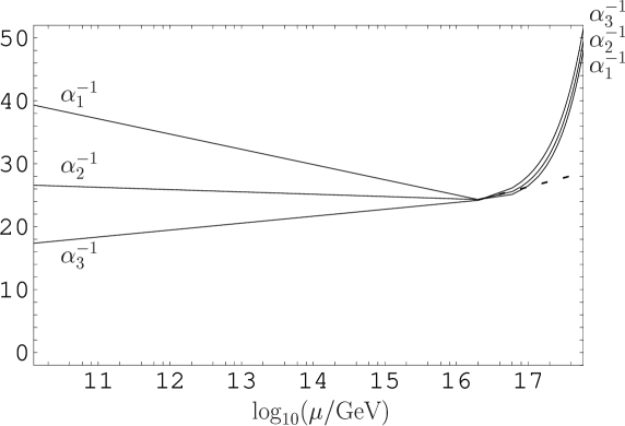
Figure 4: Energy dependence of gauge couplings. The input parameters are given by $\alpha^{-1}_{em}=127.906$, $\sin^{2}\theta_{w}=0.2312$ and $\alpha_{3}=0.1187$ at $M_{Z}=91.1876$GeV. $M_{\textrm{\scriptsize SUSY}}=M_{Z}$ and $1/(2R_{5})=2\times 10^{16}$GeV are chosen. The broken line indicates gauge couplings in minimal 4D supersymmetric grand unified model where $X,Y$ gauge bosons, two triplet Higgs fields and their superpartners in addition to MSSM particles and lead to the coefficient of the $\beta$ function $b_{1}=b_{2}=b_{3}=-8$.

The coupling constants strengthen asymptotic freedom compared to the minimal 4D unified model. This is because in the coefficients of $\beta$ function (3.20) and (3.24), negative contributions by the vector multiplet dominate.

As seen from Tables 6 and 13, the quantum numbers

$$(3,1,-1/3)\oplus(3^{*},1,1/3)\oplus(1,2,1/2)\oplus(1,2,-1/2).$$ (5.53)

appear commonly in all of the 4D unified model and the models with Higgs fields in 5D and in 6D. On the other hand, a way of counting in the coefficients of $\beta$ function depends on the models. In the 4D unified model, they are regarded as one complex scalar and one two-component Weyl fermion. In counting of KK mode contributions in the model with 5D Higgs, they are regarded as two complex scalar and one Dirac fermion. In counting of KK mode contributions in the model with Higgs fields in the 6D gauge multiplet, they are regarded as one vector, one Dirac fermion, one complex scalar. These give rise to the difference of the coefficients of $\beta$ function.

Like the model with 5D Higgs, for gauge couplings, successful SU(5) relations are available. Energy dependence of gauge coupling constants are shown in Fig. 4, where the parameters are the same as that of the model with 5D Higgs. Beyond the unification scale, gauge couplings become asymptotic free more rapidly compared to the 4D unified model. Requiring that this model to be valid may put an upper bound to the scale $1/R_{6}$.

5.3 Yukawa couplings

As in the model with Higgs fields as 5D supermultiplets, $R_{5}$, $R_{6}$ and $g$ are restricted also in the model with Higgs fields in the 6D gauge multiplet. Unlike the model with 5D Higgs, the Yukawa couplings are obtained from the gauge interaction $2\textrm{Re}\left[\Phi_{l}^{c}\Sigma_{5}\Phi_{l}\right]_{F}$ in (2.51) with properties of components shown in Table 2. The neutrino Yukawa interactions arise from $N^{c}\Sigma_{5}N$. For the superfield $N$, the component with the quantum number $(1,1,0,-15p)$ has the parity $(++)$. For $N^{c}$, $N^{c}_{l^{\prime}}$ has the parity $(++)$. Then the interaction which induces the Yukawa coupling is

$$N_{l^{\prime}}^{c(++)}\Sigma_{5~{}(1,2,{1\over 2},18p)}N_{n}^{(++)}.$$ (5.54)

The superfield $\Sigma_{5}\,{}_{(1,2,{1\over 2},18p)}$ has the parity $(++++)$. This zero mode is the Higgs superfield for which the vacuum expectation value $v_{2}$ is developed. For $E$, $E_{u}$ and $E_{e}$ have the parity $(++)$. For $E^{c}$, $E^{c}_{l}$ has the parity $(++)$. The operator ($E^{c(++)}_{L}E_{U}^{(++)}$) has the quantum number $(3^{*},2,-{7\over 6},18p)$ and cannot be coupled to any component of $\Sigma_{5}$. The Yukawa interaction arises from the term with the component $E_{e}$

$$E_{l}^{c(++)}\Sigma_{5~{}(1,2,-{1\over 2},-18p)}^{(++++)}E_{e}^{(++)}.$$ (5.55)

The superfield $\Sigma_{5}\,{}_{(1,2,-{1\over 2},18p)}$ is the other component with the parity $(++++)$ among components of $\Sigma_{5}$. This zero mode is the Higgs superfield for which the vacuum expectation value $v_{1}$ is developed. For $U^{c}$, the component with the parity $(++)$ is $U_{q^{\prime}}^{c\,(++)}$. For $U$, $U_{u^{\prime}}^{(++)}$ and $U_{e^{\prime}}^{(++)}$ have the parity $(++)$. The operator $(U_{q^{\prime}}^{c\,(++)}U_{e^{\prime}}^{(++)})$ does not have its coupling to $\Sigma_{5}$. The possible interaction is

$$U_{q^{\prime}}^{c(++)}\Sigma_{5~{}(1,2,{1\over 2},18p)}^{(++++)}U_{u^{\prime}}^{(++)}.$$ (5.56)

For $D^{c}$ and $D$, $D_{q}^{c}$ and $D_{d}$ have the parity $(++)$. The interaction is

$$D_{q}^{c(++)}\Sigma_{5~{}(1,2,-{1\over 2},-18p)}^{(++++)}D_{d}^{(++)}.$$ (5.57)

For quark sector, the Yukawa interactions are given by

$$\int d^{6}x\delta(x^{6}-\pi R_{6})\,2\textrm{Re}\left[U_{q^{\prime}\,\jmath}^{c}\Sigma_{5}U_{u^{\prime}\,\jmath}+D_{q\,\jmath}^{c}\Sigma_{5}D_{d\jmath}\right]_{F},$$ (5.58)

where generation indices are denoted as $\jmath=1,2,3$. The interactions are diagonal in flavor space. From Eq.(5.44), the fields $U_{q^{\prime}}^{c}$ and $D_{q}^{c}$ is written in terms of $q$. With the notation of zero modes given in Table 12 and the product of mode functions (2.71), Eq.(5.58) leads to the zero mode Yukawa interaction

$$\int d^{6}x\delta(x^{6}-\pi R_{6})\left(q_{\imath}g_{0U\jmath}^{(++)}U_{3\imath\jmath}\Sigma_{5(1,2,\textrm{${1\over 2}$})}u_{\jmath}^{c}f_{0U\jmath}^{(++)}+q_{\imath}g_{0D\jmath}^{(++)}U_{4\imath\jmath}\Sigma_{5(1,2,\textrm{$-{1\over 2}$})}d_{\jmath}^{c}f_{0D\jmath}^{(++)}\right)$$ (5.59)

$$\!\!\!=\!\!\! \int d^{4}x\left({\pi R_{5}M_{U\jmath}\over\sinh(\pi R_{5}M_{U\jmath})}q_{\imath}U_{3\,\imath\jmath}\Sigma_{5(1,2,\textrm{${1\over 2}$})}u_{\jmath}^{c}+{\pi R_{5}M_{D\jmath}\over\sinh(\pi R_{5}M_{D\jmath})}q_{\imath}U_{4\,\imath\jmath}\Sigma_{5(1,2,\textrm{$-{1\over 2}$})}d_{\jmath}^{c}\right),$$

with Hermitian conjugate terms added. From this equation, quark masses at the energy scale $1/2R_{5}$ are obtained as

$$(\textrm{diag}(m_{u},m_{c},m_{t}))_{\jmath_{1}\jmath_{2}} \!\!\!=\!\!\! g_{4D}v_{2}(V_{uL}^{\dagger})_{\jmath_{1}\imath}U_{3\,\imath\jmath}{\pi R_{5}M_{U\jmath}\over\sinh(\pi R_{5}M_{U\jmath})}(V_{uR})_{\jmath\jmath_{2}}$$ (5.60)

$$(\textrm{diag}(m_{d},m_{s},m_{b}))_{\jmath_{1}\jmath_{2}} \!\!\!=\!\!\! g_{4D}v_{1}(V_{dL}^{\dagger})_{\jmath_{1}\imath}U_{4\,\imath\jmath}{\pi R_{5}M_{D\jmath}\over\sinh(\pi R_{5}M_{D\jmath})}(V_{dR})_{\jmath\jmath_{2}}.$$ (5.61)

where $V_{uL}$, $V_{uR}$, $V_{dL}$ and $V_{dR}$ are mixing matrices for quarks. When the kinetic terms for Higgs fields are canonically normalized, $g_{4D}$ appears. The Cabibbo-Kobayashi-Maskawa matrix is obtained as $V_{\textrm{\scriptsize CKM}}=V_{uL}^{\dagger}V_{dL}$. From these equations, 5D masses of fields confined on fixed lines are estimated. For simplicity we choose

$$U_{3}=V_{uL}V_{dL}^{\dagger},\quad~{}U_{4}=V_{dL}V_{dR}^{{\dagger}}.$$ (5.62)

For $\textrm{tan}\beta=10$, $\alpha_{X}^{-1}=24.3$ and $v=\sqrt{2}\times 174.1$GeV, we obtain the 5D masses of up-type and down-type quarks for each generation as

$$M_{U1}=-10,~{}~{}M_{U2}=-6,~{}~{}M_{U3}=-0.9,~{}~{}M_{D1}=-8,~{}~{}M_{D2}=-6,~{}~{}M_{D3}=-3,$$ (5.63)

in unit of $1/(2R_{5})$ by comparing data shown in Table 7. The mass hierarchy is generated due to exponential factor. Since $|M_{U3}|<1/(2R_{5})$ as well as $|M_{U\jmath}|,|M_{D\jmath}|\leq 1/(2R_{6})$ for $R_{6}=R_{5}/10$, KK modes of matter affect gauge coupling correction analyzed in Section 5.2. Since the effect of matter on $\beta$ function are positive for $b$, the inclusion of the KK modes would weaken enhancement of $\alpha^{-1}(\mu)$.

For lepton sector the masses and mixing angles are obtained in a parallel way. From Eq.(5.48), the lepton masses at the energy scale $1/(2R_{5})$ are obtained as

$$(\textrm{diag}(m_{\nu_{e}},m_{\nu_{\mu}},m_{\nu_{\tau}}))_{\jmath_{1}\jmath_{2}} \!\!\!=\!\!\! g_{4D}v_{2}(V_{nL}^{\dagger})_{\jmath_{1}\imath}U_{7\,\imath\jmath}{\pi R_{5}M_{N\jmath}\over\sinh(\pi R_{5}M_{N\jmath})}(V_{nR})_{\jmath\jmath_{2}}$$ (5.64)

$$(\textrm{diag}(m_{e},m_{\mu},m_{\tau}))_{\jmath_{1}\jmath_{2}} \!\!\!=\!\!\! g_{4D}v_{1}(V_{eL}^{\dagger})_{\jmath_{1}\imath}U_{8\,\imath\jmath}{\pi R_{5}M_{E\jmath}\over\sinh(\pi R_{5}M_{E\jmath})}(V_{eR})_{\jmath\jmath_{2}}.$$ (5.65)

where $V_{nL}$, $V_{nR}$, $V_{eL}$ and $V_{eR}$ are mixing matrices for quarks. Small Dirac neutrino masses are obtained via exponential suppression. A small mass such as $10^{-3}$eV is generated by 5D negative mass of the order of $10/R_{5}$. For $\tan\beta$, $\alpha_{X}^{-1}$ and $v$ given above, we obtain the 5D masses of charged leptons for each generation as

$$M_{E1}=-9,~{}~{}M_{E2}=-5,~{}~{}M_{E3}=-3,$$ (5.66)

in unit of $1/(2R_{5})$ for $U_{8}=V_{eL}V_{eR}^{\dagger}$. The mass hierarchy is generated due to exponential factor. Since $|M_{E\jmath}|\leq 1/(2R_{6})$ for $R_{6}=R_{5}/10$, these KK modes also affect gauge coupling correction analyzed in Section 5.2. Since these effects on $\beta$ function is positive for $b$, the inclusion of the KK modes would weaken enhancement of $\alpha^{-1}(\mu)$.

5.4 Proton stability

As in the model with Higgs superfields as 5D supermultiplets, baryon-number violating operators appear also in the model with Higgs superfields in the 6D gauge multiplet. As superpotentials on fixed points, there can be operators to generate dimension-five baryon number violating processes such as

$$U_{T^{\prime}}^{c}U_{T^{\prime}}^{c}U_{T^{\prime}}^{c}E_{F}^{c}\approx(TU_{3})(TU_{3})(TU_{3})(FU_{8}),$$ (5.67)

where Eqs(5.34) and (5.47) have been used and $\approx$ denotes equivalence except for decoupled heavy fields. The operator (5.67) corresponds to the first operator in Eq.(4.121) in the model with Higgs superfields as 5D supermultiplets. Such operators are forbidden by R invariance with charges assigned in Table 14.

Table 14: R-charges in model with Higgs in gauge multiplet.

$\theta$	$V$, $\Sigma_{5}$, $\Sigma_{6}$	$\Phi$	$D$, $D^{c}$, $U$, $U^{c}$, $E$, $E^{c}$, $N$, $N^{c}$	$\bar{T}$	$S$	${\cal X}$	${\cal B}$, $\bar{\cal B}$
$-1$	0	2	1	1	0	2	0

In addition, the dimension-six proton decay by colored Higgs exchange is absent unlike the model with Higgs fields as 5D chiral superfields, while the dimension-six proton decay by $X$ and $Y$ boson exchange would exist.

5.5 Supersymmetry breaking

The two MSSM Higgs fields which are part of the 6D gauge multiplet propagate in 6D. One may expect that the Higgs superfields would be directly coupled to supersymmetry breaking source as

$$2\textrm{Re}\left[{1\over M}SW^{\alpha}W_{\alpha}\right]_{F}$$

$$+{1\over 2}\left[\left(\left({1\over M}S^{\dagger}+{1\over M^{2}}S^{\dagger}S\right)H_{1}H_{2}+\textrm{H.c.}\right)+{1\over M^{2}}S^{\dagger}S\left(H_{1}^{\dagger}H_{1}+H_{2}^{\dagger}H_{2}\right)\right]_{D},$$ (5.68)

at $(x^{5},x^{6})=(\pi R_{5},0)$. Such couplings appeared in gaugino mediation with the standard model gauge fields and Higgs fields and their superpartners in bulk [13]. If the coupling

$$S^{\dagger}S\textrm{Tr}(\Sigma_{5}^{\dagger}\Sigma_{5})=S^{\dagger}S(H_{1}^{\dagger}H_{1}+H_{2}^{\dagger}H_{2})+\cdots,$$ (5.69)

is allowed, the coupling seems to lead to Higgs mass terms. At the fixed point $(\pi R_{5},0)$, restricted gauge symmetry has SU(4)$\times$ SU(2)$\times$U(1). The field $\Sigma_{5}$ is written as

$$\Sigma_{5}\bigg{|}_{(\pi R_{5},0)}=\left(\begin{array}[]{c|c}\Sigma_{2\cdot 2}&\Sigma_{2\cdot 4}\\ \hline\cr\Sigma_{4\cdot 2}&\Sigma_{4\cdot 4}\\ \end{array}\right).$$ (5.72)

If the coupling

$$S^{\dagger}\textrm{Tr}(\Sigma_{2\cdot 4}\Sigma_{4\cdot 2})=S^{\dagger}H_{1}H_{2}+\cdots$$ (5.73)

is allowed, this seems $\mu$ term. However, the operators $\textrm{Tr}(\Sigma_{5}^{\dagger}\Sigma_{5})$ and $\textrm{Tr}(\Sigma_{2\times 4}\Sigma_{4\times 2})$ are gauge non-invariant due to $\partial_{5}$-factor of the transformation (2.8)

$$\Sigma_{5}\to\Sigma_{5}^{\prime}=e^{-\Lambda}(\partial_{5}+\Sigma_{5})e^{\Lambda}.$$ (5.74)

Thus in this model, Higgs masses and $\mu$ and $B\mu$ terms are not generated by contact interactions. At $\mu=M_{X}$ the model has nonzero gaugino mass and negligible soft scalar mass.

For electroweak symmetry breaking, the quartic terms of Higgs doublet appear from $D$-term. In the operator (2.18), they are included in the term $-({\cal D}^{N}\varphi)^{*}({\cal D}_{N}\varphi)$. Since there is no term such as Eq.(5.68), $\mu$ term must be generated via other mechanism. In case with Chern-Simons terms, it was proposed that combining $F$-components of compensator and radion as well as constant superpotentials can generate $\mu$ term [27]. In this mechanism, nontrivial radion potential is crucial. It has also been shown that a potential of radion with radius stabilization is generated in a model with compensator, radion and constant superpotentials [28][29] and that this radius stabilization is sensitive to field content [30]. Whether a radion potential relevant to generation of $\mu$ term arises in the present models is an open problem.

6 Conclusion

We have studied gauge coupling corrections and Yukawa coupling constants in 6D unified models based on the gauge group SU(6). For a possibility of gauge-Higgs unification and inclusion of right-handed neutrino, gauge group larger than the standard model gauge group has been motivated. We have employed two extra dimensions to approach the doublet-triplet splitting, no fermion mass relations for the first two generations and gaugino-mediated supersymmetry breaking (no supersymmetry flavor problem). The source of supersymmetry breaking is spatially separated from fixed lines and fixed points where matter fields reside. By orbifold, theory on fixed lines and fixed points has restricted gauge symmetry. Heavy fields decouple by boundary conditions. The models are 6D and 4D anomaly free and proton stability is achieved by R invariance as a subgroup of SU(2)${}_{\textrm{\scriptsize R}}$.

For energy dependence of gauge coupling constants, we have adopted 4D KK effective theory by giving a 6D component action and the fixed-line and fixed-point actions. The number of KK mode is regarded as energy-dependent. At each scale $1/(2R_{5})$, $1/R_{5}$, $3/(2R_{5})$, $\cdots$, 4D KK states with the corresponding masses become dynamical. For the effective 4D theory, restricted gauge invariance has the gauge group SU(3)${}_{\textrm{\scriptsize C}}$$\times$ SU(2)${}_{\textrm{\scriptsize W}}$$\times$U(1)_Y$\times$U(1)^′. The gauge group U(1)^′ is spontaneously broken by fixed-point couplings. Up to the unification scale, zero mode contributes to renormalization group evolution. Since zero mode is right-handed neutrino and its superpartner as well as the field content of MSSM, successful SU(5) relations about the gauge coupling unification, weak mixing angle and charge quantization have been achieved. Beyond the unification scale, gauge couplings are sensitive to the field content. In the model with 5D Higgs, the sum of the coefficients of $\beta$ function relevant to KK mode is $b_{(1)}+b_{(2)}=4$ independently of gauge group. This leads to strong coupling at high energies. In the model with the Higgs superfields in the 6D gauge multiplet, $b_{(1)}+b_{(2)}=-12$. Asymptotic freedom is more strong compared to the 4D unified model. These rapid energy dependence is likely to constrain the scale $1/R_{6}$. In the two models, it may be chosen as $1/R_{6}<M_{Pl}$. For $1/(2R_{5})=M_{X}$, $1/R_{6}<M_{Pl}$ and $\alpha_{X}^{-1}=24.3$, realistic patterns of Yukawa couplings have been obtained from fixed-point coupling in the model with 5D Higgs fields and from the gauge interaction in the model with Higgs fields in the 6D gauge multiplet. For the values of paramters, small numbers required for the hierarchy of Yukawa coupling constants have been generated via volume suppression in the model with 5D Higgs fields and exponential suppression dependent on 5D masses in the model with Higgs fields in the gauge multiplet.

We have fixed the smaller compactification radius $1/(2R_{5})=M_{X}$. From a viewpoint of LSP, it may be important to examine the case $1/(2R_{5})\neq M_{X}$ in a 6D setup where no fermion mass relations for the first two generations and gaugino-mediated supersymmetry breaking still hold. Gaugino masses as an input at high energies influence the whole values of supersymmetry breaking masses. For a large $M_{1/2}$, spectrum avoiding the lightest stau as LSP was obtained for a moderate $\tan\beta$ and for $1/(2R_{5})\neq M_{X}$ [31]. In models with the two extra dimensions radiative correction may also affect spectrum [32]. There is still room to be examined about this point.

Acknowledgments

I thank Masud Chaichian, Nobuhito Maru and Norisuke Sakai for useful discussions. This work is supported by Bilateral exchange program between Japan Society for the Promotion of Science and the Academy of Finland.

Appendix A SU(6) group and 6D spinor

A.1 SU(6) generators and structure constants

The generators of SU(6) transformations, $\lambda_{a}$ ($a=1,\cdots 35$) are

$$\!\!\!\!\!\!\!\!\lambda_{1}\!\!=\!\!\left(\!\begin{array}[]{cccccc}{}^{\cdot}_{1}\!&\!{}^{1}_{\cdot}\!&\!{}^{\cdot}_{\cdot}\!&\!{}^{\cdot}_{\cdot}\!&\!{}^{\cdot}_{\cdot}\!&\!{}^{\cdot}_{\cdot}\\ {}^{\cdot}_{\cdot}\!&\!{}^{\cdot}_{\cdot}\!&\!{}^{\cdot}_{\cdot}\!&\!{}^{\cdot}_{\cdot}\!&\!{}^{\cdot}_{\cdot}\!&\!{}^{\cdot}_{\cdot}\\ {}^{\cdot}_{\cdot}\!&\!{}^{\cdot}_{\cdot}\!&\!{}^{\cdot}_{\cdot}\!&\!{}^{\cdot}_{\cdot}\!&\!{}^{\cdot}_{\cdot}\!&\!{}^{\cdot}_{\cdot}\\ \end{array}\!\right)\!\!,~{}\lambda_{2}\!\!=\!\!\left(\!\begin{array}[]{cccccc}{}^{\cdot}_{i}\!&\!{}^{-i}_{~{}\cdot}\!&\!{}^{\cdot}_{\cdot}\!&\!{}^{\cdot}_{\cdot}\!&\!{}^{\cdot}_{\cdot}\!&\!{}^{\cdot}_{\cdot}\\ {}^{\cdot}_{\cdot}\!&\!{}^{\cdot}_{\cdot}\!&\!{}^{\cdot}_{\cdot}\!&\!{}^{\cdot}_{\cdot}\!&\!{}^{\cdot}_{\cdot}\!&\!{}^{\cdot}_{\cdot}\\ {}^{\cdot}_{\cdot}\!&\!{}^{\cdot}_{\cdot}\!&\!{}^{\cdot}_{\cdot}\!&\!{}^{\cdot}_{\cdot}\!&\!{}^{\cdot}_{\cdot}\!&\!{}^{\cdot}_{\cdot}\\ \end{array}\!\right)\!\!,~{}\lambda_{3}\!\!=\!\!\left(\!\begin{array}[]{cccccc}{}^{1}_{\cdot}\!&\!{}^{~{}\cdot}_{-1}\!&\!{}^{\cdot}_{\cdot}\!&\!{}^{\cdot}_{\cdot}\!&\!{}^{\cdot}_{\cdot}\!&\!{}^{\cdot}_{\cdot}\\ {}^{\cdot}_{\cdot}\!&\!{}^{\cdot}_{\cdot}\!&\!{}^{\cdot}_{\cdot}\!&\!{}^{\cdot}_{\cdot}\!&\!{}^{\cdot}_{\cdot}\!&\!{}^{\cdot}_{\cdot}\\ {}^{\cdot}_{\cdot}\!&\!{}^{\cdot}_{\cdot}\!&\!{}^{\cdot}_{\cdot}\!&\!{}^{\cdot}_{\cdot}\!&\!{}^{\cdot}_{\cdot}\!&\!{}^{\cdot}_{\cdot}\\ \end{array}\!\right)\!\!,~{}\lambda_{4}\!\!=\!\!\left(\!\begin{array}[]{cccccc}{}^{\cdot}_{\cdot}\!&\!{}^{\cdot}_{\cdot}\!&\!{}^{1}_{\cdot}\!&\!{}^{\cdot}_{\cdot}\!&\!{}^{\cdot}_{\cdot}\!&\!{}^{\cdot}_{\cdot}\\ {}^{1}_{\cdot}\!&\!{}^{\cdot}_{\cdot}\!&\!{}^{\cdot}_{\cdot}\!&\!{}^{\cdot}_{\cdot}\!&\!{}^{\cdot}_{\cdot}\!&\!{}^{\cdot}_{\cdot}\\ {}^{\cdot}_{\cdot}\!&\!{}^{\cdot}_{\cdot}\!&\!{}^{\cdot}_{\cdot}\!&\!{}^{\cdot}_{\cdot}\!&\!{}^{\cdot}_{\cdot}\!&\!{}^{\cdot}_{\cdot}\\ \end{array}\!\right)\!\!,~{}$$

$$\!\!\!\!\!\!\!\!\lambda_{5}\!\!=\!\!\left(\!\begin{array}[]{cccccc}{}^{\cdot}_{\cdot}\!&\!{}^{\cdot}_{\cdot}\!&\!{}^{-i}_{~{}\cdot}\!&\!{}^{\cdot}_{\cdot}\!&\!{}^{\cdot}_{\cdot}\!&\!{}^{\cdot}_{\cdot}\\ {}^{i}_{\cdot}\!&\!{}^{\cdot}_{\cdot}\!&\!{}^{\cdot}_{\cdot}\!&\!{}^{\cdot}_{\cdot}\!&\!{}^{\cdot}_{\cdot}\!&\!{}^{\cdot}_{\cdot}\\ {}^{\cdot}_{\cdot}\!&\!{}^{\cdot}_{\cdot}\!&\!{}^{\cdot}_{\cdot}\!&\!{}^{\cdot}_{\cdot}\!&\!{}^{\cdot}_{\cdot}\!&\!{}^{\cdot}_{\cdot}\\ \end{array}\!\right)\!\!,~{}~{}\lambda_{6}\!\!=\!\!\left(\!\begin{array}[]{cccccc}{}^{\cdot}_{\cdot}\!&\!{}^{\cdot}_{\cdot}\!&\!{}^{\cdot}_{1}\!&\!{}^{\cdot}_{\cdot}\!&\!{}^{\cdot}_{\cdot}\!&\!{}^{\cdot}_{\cdot}\\ {}^{\cdot}_{\cdot}\!&\!{}^{1}_{\cdot}\!&\!{}^{\cdot}_{\cdot}\!&\!{}^{\cdot}_{\cdot}\!&\!{}^{\cdot}_{\cdot}\!&\!{}^{\cdot}_{\cdot}\\ {}^{\cdot}_{\cdot}\!&\!{}^{\cdot}_{\cdot}\!&\!{}^{\cdot}_{\cdot}\!&\!{}^{\cdot}_{\cdot}\!&\!{}^{\cdot}_{\cdot}\!&\!{}^{\cdot}_{\cdot}\\ \end{array}\!\right)\!\!,~{}~{}\lambda_{7}\!\!=\!\!\left(\!\begin{array}[]{cccccc}{}^{\cdot}_{\cdot}\!&\!{}^{\cdot}_{\cdot}\!&\!{}^{~{}\cdot}_{-i}\!&\!{}^{\cdot}_{\cdot}\!&\!{}^{\cdot}_{\cdot}\!&\!{}^{\cdot}_{\cdot}\\ {}^{\cdot}_{\cdot}\!&\!{}^{i}_{\cdot}\!&\!{}^{\cdot}_{\cdot}\!&\!{}^{\cdot}_{\cdot}\!&\!{}^{\cdot}_{\cdot}\!&\!{}^{\cdot}_{\cdot}\\ {}^{\cdot}_{\cdot}\!&\!{}^{\cdot}_{\cdot}\!&\!{}^{\cdot}_{\cdot}\!&\!{}^{\cdot}_{\cdot}\!&\!{}^{\cdot}_{\cdot}\!&\!{}^{\cdot}_{\cdot}\\ \end{array}\!\right)\!\!,~{}~{}$$

$$\!\!\!\!\!\!\!\!\lambda_{8}\!\!=\!\!\textrm{${1\over\sqrt{3}}$}\left(\!\begin{array}[]{cccccc}{}^{1}_{\cdot}\!&\!{}^{\cdot}_{1}\!&\!{}^{\cdot}_{\cdot}\!&\!{}^{\cdot}_{\cdot}\!&\!{}^{\cdot}_{\cdot}\!&\!{}^{\cdot}_{\cdot}\\ {}^{\cdot}_{\cdot}\!&\!{}^{\cdot}_{\cdot}\!&\!{}^{-2}_{~{}\cdot}\!&\!{}^{\cdot}_{\cdot}\!&\!{}^{\cdot}_{\cdot}\!&\!{}^{\cdot}_{\cdot}\\ {}^{\cdot}_{\cdot}\!&\!{}^{\cdot}_{\cdot}\!&\!{}^{\cdot}_{\cdot}\!&\!{}^{\cdot}_{\cdot}\!&\!{}^{\cdot}_{\cdot}\!&\!{}^{\cdot}_{\cdot}\\ \end{array}\!\right)\!\!,~{}~{}\lambda_{9}\!\!=\!\!\left(\!\begin{array}[]{cccccc}{}^{\cdot}_{\cdot}\!&\!{}^{\cdot}_{\cdot}\!&\!{}^{\cdot}_{\cdot}\!&\!{}^{1}_{\cdot}\!&\!{}^{\cdot}_{\cdot}\!&\!{}^{\cdot}_{\cdot}\\ {}^{\cdot}_{1}\!&\!{}^{\cdot}_{\cdot}\!&\!{}^{\cdot}_{\cdot}\!&\!{}^{\cdot}_{\cdot}\!&\!{}^{\cdot}_{\cdot}\!&\!{}^{\cdot}_{\cdot}\\ {}^{\cdot}_{\cdot}\!&\!{}^{\cdot}_{\cdot}\!&\!{}^{\cdot}_{\cdot}\!&\!{}^{\cdot}_{\cdot}\!&\!{}^{\cdot}_{\cdot}\!&\!{}^{\cdot}_{\cdot}\\ \end{array}\!\right)\!\!,~{}~{}\lambda_{10}\!\!=\!\!\left(\!\begin{array}[]{cccccc}{}^{\cdot}_{\cdot}\!&\!{}^{\cdot}_{\cdot}\!&\!{}^{\cdot}_{\cdot}\!&\!{}^{-i}_{~{}\cdot}\!&\!{}^{\cdot}_{\cdot}\!&\!{}^{\cdot}_{\cdot}\\ {}^{\cdot}_{i}\!&\!{}^{\cdot}_{\cdot}\!&\!{}^{\cdot}_{\cdot}\!&\!{}^{\cdot}_{\cdot}\!&\!{}^{\cdot}_{\cdot}\!&\!{}^{\cdot}_{\cdot}\\ {}^{\cdot}_{\cdot}\!&\!{}^{\cdot}_{\cdot}\!&\!{}^{\cdot}_{\cdot}\!&\!{}^{\cdot}_{\cdot}\!&\!{}^{\cdot}_{\cdot}\!&\!{}^{\cdot}_{\cdot}\\ \end{array}\!\right)\!\!,~{}~{}$$

$$\!\!\!\!\!\!\!\!\lambda_{11}\!\!=\!\!\left(\!\begin{array}[]{cccccc}{}^{\cdot}_{\cdot}\!&\!{}^{\cdot}_{\cdot}\!&\!{}^{\cdot}_{\cdot}\!&\!{}^{\cdot}_{1}\!&\!{}^{\cdot}_{\cdot}\!&\!{}^{\cdot}_{\cdot}\\ {}^{\cdot}_{\cdot}\!&\!{}^{\cdot}_{1}\!&\!{}^{\cdot}_{\cdot}\!&\!{}^{\cdot}_{\cdot}\!&\!{}^{\cdot}_{\cdot}\!&\!{}^{\cdot}_{\cdot}\\ {}^{\cdot}_{\cdot}\!&\!{}^{\cdot}_{\cdot}\!&\!{}^{\cdot}_{\cdot}\!&\!{}^{\cdot}_{\cdot}\!&\!{}^{\cdot}_{\cdot}\!&\!{}^{\cdot}_{\cdot}\\ \end{array}\!\right)\!\!,~{}\lambda_{12}\!\!=\!\!\left(\!\begin{array}[]{cccccc}{}^{\cdot}_{\cdot}\!&\!{}^{\cdot}_{\cdot}\!&\!{}^{\cdot}_{\cdot}\!&\!{}^{~{}\cdot}_{-i}\!&\!{}^{\cdot}_{\cdot}\!&\!{}^{\cdot}_{\cdot}\\ {}^{\cdot}_{\cdot}\!&\!{}^{\cdot}_{i}\!&\!{}^{\cdot}_{\cdot}\!&\!{}^{\cdot}_{\cdot}\!&\!{}^{\cdot}_{\cdot}\!&\!{}^{\cdot}_{\cdot}\\ {}^{\cdot}_{\cdot}\!&\!{}^{\cdot}_{\cdot}\!&\!{}^{\cdot}_{\cdot}\!&\!{}^{\cdot}_{\cdot}\!&\!{}^{\cdot}_{\cdot}\!&\!{}^{\cdot}_{\cdot}\\ \end{array}\!\right)\!\!,~{}\lambda_{13}\!\!=\!\!\left(\!\begin{array}[]{cccccc}{}^{\cdot}_{\cdot}\!&\!{}^{\cdot}_{\cdot}\!&\!{}^{\cdot}_{\cdot}\!&\!{}^{\cdot}_{\cdot}\!&\!{}^{\cdot}_{\cdot}\!&\!{}^{\cdot}_{\cdot}\\ {}^{\cdot}_{\cdot}\!&\!{}^{\cdot}_{\cdot}\!&\!{}^{\cdot}_{1}\!&\!{}^{1}_{\cdot}\!&\!{}^{\cdot}_{\cdot}\!&\!{}^{\cdot}_{\cdot}\\ {}^{\cdot}_{\cdot}\!&\!{}^{\cdot}_{\cdot}\!&\!{}^{\cdot}_{\cdot}\!&\!{}^{\cdot}_{\cdot}\!&\!{}^{\cdot}_{\cdot}\!&\!{}^{\cdot}_{\cdot}\\ \end{array}\!\right)\!\!,~{}\lambda_{14}\!\!=\!\!\left(\!\begin{array}[]{cccccc}{}^{\cdot}_{\cdot}\!&\!{}^{\cdot}_{\cdot}\!&\!{}^{\cdot}_{\cdot}\!&\!{}^{\cdot}_{\cdot}\!&\!{}^{\cdot}_{\cdot}\!&\!{}^{\cdot}_{\cdot}\\ {}^{\cdot}_{\cdot}\!&\!{}^{\cdot}_{\cdot}\!&\!{}^{\cdot}_{i}\!&\!{}^{-i}_{~{}\cdot}\!&\!{}^{\cdot}_{\cdot}\!&\!{}^{\cdot}_{\cdot}\\ {}^{\cdot}_{\cdot}\!&\!{}^{\cdot}_{\cdot}\!&\!{}^{\cdot}_{\cdot}\!&\!{}^{\cdot}_{\cdot}\!&\!{}^{\cdot}_{\cdot}\!&\!{}^{\cdot}_{\cdot}\\ \end{array}\!\right)\!\!,~{}$$

$$\!\!\!\!\!\!\!\!\lambda_{15}\!\!=\!\!\textrm{${1\over\sqrt{6}}$}\left(\!\begin{array}[]{cccccc}{}^{1}_{\cdot}\!&\!{}^{\cdot}_{1}\!&\!{}^{\cdot}_{\cdot}\!&\!{}^{\cdot}_{\cdot}\!&\!{}^{\cdot}_{\cdot}\!&\!{}^{\cdot}_{\cdot}\\ {}^{\cdot}_{\cdot}\!&\!{}^{\cdot}_{\cdot}\!&\!{}^{1}_{\cdot}\!&\!{}^{~{}\cdot}_{-3}\!&\!{}^{\cdot}_{\cdot}\!&\!{}^{\cdot}_{\cdot}\\ {}^{\cdot}_{\cdot}\!&\!{}^{\cdot}_{\cdot}\!&\!{}^{\cdot}_{\cdot}\!&\!{}^{\cdot}_{\cdot}\!&\!{}^{\cdot}_{\cdot}\!&\!{}^{\cdot}_{\cdot}\\ \end{array}\!\right)\!\!,~{}~{}\lambda_{16}\!\!=\!\!\left(\!\begin{array}[]{cccccc}{}^{\cdot}_{\cdot}\!&\!{}^{\cdot}_{\cdot}\!&\!{}^{\cdot}_{\cdot}\!&\!{}^{\cdot}_{\cdot}\!&\!{}^{1}_{\cdot}\!&\!{}^{\cdot}_{\cdot}\\ {}^{\cdot}_{\cdot}\!&\!{}^{\cdot}_{\cdot}\!&\!{}^{\cdot}_{\cdot}\!&\!{}^{\cdot}_{\cdot}\!&\!{}^{\cdot}_{\cdot}\!&\!{}^{\cdot}_{\cdot}\\ {}^{1}_{\cdot}\!&\!{}^{\cdot}_{\cdot}\!&\!{}^{\cdot}_{\cdot}\!&\!{}^{\cdot}_{\cdot}\!&\!{}^{\cdot}_{\cdot}\!&\!{}^{\cdot}_{\cdot}\\ \end{array}\!\right)\!\!,~{}~{}\lambda_{17}\!\!=\!\!\left(\!\begin{array}[]{cccccc}{}^{\cdot}_{\cdot}\!&\!{}^{\cdot}_{\cdot}\!&\!{}^{\cdot}_{\cdot}\!&\!{}^{\cdot}_{\cdot}\!&\!{}^{-i}_{~{}\cdot}\!&\!{}^{\cdot}_{\cdot}\\ {}^{\cdot}_{\cdot}\!&\!{}^{\cdot}_{\cdot}\!&\!{}^{\cdot}_{\cdot}\!&\!{}^{\cdot}_{\cdot}\!&\!{}^{\cdot}_{\cdot}\!&\!{}^{\cdot}_{\cdot}\\ {}^{i}_{\cdot}\!&\!{}^{\cdot}_{\cdot}\!&\!{}^{\cdot}_{\cdot}\!&\!{}^{\cdot}_{\cdot}\!&\!{}^{\cdot}_{\cdot}\!&\!{}^{\cdot}_{\cdot}\\ \end{array}\!\right)\!\!,~{}~{}$$

$$\!\!\!\!\!\!\!\!\lambda_{18}\!\!=\!\!\left(\!\begin{array}[]{cccccc}{}^{\cdot}_{\cdot}\!&\!{}^{\cdot}_{\cdot}\!&\!{}^{\cdot}_{\cdot}\!&\!{}^{\cdot}_{\cdot}\!&\!{}^{\cdot}_{1}\!&\!{}^{\cdot}_{\cdot}\\ {}^{\cdot}_{\cdot}\!&\!{}^{\cdot}_{\cdot}\!&\!{}^{\cdot}_{\cdot}\!&\!{}^{\cdot}_{\cdot}\!&\!{}^{\cdot}_{\cdot}\!&\!{}^{\cdot}_{\cdot}\\ {}^{\cdot}_{\cdot}\!&\!{}^{1}_{\cdot}\!&\!{}^{\cdot}_{\cdot}\!&\!{}^{\cdot}_{\cdot}\!&\!{}^{\cdot}_{\cdot}\!&\!{}^{\cdot}_{\cdot}\\ \end{array}\!\right)\!\!,~{}\lambda_{19}\!\!=\!\!\left(\!\begin{array}[]{cccccc}{}^{\cdot}_{\cdot}\!&\!{}^{\cdot}_{\cdot}\!&\!{}^{\cdot}_{\cdot}\!&\!{}^{\cdot}_{\cdot}\!&\!{}^{~{}\cdot}_{-i}\!&\!{}^{\cdot}_{\cdot}\\ {}^{\cdot}_{\cdot}\!&\!{}^{\cdot}_{\cdot}\!&\!{}^{\cdot}_{\cdot}\!&\!{}^{\cdot}_{\cdot}\!&\!{}^{\cdot}_{\cdot}\!&\!{}^{\cdot}_{\cdot}\\ {}^{\cdot}_{\cdot}\!&\!{}^{i}_{\cdot}\!&\!{}^{\cdot}_{\cdot}\!&\!{}^{\cdot}_{\cdot}\!&\!{}^{\cdot}_{\cdot}\!&\!{}^{\cdot}_{\cdot}\\ \end{array}\!\right)\!\!,~{}\lambda_{20}\!\!=\!\!\left(\!\begin{array}[]{cccccc}{}^{\cdot}_{\cdot}\!&\!{}^{\cdot}_{\cdot}\!&\!{}^{\cdot}_{\cdot}\!&\!{}^{\cdot}_{\cdot}\!&\!{}^{\cdot}_{\cdot}\!&\!{}^{\cdot}_{\cdot}\\ {}^{\cdot}_{\cdot}\!&\!{}^{\cdot}_{\cdot}\!&\!{}^{\cdot}_{\cdot}\!&\!{}^{\cdot}_{\cdot}\!&\!{}^{1}_{\cdot}\!&\!{}^{\cdot}_{\cdot}\\ {}^{\cdot}_{\cdot}\!&\!{}^{\cdot}_{\cdot}\!&\!{}^{1}_{\cdot}\!&\!{}^{\cdot}_{\cdot}\!&\!{}^{\cdot}_{\cdot}\!&\!{}^{\cdot}_{\cdot}\\ \end{array}\!\right)\!\!,~{}\lambda_{21}\!\!=\!\!\left(\!\begin{array}[]{cccccc}{}^{\cdot}_{\cdot}\!&\!{}^{\cdot}_{\cdot}\!&\!{}^{\cdot}_{\cdot}\!&\!{}^{\cdot}_{\cdot}\!&\!{}^{\cdot}_{\cdot}\!&\!{}^{\cdot}_{\cdot}\\ {}^{\cdot}_{\cdot}\!&\!{}^{\cdot}_{\cdot}\!&\!{}^{\cdot}_{\cdot}\!&\!{}^{\cdot}_{\cdot}\!&\!{}^{-i}_{~{}\cdot}\!&\!{}^{\cdot}_{\cdot}\\ {}^{\cdot}_{\cdot}\!&\!{}^{\cdot}_{\cdot}\!&\!{}^{i}_{\cdot}\!&\!{}^{\cdot}_{\cdot}\!&\!{}^{\cdot}_{\cdot}\!&\!{}^{\cdot}_{\cdot}\\ \end{array}\!\right)\!\!,~{}$$

$$\!\!\!\!\!\!\!\!\lambda_{22}\!\!=\!\!\left(\!\begin{array}[]{cccccc}{}^{\cdot}_{\cdot}\!&\!{}^{\cdot}_{\cdot}\!&\!{}^{\cdot}_{\cdot}\!&\!{}^{\cdot}_{\cdot}\!&\!{}^{\cdot}_{\cdot}\!&\!{}^{\cdot}_{\cdot}\\ {}^{\cdot}_{\cdot}\!&\!{}^{\cdot}_{\cdot}\!&\!{}^{\cdot}_{\cdot}\!&\!{}^{\cdot}_{\cdot}\!&\!{}^{\cdot}_{1}\!&\!{}^{\cdot}_{\cdot}\\ {}^{\cdot}_{\cdot}\!&\!{}^{\cdot}_{\cdot}\!&\!{}^{\cdot}_{\cdot}\!&\!{}^{1}_{\cdot}\!&\!{}^{\cdot}_{\cdot}\!&\!{}^{\cdot}_{\cdot}\\ \end{array}\!\right)\!\!,~{}~{}\lambda_{23}\!\!=\!\!\left(\!\begin{array}[]{cccccc}{}^{\cdot}_{\cdot}\!&\!{}^{\cdot}_{\cdot}\!&\!{}^{\cdot}_{\cdot}\!&\!{}^{\cdot}_{\cdot}\!&\!{}^{\cdot}_{\cdot}\!&\!{}^{\cdot}_{\cdot}\\ {}^{\cdot}_{\cdot}\!&\!{}^{\cdot}_{\cdot}\!&\!{}^{\cdot}_{\cdot}\!&\!{}^{\cdot}_{\cdot}\!&\!{}^{~{}\cdot}_{-i}\!&\!{}^{\cdot}_{\cdot}\\ {}^{\cdot}_{\cdot}\!&\!{}^{\cdot}_{\cdot}\!&\!{}^{\cdot}_{\cdot}\!&\!{}^{i}_{\cdot}\!&\!{}^{\cdot}_{\cdot}\!&\!{}^{\cdot}_{\cdot}\\ \end{array}\!\right)\!\!,~{}~{}\lambda_{24}\!\!=\!\!\textrm{${1\over\sqrt{10}}$}\left(\!\begin{array}[]{cccccc}{}^{1}_{\cdot}\!&\!{}^{\cdot}_{1}\!&\!{}^{\cdot}_{\cdot}\!&\!{}^{\cdot}_{\cdot}\!&\!{}^{\cdot}_{\cdot}\!&\!{}^{\cdot}_{\cdot}\\ {}^{\cdot}_{\cdot}\!&\!{}^{\cdot}_{\cdot}\!&\!{}^{1}_{\cdot}\!&\!{}^{\cdot}_{1}\!&\!{}^{\cdot}_{\cdot}\!&\!{}^{\cdot}_{\cdot}\\ {}^{\cdot}_{\cdot}\!&\!{}^{\cdot}_{\cdot}\!&\!{}^{\cdot}_{\cdot}\!&\!{}^{\cdot}_{\cdot}\!&\!{}^{-4}_{~{}\cdot}\!&\!{}^{\cdot}_{\cdot}\\ \end{array}\!\right)\!\!,~{}~{}$$

$$\!\!\!\!\!\!\!\!\lambda_{25}\!\!=\!\!\left(\!\begin{array}[]{cccccc}{}^{\cdot}_{\cdot}\!&\!{}^{\cdot}_{\cdot}\!&\!{}^{\cdot}_{\cdot}\!&\!{}^{\cdot}_{\cdot}\!&\!{}^{\cdot}_{\cdot}\!&\!{}^{1}_{\cdot}\\ {}^{\cdot}_{\cdot}\!&\!{}^{\cdot}_{\cdot}\!&\!{}^{\cdot}_{\cdot}\!&\!{}^{\cdot}_{\cdot}\!&\!{}^{\cdot}_{\cdot}\!&\!{}^{\cdot}_{\cdot}\\ {}^{\cdot}_{1}\!&\!{}^{\cdot}_{\cdot}\!&\!{}^{\cdot}_{\cdot}\!&\!{}^{\cdot}_{\cdot}\!&\!{}^{\cdot}_{\cdot}\!&\!{}^{\cdot}_{\cdot}\\ \end{array}\!\right)\!\!,~{}\lambda_{26}\!\!=\!\!\left(\!\begin{array}[]{cccccc}{}^{\cdot}_{\cdot}\!&\!{}^{\cdot}_{\cdot}\!&\!{}^{\cdot}_{\cdot}\!&\!{}^{\cdot}_{\cdot}\!&\!{}^{\cdot}_{\cdot}\!&\!{}^{-i}_{~{}\cdot}\\ {}^{\cdot}_{\cdot}\!&\!{}^{\cdot}_{\cdot}\!&\!{}^{\cdot}_{\cdot}\!&\!{}^{\cdot}_{\cdot}\!&\!{}^{\cdot}_{\cdot}\!&\!{}^{\cdot}_{\cdot}\\ {}^{\cdot}_{i}\!&\!{}^{\cdot}_{\cdot}\!&\!{}^{\cdot}_{\cdot}\!&\!{}^{\cdot}_{\cdot}\!&\!{}^{\cdot}_{\cdot}\!&\!{}^{\cdot}_{\cdot}\\ \end{array}\!\right)\!\!,~{}\lambda_{27}\!\!=\!\!\left(\!\begin{array}[]{cccccc}{}^{\cdot}_{\cdot}\!&\!{}^{\cdot}_{\cdot}\!&\!{}^{\cdot}_{\cdot}\!&\!{}^{\cdot}_{\cdot}\!&\!{}^{\cdot}_{\cdot}\!&\!{}^{\cdot}_{1}\\ {}^{\cdot}_{\cdot}\!&\!{}^{\cdot}_{\cdot}\!&\!{}^{\cdot}_{\cdot}\!&\!{}^{\cdot}_{\cdot}\!&\!{}^{\cdot}_{\cdot}\!&\!{}^{\cdot}_{\cdot}\\ {}^{\cdot}_{\cdot}\!&\!{}^{\cdot}_{1}\!&\!{}^{\cdot}_{\cdot}\!&\!{}^{\cdot}_{\cdot}\!&\!{}^{\cdot}_{\cdot}\!&\!{}^{\cdot}_{\cdot}\\ \end{array}\!\right)\!\!,~{}~{}\lambda_{28}\!\!=\!\!\left(\!\begin{array}[]{cccccc}{}^{\cdot}_{\cdot}\!&\!{}^{\cdot}_{\cdot}\!&\!{}^{\cdot}_{\cdot}\!&\!{}^{\cdot}_{\cdot}\!&\!{}^{\cdot}_{\cdot}\!&\!{}^{~{}\cdot}_{-i}\\ {}^{\cdot}_{\cdot}\!&\!{}^{\cdot}_{\cdot}\!&\!{}^{\cdot}_{\cdot}\!&\!{}^{\cdot}_{\cdot}\!&\!{}^{\cdot}_{\cdot}\!&\!{}^{\cdot}_{\cdot}\\ {}^{\cdot}_{\cdot}\!&\!{}^{\cdot}_{i}\!&\!{}^{\cdot}_{\cdot}\!&\!{}^{\cdot}_{\cdot}\!&\!{}^{\cdot}_{\cdot}\!&\!{}^{\cdot}_{\cdot}\\ \end{array}\!\right)\!\!,~{}~{}$$

$$\!\!\!\!\!\!\!\!\lambda_{29}\!\!=\!\!\left(\!\begin{array}[]{cccccc}{}^{\cdot}_{\cdot}\!&\!{}^{\cdot}_{\cdot}\!&\!{}^{\cdot}_{\cdot}\!&\!{}^{\cdot}_{\cdot}\!&\!{}^{\cdot}_{\cdot}\!&\!{}^{\cdot}_{\cdot}\\ {}^{\cdot}_{\cdot}\!&\!{}^{\cdot}_{\cdot}\!&\!{}^{\cdot}_{\cdot}\!&\!{}^{\cdot}_{\cdot}\!&\!{}^{\cdot}_{\cdot}\!&\!{}^{1}_{\cdot}\\ {}^{\cdot}_{\cdot}\!&\!{}^{\cdot}_{\cdot}\!&\!{}^{\cdot}_{1}\!&\!{}^{\cdot}_{\cdot}\!&\!{}^{\cdot}_{\cdot}\!&\!{}^{\cdot}_{\cdot}\\ \end{array}\!\right)\!\!,~{}\lambda_{30}\!\!=\!\!\left(\!\begin{array}[]{cccccc}{}^{\cdot}_{\cdot}\!&\!{}^{\cdot}_{\cdot}\!&\!{}^{\cdot}_{\cdot}\!&\!{}^{\cdot}_{\cdot}\!&\!{}^{\cdot}_{\cdot}\!&\!{}^{\cdot}_{\cdot}\\ {}^{\cdot}_{\cdot}\!&\!{}^{\cdot}_{\cdot}\!&\!{}^{\cdot}_{\cdot}\!&\!{}^{\cdot}_{\cdot}\!&\!{}^{\cdot}_{\cdot}\!&\!{}^{-i}_{~{}\cdot}\\ {}^{\cdot}_{\cdot}\!&\!{}^{\cdot}_{\cdot}\!&\!{}^{\cdot}_{i}\!&\!{}^{\cdot}_{\cdot}\!&\!{}^{\cdot}_{\cdot}\!&\!{}^{\cdot}_{\cdot}\\ \end{array}\!\right)\!\!,~{}\lambda_{31}\!\!=\!\!\left(\!\begin{array}[]{cccccc}{}^{\cdot}_{\cdot}\!&\!{}^{\cdot}_{\cdot}\!&\!{}^{\cdot}_{\cdot}\!&\!{}^{\cdot}_{\cdot}\!&\!{}^{\cdot}_{\cdot}\!&\!{}^{\cdot}_{\cdot}\\ {}^{\cdot}_{\cdot}\!&\!{}^{\cdot}_{\cdot}\!&\!{}^{\cdot}_{\cdot}\!&\!{}^{\cdot}_{\cdot}\!&\!{}^{\cdot}_{\cdot}\!&\!{}^{\cdot}_{1}\\ {}^{\cdot}_{\cdot}\!&\!{}^{\cdot}_{\cdot}\!&\!{}^{\cdot}_{\cdot}\!&\!{}^{\cdot}_{1}\!&\!{}^{\cdot}_{\cdot}\!&\!{}^{\cdot}_{\cdot}\\ \end{array}\!\right)\!\!,~{}\lambda_{32}\!\!=\!\!\left(\!\begin{array}[]{cccccc}{}^{\cdot}_{\cdot}\!&\!{}^{\cdot}_{\cdot}\!&\!{}^{\cdot}_{\cdot}\!&\!{}^{\cdot}_{\cdot}\!&\!{}^{\cdot}_{\cdot}\!&\!{}^{\cdot}_{\cdot}\\ {}^{\cdot}_{\cdot}\!&\!{}^{\cdot}_{\cdot}\!&\!{}^{\cdot}_{\cdot}\!&\!{}^{\cdot}_{\cdot}\!&\!{}^{\cdot}_{\cdot}\!&\!{}^{~{}\cdot}_{-i}\\ {}^{\cdot}_{\cdot}\!&\!{}^{\cdot}_{\cdot}\!&\!{}^{\cdot}_{\cdot}\!&\!{}^{\cdot}_{i}\!&\!{}^{\cdot}_{\cdot}\!&\!{}^{\cdot}_{\cdot}\\ \end{array}\!\right)\!\!,~{}$$

$$\!\!\!\!\!\!\!\!\lambda_{33}\!\!=\!\!\left(\!\begin{array}[]{cccccc}{}^{\cdot}_{\cdot}\!&\!{}^{\cdot}_{\cdot}\!&\!{}^{\cdot}_{\cdot}\!&\!{}^{\cdot}_{\cdot}\!&\!{}^{\cdot}_{\cdot}\!&\!{}^{\cdot}_{\cdot}\\ {}^{\cdot}_{\cdot}\!&\!{}^{\cdot}_{\cdot}\!&\!{}^{\cdot}_{\cdot}\!&\!{}^{\cdot}_{\cdot}\!&\!{}^{\cdot}_{\cdot}\!&\!{}^{\cdot}_{\cdot}\\ {}^{\cdot}_{\cdot}\!&\!{}^{\cdot}_{\cdot}\!&\!{}^{\cdot}_{\cdot}\!&\!{}^{\cdot}_{\cdot}\!&\!{}^{\cdot}_{1}\!&\!{}^{1}_{\cdot}\\ \end{array}\!\right)\!\!,~{}~{}\lambda_{34}\!\!=\!\!\left(\!\begin{array}[]{cccccc}{}^{\cdot}_{\cdot}\!&\!{}^{\cdot}_{\cdot}\!&\!{}^{\cdot}_{\cdot}\!&\!{}^{\cdot}_{\cdot}\!&\!{}^{\cdot}_{\cdot}\!&\!{}^{\cdot}_{\cdot}\\ {}^{\cdot}_{\cdot}\!&\!{}^{\cdot}_{\cdot}\!&\!{}^{\cdot}_{\cdot}\!&\!{}^{\cdot}_{\cdot}\!&\!{}^{\cdot}_{\cdot}\!&\!{}^{\cdot}_{\cdot}\\ {}^{\cdot}_{\cdot}\!&\!{}^{\cdot}_{\cdot}\!&\!{}^{\cdot}_{\cdot}\!&\!{}^{\cdot}_{\cdot}\!&\!{}^{\cdot}_{i}\!&\!{}^{-i}_{~{}\cdot}\\ \end{array}\!\right)\!\!,~{}~{}\lambda_{35}\!\!=\!\!\textrm{${1\over\sqrt{15}}$}\left(\!\begin{array}[]{cccccc}{}^{1}_{\cdot}\!&\!{}^{\cdot}_{1}\!&\!{}^{\cdot}_{\cdot}\!&\!{}^{\cdot}_{\cdot}\!&\!{}^{\cdot}_{\cdot}\!&\!{}^{\cdot}_{\cdot}\\ {}^{\cdot}_{\cdot}\!&\!{}^{\cdot}_{\cdot}\!&\!{}^{1}_{\cdot}\!&\!{}^{\cdot}_{1}\!&\!{}^{\cdot}_{\cdot}\!&\!{}^{\cdot}_{\cdot}\\ {}^{\cdot}_{\cdot}\!&\!{}^{\cdot}_{\cdot}\!&\!{}^{\cdot}_{\cdot}\!&\!{}^{\cdot}_{\cdot}\!&\!{}^{1}_{\cdot}\!&\!{}^{~{}\cdot}_{-5}\\ \end{array}\!\right)\!\!,~{}~{}$$

where dots indicate 0. The $\lambda_{a}$ obey the following commutation relationship:

$$\left[\lambda_{a},\lambda_{b}\right]\equiv\lambda_{a}\lambda_{b}-\lambda_{b}\lambda_{a}=2if_{abc}\lambda_{c}.$$ (A.11)

The $f_{abc}$ are odd under the permutation of any pair of indices. The nonzero values are tabulated in Table 15.

Table 15: The $f_{abc}$. There are 125 independent nonzero structure constants.

$$\begin{array}[]{lrl}a~{}b~{}c&&f_{abc}\\ \hline\cr{}_{1}~{}{}_{2}~{}{}_{3}&&{}_{1}\\ {}_{1}~{}{}_{4}~{}{}_{7}&&{}_{1/2}\\ {}_{1}~{}{}_{5}~{}{}_{6}&{}_{-}\!\!\!\!\!&{}_{1/2}\\ {}_{1}~{}{}_{9}~{}{}_{12}&&{}_{1/2}\\ {}_{1}~{}{}_{10}~{}{}_{11}&{}_{-}\!\!\!\!\!&{}_{1/2}\\ {}_{1}~{}{}_{16}~{}{}_{19}&&{}_{1/2}\\ {}_{1}~{}{}_{17}~{}{}_{18}&{}_{-}\!\!\!\!\!&{}_{1/2}\\ {}_{1}~{}{}_{25}~{}{}_{28}&&{}_{1/2}\\ {}_{1}~{}{}_{26}~{}{}_{27}&{}_{-}\!\!\!\!\!&{}_{1/2}\\ {}_{2}~{}{}_{4}~{}{}_{6}&&{}_{1/2}\\ {}_{2}~{}{}_{5}~{}{}_{7}&&{}_{1/2}\\ {}_{2}~{}{}_{9}~{}{}_{11}&&{}_{1/2}\\ {}_{2}~{}{}_{10}~{}{}_{12}&&{}_{1/2}\\ {}_{2}~{}{}_{16}~{}{}_{18}&&{}_{1/2}\\ {}_{2}~{}{}_{17}~{}{}_{19}&&{}_{1/2}\\ {}_{2}~{}{}_{25}~{}{}_{27}&&{}_{1/2}\\ {}_{2}~{}{}_{26}~{}{}_{28}&&{}_{1/2}\\ {}_{3}~{}{}_{4}~{}{}_{5}&&{}_{1/2}\\ {}_{3}~{}{}_{6}~{}{}_{7}&{}_{-}\!\!\!\!\!&{}_{1/2}\\ {}_{3}~{}{}_{9}~{}{}_{10}&&{}_{1/2}\\ {}_{3}~{}{}_{11}~{}{}_{12}&{}_{-}\!\!\!\!\!&{}_{1/2}\\ {}_{3}~{}{}_{16}~{}{}_{17}&&{}_{1/2}\\ {}_{3}~{}{}_{18}~{}{}_{19}&{}_{-}\!\!\!\!\!&{}_{1/2}\\ {}_{3}~{}{}_{25}~{}{}_{26}&&{}_{1/2}\\ {}_{3}~{}{}_{27}~{}{}_{28}&{}_{-}\!\!\!\!\!&{}_{1/2}\\ \end{array}$$

$$\begin{array}[]{|lrl}a~{}b~{}c&&f_{abc}\\ \hline\cr{}_{4}~{}{}_{5}~{}{}_{8}&&{}_{\sqrt{3}/2}\\ {}_{4}~{}{}_{9}~{}{}_{14}&&{}_{1/2}\\ {}_{4}~{}{}_{10}~{}{}_{13}&{}_{-}\!\!\!\!\!&{}_{1/2}\\ {}_{4}~{}{}_{16}~{}{}_{21}&&{}_{1/2}\\ {}_{4}~{}{}_{17}~{}{}_{20}&{}_{-}\!\!\!\!\!&{}_{1/2}\\ {}_{4}~{}{}_{25}~{}{}_{30}&&{}_{1/2}\\ {}_{4}~{}{}_{26}~{}{}_{29}&{}_{-}\!\!\!\!\!&{}_{1/2}\\ {}_{5}~{}{}_{9}~{}{}_{13}&&{}_{1/2}\\ {}_{5}~{}{}_{10}~{}{}_{14}&&{}_{1/2}\\ {}_{5}~{}{}_{16}~{}{}_{20}&&{}_{1/2}\\ {}_{5}~{}{}_{17}~{}{}_{21}&&{}_{1/2}\\ {}_{5}~{}{}_{25}~{}{}_{29}&&{}_{1/2}\\ {}_{5}~{}{}_{26}~{}{}_{30}&&{}_{1/2}\\ {}_{6}~{}{}_{7}~{}{}_{8}&&{}_{\sqrt{3}/2}\\ {}_{6}~{}{}_{11}~{}{}_{14}&&{}_{1/2}\\ {}_{6}~{}{}_{12}~{}{}_{13}&{}_{-}\!\!\!\!\!&{}_{1/2}\\ {}_{6}~{}{}_{18}~{}{}_{21}&&{}_{1/2}\\ {}_{6}~{}{}_{19}~{}{}_{20}&{}_{-}\!\!\!\!\!&{}_{1/2}\\ {}_{6}~{}{}_{27}~{}{}_{30}&&{}_{1/2}\\ {}_{6}~{}{}_{28}~{}{}_{29}&{}_{-}\!\!\!\!\!&{}_{1/2}\\ {}_{7}~{}{}_{11}~{}{}_{13}&&{}_{1/2}\\ {}_{7}~{}{}_{12}~{}{}_{14}&&{}_{1/2}\\ {}_{7}~{}{}_{18}~{}{}_{20}&&{}_{1/2}\\ {}_{7}~{}{}_{19}~{}{}_{21}&&{}_{1/2}\\ {}_{7}~{}{}_{27}~{}{}_{29}&&{}_{1/2}\\ \end{array}$$

$$\begin{array}[]{|lrl}a~{}b~{}c&&f_{abc}\\ \hline\cr{}_{7}~{}{}_{28}~{}{}_{30}&&{}_{1/2}\\ {}_{8}~{}{}_{9}~{}{}_{10}&&{}_{\sqrt{3}/6}\\ {}_{8}~{}{}_{11}~{}{}_{12}&&{}_{\sqrt{3}/6}\\ {}_{8}~{}{}_{13}~{}{}_{14}&{}_{-}\!\!\!\!\!&{}_{\sqrt{3}/3}\\ {}_{8}~{}{}_{16}~{}{}_{17}&&{}_{\sqrt{3}/6}\\ {}_{8}~{}{}_{18}~{}{}_{19}&&{}_{\sqrt{3}/6}\\ {}_{8}~{}{}_{20}~{}{}_{21}&{}_{-}\!\!\!\!\!&{}_{\sqrt{3}/3}\\ {}_{8}~{}{}_{25}~{}{}_{26}&&{}_{\sqrt{3}/6}\\ {}_{8}~{}{}_{27}~{}{}_{28}&&{}_{\sqrt{3}/6}\\ {}_{8}~{}{}_{29}~{}{}_{30}&{}_{-}\!\!\!\!\!&{}_{\sqrt{3}/3}\\ {}_{9}~{}{}_{10}~{}{}_{15}&&{}_{\sqrt{6}/3}\\ {}_{9}~{}{}_{16}~{}{}_{23}&&{}_{1/2}\\ {}_{9}~{}{}_{17}~{}{}_{22}&{}_{-}\!\!\!\!\!&{}_{1/2}\\ {}_{9}~{}{}_{25}~{}{}_{32}&&{}_{1/2}\\ {}_{9}~{}{}_{26}~{}{}_{31}&{}_{-}\!\!\!\!\!&{}_{1/2}\\ {}_{10}~{}{}_{16}~{}{}_{22}&&{}_{1/2}\\ {}_{10}~{}{}_{17}~{}{}_{23}&&{}_{1/2}\\ {}_{10}~{}{}_{25}~{}{}_{31}&&{}_{1/2}\\ {}_{10}~{}{}_{26}~{}{}_{32}&&{}_{1/2}\\ {}_{11}~{}{}_{12}~{}{}_{15}&&{}_{\sqrt{6}/3}\\ {}_{11}~{}{}_{18}~{}{}_{23}&&{}_{1/2}\\ {}_{11}~{}{}_{19}~{}{}_{22}&{}_{-}\!\!\!\!\!&{}_{1/2}\\ {}_{11}~{}{}_{27}~{}{}_{32}&&{}_{1/2}\\ {}_{11}~{}{}_{28}~{}{}_{31}&{}_{-}\!\!\!\!\!&{}_{1/2}\\ {}_{12}~{}{}_{18}~{}{}_{22}&&{}_{1/2}\\ \end{array}$$

$$\begin{array}[]{|lrl}a~{}b~{}c&&f_{abc}\\ \hline\cr{}_{12}~{}{}_{19}~{}{}_{23}&&{}_{1/2}\\ {}_{12}~{}{}_{27}~{}{}_{31}&&{}_{1/2}\\ {}_{12}~{}{}_{28}~{}{}_{32}&&{}_{1/2}\\ {}_{13}~{}{}_{14}~{}{}_{15}&&{}_{\sqrt{6}/3}\\ {}_{13}~{}{}_{20}~{}{}_{23}&&{}_{1/2}\\ {}_{13}~{}{}_{21}~{}{}_{22}&{}_{-}\!\!\!\!\!&{}_{1/2}\\ {}_{13}~{}{}_{29}~{}{}_{32}&&{}_{1/2}\\ {}_{13}~{}{}_{30}~{}{}_{31}&{}_{-}\!\!\!\!\!&{}_{1/2}\\ {}_{14}~{}{}_{20}~{}{}_{22}&&{}_{1/2}\\ {}_{14}~{}{}_{21}~{}{}_{23}&&{}_{1/2}\\ {}_{14}~{}{}_{29}~{}{}_{31}&&{}_{1/2}\\ {}_{14}~{}{}_{30}~{}{}_{32}&&{}_{1/2}\\ {}_{15}~{}{}_{16}~{}{}_{17}&&{}_{\sqrt{6}/12}\\ {}_{15}~{}{}_{18}~{}{}_{19}&&{}_{\sqrt{6}/12}\\ {}_{15}~{}{}_{20}~{}{}_{21}&&{}_{\sqrt{6}/12}\\ {}_{15}~{}{}_{22}~{}{}_{23}&{}_{-}\!\!\!\!\!&{}_{\sqrt{6}/4}\\ {}_{15}~{}{}_{25}~{}{}_{26}&&{}_{\sqrt{6}/12}\\ {}_{15}~{}{}_{27}~{}{}_{28}&&{}_{\sqrt{6}/12}\\ {}_{15}~{}{}_{29}~{}{}_{30}&&{}_{\sqrt{6}/12}\\ {}_{15}~{}{}_{31}~{}{}_{32}&{}_{-}\!\!\!\!\!&{}_{\sqrt{6}/4}\\ {}_{16}~{}{}_{17}~{}{}_{24}&&{}_{\sqrt{10}/4}\\ {}_{16}~{}{}_{25}~{}{}_{34}&&{}_{1/2}\\ {}_{16}~{}{}_{26}~{}{}_{33}&{}_{-}\!\!\!\!\!&{}_{1/2}\\ {}_{17}~{}{}_{25}~{}{}_{33}&&{}_{1/2}\\ {}_{17}~{}{}_{26}~{}{}_{34}&&{}_{1/2}\\ \end{array}$$

$$\begin{array}[]{|lrl}a~{}b~{}c&&f_{abc}\\ \hline\cr{}_{18}~{}{}_{19}~{}{}_{24}&&{}_{\sqrt{10}/4}\\ {}_{18}~{}{}_{27}~{}{}_{34}&&{}_{1/2}\\ {}_{18}~{}{}_{28}~{}{}_{33}&{}_{-}\!\!\!\!\!&{}_{1/2}\\ {}_{19}~{}{}_{27}~{}{}_{33}&&{}_{1/2}\\ {}_{19}~{}{}_{28}~{}{}_{34}&&{}_{1/2}\\ {}_{20}~{}{}_{21}~{}{}_{24}&&{}_{\sqrt{10}/4}\\ {}_{20}~{}{}_{29}~{}{}_{34}&&{}_{1/2}\\ {}_{20}~{}{}_{30}~{}{}_{33}&{}_{-}\!\!\!\!\!&{}_{1/2}\\ {}_{21}~{}{}_{29}~{}{}_{33}&&{}_{1/2}\\ {}_{21}~{}{}_{30}~{}{}_{34}&&{}_{1/2}\\ {}_{22}~{}{}_{23}~{}{}_{24}&&{}_{\sqrt{10}/4}\\ {}_{22}~{}{}_{31}~{}{}_{34}&&{}_{1/2}\\ {}_{22}~{}{}_{32}~{}{}_{33}&{}_{-}\!\!\!\!\!&{}_{1/2}\\ {}_{23}~{}{}_{31}~{}{}_{33}&&{}_{1/2}\\ {}_{23}~{}{}_{32}~{}{}_{34}&&{}_{1/2}\\ {}_{24}~{}{}_{25}~{}{}_{26}&&{}_{\sqrt{10}/20}\\ {}_{24}~{}{}_{27}~{}{}_{28}&&{}_{\sqrt{10}/20}\\ {}_{24}~{}{}_{29}~{}{}_{30}&&{}_{\sqrt{10}/20}\\ {}_{24}~{}{}_{31}~{}{}_{32}&&{}_{\sqrt{10}/20}\\ {}_{24}~{}{}_{33}~{}{}_{34}&{}_{-}\!\!\!\!\!&{}_{\sqrt{10}/5}\\ {}_{25}~{}{}_{26}~{}{}_{35}&&{}_{\sqrt{15}/5}\\ {}_{27}~{}{}_{28}~{}{}_{35}&&{}_{\sqrt{15}/5}\\ {}_{29}~{}{}_{30}~{}{}_{35}&&{}_{\sqrt{15}/5}\\ {}_{31}~{}{}_{32}~{}{}_{35}&&{}_{\sqrt{15}/5}\\ {}_{33}~{}{}_{34}~{}{}_{35}&&{}_{\sqrt{15}/5}\\ \end{array}$$

Among the generators of SU(6) transformations, the 15 generators

$$\lambda_{2},~{}\lambda_{5},~{}\lambda_{7},~{}\lambda_{10},~{}\lambda_{12},~{}\lambda_{14},~{}\lambda_{17},~{}\lambda_{19},~{}\lambda_{21},~{}\lambda_{23},~{}\lambda_{26},~{}\lambda_{28},~{}\lambda_{30},~{}\lambda_{32},~{}\lambda_{34}$$

form a subalgebra. The 15 generators listed above are written also as generators with antisymmetric two indices, ${\cal T}_{ab}$ $(a=1,\cdots,6)$. The generators are given in a matrix form as

$${\cal T}\equiv\left(\begin{array}[]{cccccc}0&\lambda_{2}&\lambda_{5}&\lambda_{10}&\lambda_{17}&\lambda_{26}\\ -\lambda_{2}&0&\lambda_{7}&\lambda_{12}&\lambda_{19}&\lambda_{28}\\ -\lambda_{5}&-\lambda_{7}&0&\lambda_{14}&\lambda_{21}&\lambda_{30}\\ -\lambda_{10}&-\lambda_{12}&-\lambda_{14}&0&\lambda_{23}&\lambda_{32}\\ -\lambda_{17}&-\lambda_{19}&-\lambda_{21}&-\lambda_{23}&0&\lambda_{34}\\ -\lambda_{26}&-\lambda_{28}&-\lambda_{30}&-\lambda_{32}&-\lambda_{34}&0\\ \end{array}\right).$$

The ${\cal T}_{ab}$ obey the following commutation relationship of SO(6) transformations:

$$\left[{\cal T}_{ab},{\cal T}_{cd}\right]=-i(\delta_{bc}{\cal T}_{ad}-\delta_{ac}{\cal T}_{bd}-\delta_{bd}{\cal T}_{ac}+\delta_{ad}{\cal T}_{bc}).$$

We define $\lambda_{\widehat{a}}$ ($\widehat{a}=\widehat{1},\cdots,\widehat{15}$)

$$\left(\begin{array}[]{c}\lambda_{\widehat{1}}\\ \lambda_{\widehat{10}}\end{array}\right)\equiv\left(\begin{array}[]{cc}1&1\\ -1&1\\ \end{array}\right)\left(\begin{array}[]{c}\lambda_{12}\\ \lambda_{17}\end{array}\right),~{}~{}\left(\begin{array}[]{c}\lambda_{\widehat{2}}\\ \lambda_{\widehat{11}}\end{array}\right)\equiv\left(\begin{array}[]{cc}1&1\\ -1&1\\ \end{array}\right)\left(\begin{array}[]{c}\lambda_{2}\\ \lambda_{23}\end{array}\right),$$

$$~{}~{}~{}~{}~{}~{}~{}~{}~{}~{}~{}~{}~{}~{}\left(\begin{array}[]{c}\lambda_{\widehat{3}}\\ \lambda_{\widehat{8}}\\ \lambda_{\widehat{9}}\end{array}\right)\equiv\left(\begin{array}[]{ccc}1&-1&0\\ \textrm{${1\over\sqrt{3}}$}&\textrm{${1\over\sqrt{3}}$}&\textrm{$-{2\over\sqrt{3}}$}\\ \textrm{$\sqrt{2\over 3}$}&\textrm{$\sqrt{2\over 3}$}&\textrm{$\sqrt{2\over 3}$}\\ \end{array}\right)\left(\begin{array}[]{c}\lambda_{10}\\ \lambda_{19}\\ \lambda_{30}\end{array}\right),$$

$$\left(\begin{array}[]{c}\lambda_{\widehat{4}}\\ \lambda_{\widehat{12}}\end{array}\right)\equiv\left(\begin{array}[]{cc}1&1\\ -1&1\\ \end{array}\right)\left(\begin{array}[]{c}\lambda_{14}\\ \lambda_{26}\end{array}\right),~{}~{}\left(\begin{array}[]{c}\lambda_{\widehat{5}}\\ \lambda_{\widehat{13}}\end{array}\right)\equiv\left(\begin{array}[]{cc}1&1\\ -1&1\\ \end{array}\right)\left(\begin{array}[]{c}\lambda_{5}\\ \lambda_{32}\end{array}\right),$$

$$\left(\begin{array}[]{c}\lambda_{\widehat{6}}\\ \lambda_{\widehat{14}}\end{array}\right)\equiv\left(\begin{array}[]{cc}1&1\\ -1&1\\ \end{array}\right)\left(\begin{array}[]{c}\lambda_{21}\\ \lambda_{28}\end{array}\right),~{}~{}\left(\begin{array}[]{c}\lambda_{\widehat{7}}\\ \lambda_{\widehat{15}}\end{array}\right)\equiv\left(\begin{array}[]{cc}1&1\\ -1&1\\ \end{array}\right)\left(\begin{array}[]{c}\lambda_{7}\\ \lambda_{34}\end{array}\right).$$

Then Eq.(A.11) becomes

$$\left[\lambda_{a},\lambda_{b}\right]=2if_{abc}\lambda_{c}+2if_{ab\widehat{c}}\lambda_{\widehat{c}},$$

$$\left[\lambda_{a},\lambda_{\widehat{b}}\right]=2if_{a\widehat{b}c}\lambda_{c}+2if_{a\widehat{b}\widehat{c}}\lambda_{\widehat{c}},$$

$$\left[\lambda_{\widehat{a}},\lambda_{\widehat{b}}\right]=2if_{\widehat{a}\widehat{b}c}\lambda_{c}+2if_{\widehat{a}\widehat{b}\widehat{c}}\lambda_{\widehat{c}},$$

where $a$ run except for $\widehat{a}$. From Table 15, it is immediately seen that

$$f_{abc}=0\quad\textrm{and}\quad f_{a\widehat{b}\widehat{c}}=0.$$

The nonzero $f_{\widehat{a}bc}$ are tabulated in Table 16.

Table 16: The $f_{\widehat{a}bc}$ with $\widehat{a}=\widehat{1},\widehat{2},\widehat{3},\widehat{4},\widehat{5},\widehat{10},\widehat{11},\widehat{12},\widehat{13}$. There are 123 independent nonzero structure constants.

$$\begin{array}[]{lrl}\widehat{a}~{}b~{}c&&f_{\widehat{a}bc}\\ \hline\cr{}_{\widehat{1}}{}_{(\widehat{10})}~{}{}_{1}~{}{}_{9}&\!\!&{}_{1/2}{}_{(-1/2)}\\ {}_{\widehat{1}}{}_{(\widehat{10})}~{}{}_{1}~{}{}_{18}&&{}_{1/2}{}_{(1/2)}\\ {}_{\widehat{1}}{}_{(\widehat{10})}~{}{}_{3}~{}{}_{11}&{}_{-}\!\!\!\!\!&{}_{1/2}{}_{(1/2)}\\ {}_{\widehat{1}}{}_{(\widehat{10})}~{}{}_{3}~{}{}_{16}&&{}_{1/2}{}_{(1/2)}\\ {}_{\widehat{1}}{}_{(\widehat{10})}~{}{}_{4}~{}{}_{20}&&{}_{1/2}{}_{(1/2)}\\ {}_{\widehat{1}}{}_{(\widehat{10})}~{}{}_{6}~{}{}_{13}&&{}_{1/2}{}_{(-1/2)}\\ {}_{\widehat{1}}{}_{(\widehat{10})}~{}{}_{8}~{}{}_{11}&&{}_{\sqrt{3}/6}{}_{(-\sqrt{3}/6)}\\ {}_{\widehat{1}}{}_{(\widehat{10})}~{}{}_{8}~{}{}_{16}&&{}_{\sqrt{3}/6}{}_{(\sqrt{3}/6)}\\ {}_{\widehat{1}}{}_{(\widehat{10})}~{}{}_{9}~{}{}_{22}&&{}_{1/2}{}_{(1/2)}\\ {}_{\widehat{1}}{}_{(\widehat{10})}~{}{}_{11}~{}{}_{15}&{}_{-}\!\!\!\!\!&{}_{\sqrt{6}/3}{}_{(\sqrt{6}/3)}\\ {}_{\widehat{1}}{}_{(\widehat{10})}~{}{}_{15}~{}{}_{16}&&{}_{\sqrt{6}/12}{}_{(\sqrt{6}/12)}\\ {}_{\widehat{1}}{}_{(\widehat{10})}~{}{}_{16}~{}{}_{24}&{}_{-}\!\!\!\!\!&{}_{\sqrt{10}/4}{}_{(-\sqrt{10}/4)}\\ {}_{\widehat{1}}{}_{(\widehat{10})}~{}{}_{18}~{}{}_{22}&&{}_{1/2}{}_{(-1/2)}\\ {}_{\widehat{1}}{}_{(\widehat{10})}~{}{}_{25}~{}{}_{33}&&{}_{1/2}{}_{(1/2)}\\ {}_{\widehat{1}}{}_{(\widehat{10})}~{}{}_{27}~{}{}_{31}&&{}_{1/2}{}_{(-1/2)}\\ {}_{\widehat{2}}{}_{(\widehat{11})}~{}{}_{1}~{}{}_{3}&&{}_{-1}{}_{(1)}\\ {}_{\widehat{2}}{}_{(\widehat{11})}~{}{}_{4}~{}{}_{6}&&{}_{1/2}{}_{(-1/2)}\\ {}_{\widehat{2}}{}_{(\widehat{11})}~{}{}_{9}~{}{}_{11}&&{}_{1/2}{}_{(-1/2)}\\ {}_{\widehat{2}}{}_{(\widehat{11})}~{}{}_{9}~{}{}_{16}&&{}_{1/2}{}_{(1/2)}\\ {}_{\widehat{2}}{}_{(\widehat{11})}~{}{}_{11}~{}{}_{18}&&{}_{1/2}{}_{(1/2)}\\ {}_{\widehat{2}}{}_{(\widehat{11})}~{}{}_{13}~{}{}_{20}&&{}_{1/2}{}_{(1/2)}\\ {}_{\widehat{2}}{}_{(\widehat{11})}~{}{}_{15}~{}{}_{22}&{}_{-}\!\!\!\!\!&{}_{\sqrt{6}/4}{}_{(-\sqrt{6}/4)}\\ {}_{\widehat{2}}{}_{(\widehat{11})}~{}{}_{16}~{}{}_{18}&&{}_{1/2}{}_{(-1/2)}\\ \end{array}$$

$$\begin{array}[]{|lrl}\widehat{a}~{}b~{}c&&f_{\widehat{a}bc}\\ \hline\cr{}_{\widehat{2}}{}_{(\widehat{11})}~{}{}_{22}~{}{}_{24}&{}_{-}\!\!\!\!\!&{}_{\sqrt{10}/4}{}_{(-\sqrt{10}/4)}\\ {}_{\widehat{2}}{}_{(\widehat{11})}~{}{}_{25}~{}{}_{27}&&{}_{1/2}{}_{(-1/2)}\\ {}_{\widehat{2}}{}_{(\widehat{11})}~{}{}_{31}~{}{}_{33}&&{}_{1/2}{}_{(1/2)}\\ {}_{\widehat{3}}~{}{}_{1}~{}{}_{11}&&{}_{1/2}\\ {}_{\widehat{3}}~{}{}_{1}~{}{}_{16}&{}_{-}\!\!\!\!\!&{}_{1/2}\\ {}_{\widehat{3}}~{}{}_{3}~{}{}_{9}&&{}_{1/2}\\ {}_{\widehat{3}}~{}{}_{3}~{}{}_{18}&&{}_{1/2}\\ {}_{\widehat{3}}~{}{}_{4}~{}{}_{13}&&{}_{1/2}\\ {}_{\widehat{3}}~{}{}_{6}~{}{}_{20}&{}_{-}\!\!\!\!\!&{}_{1/2}\\ {}_{\widehat{3}}~{}{}_{8}~{}{}_{9}&&{}_{\sqrt{3}/6}\\ {}_{\widehat{3}}~{}{}_{8}~{}{}_{18}&{}_{-}\!\!\!\!\!&{}_{\sqrt{3}/6}\\ {}_{\widehat{3}}~{}{}_{9}~{}{}_{15}&{}_{-}\!\!\!\!\!&{}_{{\sqrt{6}}/3}\\ {}_{\widehat{3}}~{}{}_{11}~{}{}_{22}&{}_{-}\!\!\!\!\!&{}_{1/2}\\ {}_{\widehat{3}}~{}{}_{15}~{}{}_{18}&{}_{-}\!\!\!\!\!&{}_{\sqrt{6}/12}\\ {}_{\widehat{3}}~{}{}_{16}~{}{}_{22}&&{}_{1/2}\\ {}_{\widehat{3}}~{}{}_{18}~{}{}_{24}&&{}_{\sqrt{10}/4}\\ {}_{\widehat{3}}~{}{}_{25}~{}{}_{31}&&{}_{1/2}\\ {}_{\widehat{3}}~{}{}_{27}~{}{}_{33}&{}_{-}\!\!\!\!\!&{}_{1/2}\\ {}_{\widehat{4}}{}_{(\widehat{12})}~{}{}_{1}~{}{}_{27}&&{}_{1/2}{}_{(1/2)}\\ {}_{\widehat{4}}{}_{(\widehat{12})}~{}{}_{3}~{}{}_{25}&&{}_{1/2}{}_{(1/2)}\\ {}_{\widehat{4}}{}_{(\widehat{12})}~{}{}_{4}~{}{}_{9}&&{}_{1/2}{}_{(-1/2)}\\ {}_{\widehat{4}}{}_{(\widehat{12})}~{}{}_{4}~{}{}_{29}&&{}_{1/2}{}_{(1/2)}\\ {}_{\widehat{4}}{}_{(\widehat{12})}~{}{}_{6}~{}{}_{11}&&{}_{1/2}{}_{(-1/2)}\\ {}_{\widehat{4}}{}_{(\widehat{12})}~{}{}_{8}~{}{}_{13}&{}_{-}\!\!\!\!\!&{}_{\sqrt{3}/3}{}_{(\sqrt{3}/3)}\\ \end{array}$$

$$\begin{array}[]{|lrl}\widehat{a}~{}b~{}c&&f_{\widehat{a}bc}\\ \hline\cr{}_{\widehat{4}}{}_{(\widehat{12})}~{}{}_{8}~{}{}_{25}&&{}_{\sqrt{3}/6}{}_{(\sqrt{3}/6)}\\ {}_{\widehat{4}}{}_{(\widehat{12})}~{}{}_{9}~{}{}_{31}&&{}_{1/2}{}_{(1/2)}\\ {}_{\widehat{4}}{}_{(\widehat{12})}~{}{}_{13}~{}{}_{15}&{}_{-}\!\!\!\!\!&{}_{\sqrt{6}/3}{}_{(\sqrt{6}/3)}\\ {}_{\widehat{4}}{}_{(\widehat{12})}~{}{}_{15}~{}{}_{25}&&{}_{\sqrt{6}/12}{}_{(\sqrt{6}/12)}\\ {}_{\widehat{4}}{}_{(\widehat{12})}~{}{}_{16}~{}{}_{33}&&{}_{1/2}{}_{(1/2)}\\ {}_{\widehat{4}}{}_{(\widehat{12})}~{}{}_{20}~{}{}_{22}&&{}_{1/2}{}_{(-1/2)}\\ {}_{\widehat{4}}{}_{(\widehat{12})}~{}{}_{24}~{}{}_{25}&&{}_{\sqrt{10}/20}{}_{(\sqrt{10}/20)}\\ {}_{\widehat{4}}{}_{(\widehat{12})}~{}{}_{25}~{}{}_{35}&{}_{-}\!\!\!\!\!&{}_{\sqrt{15}/5}{}_{(-\sqrt{15}/5)}\\ {}_{\widehat{4}}{}_{(\widehat{12})}~{}{}_{29}~{}{}_{31}&&{}_{1/2}{}_{(-1/2)}\\ {}_{\widehat{5}}{}_{(\widehat{13})}~{}{}_{1}~{}{}_{6}&&{}_{1/2}{}_{(-1/2)}\\ {}_{\widehat{5}}{}_{(\widehat{13})}~{}{}_{3}~{}{}_{4}&&{}_{1/2}{}_{(-1/2)}\\ {}_{\widehat{5}}{}_{(\widehat{13})}~{}{}_{4}~{}{}_{8}&{}_{-}\!\!\!\!\!&{}_{\sqrt{3}/2}{}_{(\sqrt{3}/2)}\\ {}_{\widehat{5}}{}_{(\widehat{13})}~{}{}_{9}~{}{}_{13}&&{}_{1/2}{}_{(-1/2)}\\ {}_{\widehat{5}}{}_{(\widehat{13})}~{}{}_{9}~{}{}_{25}&&{}_{1/2}{}_{(1/2)}\\ {}_{\widehat{5}}{}_{(\widehat{13})}~{}{}_{11}~{}{}_{27}&&{}_{1/2}{}_{(1/2)}\\ {}_{\widehat{5}}{}_{(\widehat{13})}~{}{}_{13}~{}{}_{29}&&{}_{1/2}{}_{(1/2)}\\ {}_{\widehat{5}}{}_{(\widehat{13})}~{}{}_{15}~{}{}_{31}&{}_{-}\!\!\!\!\!&{}_{\sqrt{6}/4}{}_{(-\sqrt{6}/4)}\\ {}_{\widehat{5}}{}_{(\widehat{13})}~{}{}_{16}~{}{}_{20}&&{}_{1/2}{}_{(-1/2)}\\ {}_{\widehat{5}}{}_{(\widehat{13})}~{}{}_{22}~{}{}_{33}&&{}_{1/2}{}_{(1/2)}\\ {}_{\widehat{5}}{}_{(\widehat{13})}~{}{}_{24}~{}{}_{31}&&{}_{\sqrt{10}/20}{}_{(\sqrt{10}/20)}\\ {}_{\widehat{5}}{}_{(\widehat{13})}~{}{}_{25}~{}{}_{29}&&{}_{1/2}{}_{(-1/2)}\\ {}_{\widehat{5}}{}_{(\widehat{13})}~{}{}_{31}~{}{}_{35}&{}_{-}\!\!\!\!\!&{}_{\sqrt{15}/5}{}_{(-\sqrt{15}/5)}\\ \end{array}$$

Table 17: The $f_{\widehat{a}bc}$ with $\widehat{a}=\widehat{6},\widehat{7},\widehat{8},\widehat{9},\widehat{14},\widehat{15}$. There are 102 independent nonzero structure constants.

$$\begin{array}[]{|lrl}\widehat{a}~{}b~{}c&&f_{\widehat{a}bc}\\ \hline\cr{}_{\widehat{6}}{}_{(\widehat{14})}~{}{}_{1}~{}{}_{25}&&{}_{1/2}{}_{(1/2)}\\ {}_{\widehat{6}}{}_{(\widehat{14})}~{}{}_{3}~{}{}_{27}&{}_{-}\!\!\!\!\!&{}_{1/2}{}_{(-1/2)}\\ {}_{\widehat{6}}{}_{(\widehat{14})}~{}{}_{4}~{}{}_{16}&&{}_{1/2}{}_{(-1/2)}\\ {}_{\widehat{6}}{}_{(\widehat{14})}~{}{}_{6}~{}{}_{18}&&{}_{1/2}{}_{(-1/2)}\\ {}_{\widehat{6}}{}_{(\widehat{14})}~{}{}_{6}~{}{}_{29}&&{}_{1/2}{}_{(1/2)}\\ {}_{\widehat{6}}{}_{(\widehat{14})}~{}{}_{8}~{}{}_{20}&{}_{-}\!\!\!\!\!&{}_{\sqrt{3}/3}{}_{(\sqrt{3}/3)}\\ {}_{\widehat{6}}{}_{(\widehat{14})}~{}{}_{8}~{}{}_{27}&&{}_{\sqrt{3}/6}{}_{(\sqrt{3}/6)}\\ {}_{\widehat{6}}{}_{(\widehat{14})}~{}{}_{11}~{}{}_{31}&&{}_{1/2}{}_{(1/2)}\\ {}_{\widehat{6}}{}_{(\widehat{14})}~{}{}_{13}~{}{}_{22}&{}_{-}\!\!\!\!\!&{}_{1/2}{}_{(1/2)}\\ {}_{\widehat{6}}{}_{(\widehat{14})}~{}{}_{15}~{}{}_{20}&&{}_{\sqrt{6}/12}{}_{(-\sqrt{6}/12)}\\ {}_{\widehat{6}}{}_{(\widehat{14})}~{}{}_{15}~{}{}_{27}&&{}_{\sqrt{6}/12}{}_{(\sqrt{6}/12)}\\ {}_{\widehat{6}}{}_{(\widehat{14})}~{}{}_{18}~{}{}_{33}&&{}_{1/2}{}_{(1/2)}\\ {}_{\widehat{6}}{}_{(\widehat{14})}~{}{}_{20}~{}{}_{24}&{}_{-}\!\!\!\!\!&{}_{\sqrt{10}/4}{}_{(\sqrt{10}/4)}\\ {}_{\widehat{6}}{}_{(\widehat{14})}~{}{}_{24}~{}{}_{27}&&{}_{\sqrt{10}/20}{}_{(\sqrt{10}/20)}\\ {}_{\widehat{6}}{}_{(\widehat{14})}~{}{}_{27}~{}{}_{35}&{}_{-}\!\!\!\!\!&{}_{\sqrt{15}/5}{}_{(-\sqrt{15}/5)}\\ {}_{\widehat{6}}{}_{(\widehat{14})}~{}{}_{29}~{}{}_{33}&&{}_{1/2}{}_{(-1/2)}\\ {}_{\widehat{7}}{}_{(\widehat{15})}~{}{}_{1}~{}{}_{4}&&{}_{1/2}{}_{(-1/2)}\\ \end{array}$$

$$\begin{array}[]{|lrl}\widehat{a}~{}b~{}c&&f_{\widehat{a}bc}\\ \hline\cr{}_{\widehat{7}}{}_{(\widehat{15})}~{}{}_{3}~{}{}_{6}&{}_{-}\!\!\!\!\!&{}_{1/2}{}_{(1/2)}\\ {}_{\widehat{7}}{}_{(\widehat{15})}~{}{}_{6}~{}{}_{8}&{}_{-}\!\!\!\!\!&{}_{\sqrt{3}/2}{}_{(\sqrt{3}/2)}\\ {}_{\widehat{7}}{}_{(\widehat{15})}~{}{}_{11}~{}{}_{13}&&{}_{1/2}{}_{(-1/2)}\\ {}_{\widehat{7}}{}_{(\widehat{15})}~{}{}_{16}~{}{}_{25}&&{}_{1/2}{}_{(1/2)}\\ {}_{\widehat{7}}{}_{(\widehat{15})}~{}{}_{18}~{}{}_{20}&&{}_{1/2}{}_{(-1/2)}\\ {}_{\widehat{7}}{}_{(\widehat{15})}~{}{}_{18}~{}{}_{27}&&{}_{1/2}{}_{(1/2)}\\ {}_{\widehat{7}}{}_{(\widehat{15})}~{}{}_{20}~{}{}_{29}&&{}_{1/2}{}_{(1/2)}\\ {}_{\widehat{7}}{}_{(\widehat{15})}~{}{}_{22}~{}{}_{31}&&{}_{1/2}{}_{(1/2)}\\ {}_{\widehat{7}}{}_{(\widehat{15})}~{}{}_{24}~{}{}_{33}&{}_{-}\!\!\!\!\!&{}_{\sqrt{10}/5}{}_{(-\sqrt{10}/5)}\\ {}_{\widehat{7}}{}_{(\widehat{15})}~{}{}_{27}~{}{}_{29}&&{}_{1/2}{}_{(-1/2)}\\ {}_{\widehat{7}}{}_{(\widehat{15})}~{}{}_{33}~{}{}_{35}&{}_{-}\!\!\!\!\!&{}_{\sqrt{15}/5}{}_{(-\sqrt{15}/5)}\\ {}_{\widehat{8}}{}_{(\widehat{9})}~{}{}_{1}~{}{}_{11}&&{}_{\sqrt{3}/6}{}_{(\sqrt{6}/6)}\\ {}_{\widehat{8}}{}_{(\widehat{9})}~{}{}_{1}~{}{}_{16}&&{}_{\sqrt{3}/6}{}_{(\sqrt{6}/6)}\\ {}_{\widehat{8}}{}_{(\widehat{9})}~{}{}_{3}~{}{}_{9}&&{}_{\sqrt{3}/6}{}_{(\sqrt{6}/6)}\\ {}_{\widehat{8}}{}_{(\widehat{9})}~{}{}_{3}~{}{}_{18}&{}_{-}\!\!\!\!\!&{}_{\sqrt{3}/6}{}_{(-\sqrt{6}/6)}\\ {}_{\widehat{8}}{}_{(\widehat{9})}~{}{}_{4}~{}{}_{13}&&{}_{\sqrt{3}/6}{}_{(\sqrt{6}/6)}\\ {}_{\widehat{8}}{}_{(\widehat{9})}~{}{}_{4}~{}{}_{25}&{}_{-}\!\!\!\!\!&{}_{\sqrt{3}/3}{}_{(\sqrt{6}/6)}\\ \end{array}$$

$$\begin{array}[]{|lrl}\widehat{a}~{}b~{}c&&f_{\widehat{a}bc}\\ \hline\cr{}_{\widehat{8}}{}_{(\widehat{9})}~{}{}_{6}~{}{}_{20}&&{}_{\sqrt{3}/6}{}_{(\sqrt{6}/6)}\\ {}_{\widehat{8}}{}_{(\widehat{9})}~{}{}_{6}~{}{}_{27}&{}_{-}\!\!\!\!\!&{}_{\sqrt{3}/3}{}_{(\sqrt{6}/6)}\\ {}_{\widehat{8}}{}_{(\widehat{9})}~{}{}_{8}~{}{}_{9}&&{}_{1/6}{}_{(\sqrt{2}/6)}\\ {}_{\widehat{8}}{}_{(\widehat{9})}~{}{}_{8}~{}{}_{18}&&{}_{1/6}{}_{(\sqrt{2}/6)}\\ {}_{\widehat{8}}{}_{(\widehat{9})}~{}{}_{8}~{}{}_{29}&&{}_{2/3}{}_{(-\sqrt{2}/3)}\\ {}_{\widehat{8}}{}_{(\widehat{9})}~{}{}_{9}~{}{}_{15}&{}_{-}\!\!\!\!\!&{}_{\sqrt{2}/3}{}_{(-2/3)}\\ {}_{\widehat{8}}{}_{(\widehat{9})}~{}{}_{11}~{}{}_{22}&&{}_{\sqrt{3}/6}{}_{(\sqrt{6}/6)}\\ {}_{\widehat{8}}{}_{(\widehat{9})}~{}{}_{13}~{}{}_{31}&{}_{-}\!\!\!\!\!&{}_{\sqrt{3}/3}{}_{(\sqrt{6}/6)}\\ {}_{\widehat{8}}{}_{(\widehat{9})}~{}{}_{15}~{}{}_{18}&&{}_{\sqrt{2}/12}{}_{(1/6)}\\ {}_{\widehat{8}}{}_{(\widehat{9})}~{}{}_{15}~{}{}_{29}&{}_{-}\!\!\!\!\!&{}_{\sqrt{2}/6}{}_{(1/6)}\\ {}_{\widehat{8}}{}_{(\widehat{9})}~{}{}_{16}~{}{}_{22}&&{}_{\sqrt{3}/6}{}_{(\sqrt{6}/6)}\\ {}_{\widehat{8}}{}_{(\widehat{9})}~{}{}_{18}~{}{}_{24}&{}_{-}\!\!\!\!\!&{}_{\sqrt{30}/12}{}_{(-\sqrt{60}/12)}\\ {}_{\widehat{8}}{}_{(\widehat{9})}~{}{}_{20}~{}{}_{33}&{}_{-}\!\!\!\!\!&{}_{\sqrt{3}/3}{}_{(\sqrt{6}/6)}\\ {}_{\widehat{8}}{}_{(\widehat{9})}~{}{}_{24}~{}{}_{29}&{}_{-}\!\!\!\!\!&{}_{\sqrt{30}/30}{}_{(\sqrt{60}/60)}\\ {}_{\widehat{8}}{}_{(\widehat{9})}~{}{}_{25}~{}{}_{31}&&{}_{\sqrt{3}/6}{}_{(\sqrt{6}/6)}\\ {}_{\widehat{8}}{}_{(\widehat{9})}~{}{}_{27}~{}{}_{33}&&{}_{\sqrt{3}/6}{}_{(\sqrt{6}/6)}\\ {}_{\widehat{8}}{}_{(\widehat{9})}~{}{}_{29}~{}{}_{35}&&{}_{2\sqrt{5}/5}{}_{(-\sqrt{10}/5)}\\ \end{array}$$

The nonzero $f_{\widehat{a}\widehat{b}\widehat{c}}$ are tabulated in Table 18.

Table 18: The $f_{\widehat{a}\widehat{b}\widehat{c}}$. There are 29 independent nonzero structure constants.

$$\begin{array}[]{lrl}\widehat{a}~{}\widehat{b}~{}\widehat{c}&&f_{\widehat{a}\widehat{b}\widehat{c}}\\ \hline\cr{}_{\widehat{1}}~{}{}_{\widehat{2}}~{}{}_{\widehat{3}}&&{}_{1}\\ {}_{\widehat{1}}~{}{}_{\widehat{4}}~{}{}_{\widehat{7}}&&{}_{1/2}\\ {}_{\widehat{1}}~{}{}_{\widehat{5}}~{}{}_{\widehat{6}}&{}_{-}\!\!\!\!\!&{}_{1/2}\\ {}_{\widehat{1}}~{}{}_{\widehat{12}}~{}{}_{\widehat{15}}&&{}_{1/2}\\ {}_{\widehat{1}}~{}{}_{\widehat{13}}~{}{}_{\widehat{14}}&{}_{-}\!\!\!\!\!&{}_{1/2}\\ {}_{\widehat{2}}~{}{}_{\widehat{4}}~{}{}_{\widehat{6}}&&{}_{1/2}\\ \end{array}$$

$$\begin{array}[]{|lrl}\widehat{a}~{}\widehat{b}~{}\widehat{c}&&f_{\widehat{a}\widehat{b}\widehat{c}}\\ \hline\cr{}_{\widehat{2}}~{}{}_{\widehat{5}}~{}{}_{\widehat{7}}&&{}_{1/2}\\ {}_{\widehat{2}}~{}{}_{\widehat{12}}~{}{}_{\widehat{14}}&&{}_{1/2}\\ {}_{\widehat{2}}~{}{}_{\widehat{13}}~{}{}_{\widehat{15}}&&{}_{1/2}\\ {}_{\widehat{3}}~{}{}_{\widehat{4}}~{}{}_{\widehat{5}}&&{}_{1/2}\\ {}_{\widehat{3}}~{}{}_{\widehat{6}}~{}{}_{\widehat{7}}&{}_{-}\!\!\!\!\!&{}_{1/2}\\ {}_{\widehat{3}}~{}{}_{\widehat{12}}~{}{}_{\widehat{13}}&&{}_{1/2}\\ \end{array}$$

$$\begin{array}[]{|lrl}\widehat{a}~{}\widehat{b}~{}\widehat{c}&&f_{\widehat{a}\widehat{b}\widehat{c}}\\ \hline\cr{}_{\widehat{3}}~{}{}_{\widehat{14}}~{}{}_{\widehat{15}}&{}_{-}\!\!\!\!\!&{}_{1/2}\\ {}_{\widehat{4}}~{}{}_{\widehat{5}}~{}{}_{\widehat{8}}&&{}_{\sqrt{3}/2}\\ {}_{\widehat{4}}~{}{}_{\widehat{10}}~{}{}_{\widehat{15}}&{}_{-}\!\!\!\!\!&{}_{1/2}\\ {}_{\widehat{4}}~{}{}_{\widehat{11}}~{}{}_{\widehat{14}}&&{}_{1/2}\\ {}_{\widehat{5}}~{}{}_{\widehat{10}}~{}{}_{\widehat{14}}&{}_{-}\!\!\!\!\!&{}_{1/2}\\ {}_{\widehat{5}}~{}{}_{\widehat{11}}~{}{}_{\widehat{15}}&{}_{-}\!\!\!\!\!&{}_{1/2}\\ \end{array}$$

$$\begin{array}[]{|lrl}\widehat{a}~{}\widehat{b}~{}\widehat{c}&&f_{\widehat{a}\widehat{b}\widehat{c}}\\ \hline\cr{}_{\widehat{6}}~{}{}_{\widehat{7}}~{}{}_{\widehat{8}}&&{}_{\sqrt{3}/2}\\ {}_{\widehat{6}}~{}{}_{\widehat{10}}~{}{}_{\widehat{13}}&&{}_{1/2}\\ {}_{\widehat{6}}~{}{}_{\widehat{11}}~{}{}_{\widehat{12}}&{}_{-}\!\!\!\!\!&{}_{1/2}\\ {}_{\widehat{7}}~{}{}_{\widehat{10}}~{}{}_{\widehat{12}}&&{}_{1/2}\\ {}_{\widehat{7}}~{}{}_{\widehat{11}}~{}{}_{\widehat{13}}&&{}_{1/2}\\ {}_{\widehat{8}}~{}{}_{\widehat{10}}~{}{}_{\widehat{11}}&&{}_{\sqrt{3}/3}\\ \end{array}$$

$$\begin{array}[]{|lrl}\widehat{a}~{}\widehat{b}~{}\widehat{c}&&f_{\widehat{a}\widehat{b}\widehat{c}}\\ \hline\cr{}_{\widehat{8}}~{}{}_{\widehat{12}}~{}{}_{\widehat{13}}&{}_{-}\!\!\!\!\!&{}_{\sqrt{3}/6}\\ {}_{\widehat{8}}~{}{}_{\widehat{14}}~{}{}_{\widehat{15}}&{}_{-}\!\!\!\!\!&{}_{\sqrt{3}/6}\\ {}_{\widehat{9}}~{}{}_{\widehat{10}}~{}{}_{\widehat{11}}&&{}_{\sqrt{6}/3}\\ {}_{\widehat{9}}~{}{}_{\widehat{12}}~{}{}_{\widehat{13}}&&{}_{\sqrt{6}/3}\\ {}_{\widehat{9}}~{}{}_{\widehat{14}}~{}{}_{\widehat{15}}&&{}_{\sqrt{6}/3}\\ &&\\ \end{array}$$

From Tables 16 and 18, it is seen that $\lambda_{\widehat{1}},\cdots,\lambda_{\widehat{8}}$ form the algebra of SU(3) transformations and that $\lambda_{\widehat{9}}$ which commutes $\lambda_{\widehat{1}},\cdots,\lambda_{\widehat{9}}$ form the algebra of U(1) transformations.

A.2 Spinor notation

In 5D and 6D, the spinor representation is pseudo real [33]

$$\Gamma_{0}{\cal C}\Gamma_{0}^{*}{\cal C}^{*}=-{\cal C}{\cal C}^{\dagger},$$ (A.33)

where ${\cal C}$ denotes 5D and 6D charge conjugation matrices collectively and $\Gamma_{0}$ denotes 0-component of 5D and 6D gamma matrices collectively. The gamma matrices and charge conjugation matrix to satisfy the pseudo-real condition (A.33) are listed in the following.

The 4D gamma matrices are

$$\gamma^{m} \!\!\!=\!\!\! \left(\begin{array}[]{cc}0&\sigma^{m}\\ \bar{\sigma}^{m}&0\end{array}\right),~{}~{}~{}~{}~{}~{}\sigma^{m}=({\bf 1}_{2},\vec{\sigma}),~{}~{}~{}\bar{\sigma}^{m}=({\bf 1}_{2},-\vec{\sigma}),$$ (A.36)

where $\{\gamma^{m},\gamma^{n}\}=-2\eta^{mn}$ and $\eta^{mn}=\textrm{diag}(-1,1,1,1)$. The 4D chirality matrix is

$$-i\gamma^{5}=\left(\begin{array}[]{cc}-{\bf 1}_{2}&\\ &{\bf 1}_{2}\\ \end{array}\right).$$ (A.39)

The 4D charge conjugation matrix is

$$C=\gamma^{0}\gamma^{2}=\left(\begin{array}[]{cccc}&i&&\\ -i&&&\\ &&&-i\\ &&i&\\ \end{array}\right),~{}~{}~{}C^{T}=-C,~{}~{}~{}C^{-1}=C.$$ (A.44)

where $\gamma^{m}{}^{T}=-C^{-1}\gamma^{m}C$. 4D Dirac fermions and the conjugate are

$$\psi=\left(\begin{array}[]{c}\psi_{L}\\ \psi_{R}\\ \end{array}\right),~{}~{}~{}\bar{\psi}=\psi^{\dagger}\gamma^{0}.$$ (A.47)

The 5D gamma matrices are $\gamma^{m}$ and $\gamma^{5}$. The 5D charge conjugation matrix is

$$C_{5}=\left(\begin{array}[]{cc}i\sigma^{2}&\\ &i\sigma^{2}\\ \end{array}\right)=\left(\begin{array}[]{cccc}&1&&\\ -1&&&\\ &&&1\\ &&-1&\\ \end{array}\right).$$ (A.54)

The matrix has the property,

$$C_{5}^{-1}=-C_{5},~{}~{}~{}C_{5}^{T}=-C_{5},~{}~{}~{}C_{5}^{\dagger}C_{5}={\bf 1}_{4}.$$ (A.55)

$$(\gamma^{m})^{T}=C_{5}^{-1}\gamma^{m}C_{5},\quad~{}(\gamma^{5})^{T}=C_{5}^{-1}\gamma^{5}C_{5}.$$ (A.56)

The 5D minimal spinor is written as two symplectic Majorana spinors or a Dirac spinor. 5D symplectic Majorana spinors are

$$\psi^{1}=\left(\begin{array}[]{c}(\psi_{L})_{\alpha}\\ (\bar{\psi}_{R})^{\dot{\alpha}}\\ \end{array}\right),~{}~{}~{}~{}\psi^{2}=\left(\begin{array}[]{c}(\psi_{R})_{\alpha}\\ -(\bar{\psi}_{L})^{\dot{\alpha}}\\ \end{array}\right).$$ (A.61)

where $\psi_{L}$ and $\psi_{R}$ are 4D two-component Weyl spinors. These satisfy the symplectic Majorana condition

$$\psi^{i}=\epsilon^{ij}C_{5}\bar{\psi}_{j}^{T},~{}~{}~{}~{}\epsilon^{12}=-\epsilon^{21}=1.$$ (A.62)

A 5D Dirac spinor is written in terms of 4D Weyl spinor as

$$\psi=\left(\begin{array}[]{c}\psi_{L}\\ \psi_{R}\\ \end{array}\right).$$ (A.65)

The 6D gamma matrices are

$$\Gamma^{M}=(\Gamma^{m},\Gamma^{5},\Gamma^{6}).$$ (A.66)

$$\Gamma^{m} \!\!\!=\!\!\! \gamma^{m}\otimes{\bf 1}_{2}=\left(\begin{array}[]{cc}\gamma^{m}&\\ &\gamma^{m}\\ \end{array}\right),$$ (A.69)

$$\Gamma^{5} \!\!\!=\!\!\! \gamma^{5}\otimes\sigma^{1}=\left(\begin{array}[]{cc}&\gamma^{5}\\ \gamma^{5}&\\ \end{array}\right),$$ (A.72)

$$\Gamma^{6} \!\!\!=\!\!\! \gamma^{5}\otimes\sigma^{2}=\left(\begin{array}[]{cc}&-i\gamma^{5}\\ i\gamma^{5}&\\ \end{array}\right),$$ (A.75)

where $\{\Gamma^{M},\Gamma^{N}\}=-2\eta^{MN}$ and $\eta^{MN}=\textrm{diag}(-1,1,1,1,1,1)$. The 6D chirality matrix is

$$-i\Gamma^{7} \!\!\!=\!\!\! -i\gamma^{5}\otimes\sigma^{3}=\left(\begin{array}[]{ccc}-{\bf 1}_{2}&&\\ &{\bf 1}_{4}&\\ &&-{\bf 1}_{2}\\ \end{array}\right).$$ (A.79)

The 6D charge conjugation matrix is

$$C_{6}=\gamma^{5}C_{5}\otimes\sigma^{2}=\left(\begin{array}[]{cc}&-i\gamma^{5}C_{5}\\ i\gamma^{5}C_{5}&\\ \end{array}\right).$$ (A.82)

$$C_{6}^{-1}=C_{6},~{}~{}~{}C_{6}^{T}=C_{6},~{}~{}~{}C_{6}^{\dagger}C_{6}={\bf 1}_{8}.$$ (A.83)

$$(\Gamma^{M})^{T}=-C_{6}\Gamma^{M}C_{6}.$$ (A.84)

The 6D symplectic Majorana spinors are written as

$$\Psi^{1}=\left(\begin{array}[]{r}\psi_{\alpha}\\ \bar{\eta}^{\dot{\alpha}}\\ -u_{\beta}\\ -\bar{v}^{\dot{\beta}}\end{array}\right),~{}~{}~{}\Psi^{2}=\left(\begin{array}[]{r}v_{\alpha}\\ \bar{u}^{\dot{\alpha}}\\ \eta_{\beta}\\ \bar{\psi}^{\dot{\beta}}\end{array}\right),~{}~{}~{}\bar{\Psi}_{1}=\left(\begin{array}[]{r}\eta^{\alpha}\\ \bar{\psi}_{\dot{\alpha}}\\ -v^{\beta}\\ -\bar{u}_{\dot{\beta}}\end{array}\right)^{T},~{}~{}~{}\bar{\Psi}_{2}=\left(\begin{array}[]{r}u^{\alpha}\\ \bar{v}_{\dot{\alpha}}\\ \psi^{\beta}\\ \bar{\eta}_{\dot{\beta}}\end{array}\right)^{T},$$ (A.101)

where $\psi_{\alpha},\eta_{\alpha},u_{\alpha},v_{\alpha}$ are four 4D two-component left-handed Weyl spinors. These satisfy the symplectic Majorana condition given in (2.41).

Appendix B Formula for superfields and Lagrangian

B.1 Some formula in superfield formalism

The spinor superfield is given by

$$W_{\alpha}(y,\theta,x^{i}) \!\!\!=\!\!\! -\textrm{${1\over 4}$}\bar{D}\bar{D}e^{-2V}D_{\alpha}e^{2V},$$

$$\!\!\!=\!\!\! 2\bigg{[}-i\lambda_{\alpha}(y,x^{i})+\theta_{\beta}\left(\delta_{\alpha}^{\beta}D(y,x^{i})-{1\over 2}i(\sigma^{n}\bar{\sigma}^{m})_{\alpha}^{\cdot\beta}F_{nm}(y,x^{i})\right)$$

$$+\theta^{2}\sigma_{\alpha\dot{\alpha}}^{n}({\partial\over\partial y^{n}}\bar{\lambda}^{\dot{\alpha}}+iA_{n}\bar{\lambda}^{\dot{\alpha}}-i\bar{\lambda}^{\dot{\alpha}}A_{n})(y,x^{i})\bigg{]},$$

where $F_{nm}(y,x^{i})=(\partial_{n}A_{m}-\partial_{m}A_{n}+iA_{n}A_{m}-iA_{m}A_{n})(y,x^{i})$.

On the fixed line $x^{6}=0$, the left-handed chiral superfield $\Phi_{l}(y,x^{5})$ and its complex conjugate $\Phi_{l}^{c}(y,x^{5})$ are expanded with component fields as

$$\Phi_{l}(y,x^{5}) \!\!\!=\!\!\! \phi_{l}(y,x^{5})+\sqrt{2}\theta\chi_{l}(y,x^{5})+\theta\theta F_{l}(y,x^{5}),$$ (B.1)

$$\Phi_{l}^{c}(y,x^{5}) \!\!\!=\!\!\! \phi_{l}^{c}(y,x^{5})+\sqrt{2}\theta\chi_{l}^{c}(y,x^{5})+\theta\theta F_{l}^{c}(y,x^{5}).$$ (B.2)

The action $S_{5}$ (2.51) is written in terms of component fields as

$$S_{5} \!\!\!\!=\!\!\!\! \int d^{6}x~{}\delta(x^{6})$$ (B.3)

$$\times\!\!\!\! \bigg{[}-({\cal D}_{n}\phi_{l})^{*}({\cal D}^{n}\phi_{l})+F_{l}^{*}F_{l}-i\bar{\chi}_{l}\bar{\sigma}^{n}{\cal D}_{n}\chi_{l}+\sqrt{2}i(\phi_{l}^{*}\lambda\chi_{l}-\bar{\chi}_{l}\bar{\lambda}\phi_{l})+\phi_{l}^{*}D\phi_{l}$$

$$-({\cal D}_{n}\phi_{l}^{c})({\cal D}^{n}\phi_{l}^{c})^{*}+F_{l}^{c}F_{l}^{c*}-i\chi_{l}^{c}\sigma^{n}{\cal D}_{n}\bar{\chi}_{l}^{c}+\sqrt{2}i(\phi_{l}^{c}\bar{\lambda}\bar{\chi}_{l}^{c}-\chi_{l}^{c}\lambda\phi_{l}^{c*})-\phi_{l}^{c}D\phi_{l}^{c*}$$

$$+\bigg{(}F_{l}^{c}\nabla_{5}\phi_{l}-\chi_{l}^{c}\lambda_{5}\phi_{l}-\chi_{l}^{c}\nabla_{5}\chi_{l}+\phi_{l}^{c}F_{5}\phi_{l}-\phi_{l}^{c}\lambda_{5}\chi_{l}+\phi_{l}^{c}\nabla_{5}F_{l}+\textrm{H.c.}\bigg{)}\bigg{]},$$

where

$${\cal D}_{n}\phi_{l} \!\!=\!\! \partial_{n}\phi_{l}+iA_{n}\phi_{l},\qquad~{}{\cal D}_{n}\phi_{l}^{c}=\partial_{n}\phi_{l}^{c}-i\phi_{l}^{c}A_{n},$$ (B.4)

$${\cal D}_{n}\chi_{l} \!\!=\!\! \partial_{n}\chi_{l}+iA_{n}\chi_{l},\qquad~{}{\cal D}_{n}\chi_{l}^{c}=\partial_{n}\chi_{l}^{c}-i\chi_{l}^{c}A_{n},$$ (B.5)

$$\nabla_{5}\phi_{l} \!\!=\!\! (\partial_{5}+\sqrt{2}\sigma_{5})\phi_{l},\quad\nabla_{5}\chi_{l}=(\partial_{5}+\sqrt{2}\sigma_{5})\chi_{l},\quad\nabla_{5}F_{l}=(\partial_{5}+\sqrt{2}\sigma_{5})F_{l}.$$ (B.6)

For $\phi_{l}^{c}$, the operator $\nabla_{5}$ is defined as

$$\nabla_{5}\phi_{l}^{c}=\partial_{5}\phi_{l}^{c}-\sqrt{2}\phi_{l}^{c}\sigma_{5},$$ (B.7)

and

$$(\nabla_{5}\phi_{l})^{*}=\partial_{5}\phi_{l}^{*}+\sqrt{2}\phi_{l}^{*}\sigma_{5}^{*},\qquad~{}(\nabla_{5}\phi_{l}^{c})^{*}=\partial_{5}\phi_{l}^{c*}-\sqrt{2}\sigma_{5}^{*}\phi_{l}^{c*}.$$ (B.8)

Fields confined on $x^{6}=\pi R_{6}$, $x^{5}=0,\pi R_{5}$ and their actions are obtained in a parallel way.

For a generic 4D field

$$\Phi_{p} \!\!=\!\! \phi_{p}(y)+\sqrt{2}\theta\chi_{p}(y)+\theta\theta F_{p}(y),$$ (B.9)

the action $S_{4}$ (2.54) becomes

$$S_{4}=\int d^{6}x~{}\delta(x^{5})\delta(x^{6})$$ (B.10)

$$\!\!\!\!\!\times\!\!\! \bigg{[}-({\cal D}_{n}\phi_{p})^{*}({\cal D}^{n}\phi_{p})+F_{p}^{*}F_{p}-i\bar{\chi}_{p}\bar{\sigma}^{n}{\cal D}_{n}\chi_{p}+\sqrt{2}i(\phi_{p}^{*}\lambda\chi_{p}-\bar{\chi}_{p}\bar{\lambda}\phi_{p})+\phi_{p}^{*}D\phi_{p}\bigg{]}.$$

with

$${\cal D}_{n}\phi_{p} \!\!\!=\!\!\! \partial_{n}\phi_{p}+iA_{n}\phi_{p},\qquad~{}{\cal D}_{n}\chi_{p}=\partial_{n}\chi_{p}+iA_{n}\chi_{p}.$$ (B.11)

Here superpotential and supersymmetry-breaking terms are omitted.

From $S_{6}$, $S_{5}$ and $S_{4}$, the auxiliary field part of the action is

$$S_{\textrm{\scriptsize aux}}$$ (B.12)

$$\!\!=\!\!\!\! \int d^{6}x\bigg{\{}{1\over kg^{2}}\textrm{Tr}\bigg{[}{1\over 2}D^{2}+\bigg{(}\phi(\nabla_{5}F_{6}-\nabla_{6}F_{5})+F(\partial_{5}\sigma_{6}-\partial_{6}\sigma_{5}+\sqrt{2}\left[\sigma_{5},\sigma_{6}\right])+\textrm{H.c.}\bigg{)}$$

$$+{1\over 2}\sum_{j=5}^{6}(-\sqrt{2}(\partial_{j}D)\sigma_{j}-\sqrt{2}\sigma_{j}^{*}\partial_{j}D+2F_{j}^{*}F_{j}+2\sigma_{j}^{*}D\sigma_{j}-2\sigma_{j}^{*}\sigma_{j}D)+F^{*}F+\phi^{*}D\phi-\phi^{*}\phi D\bigg{]}$$

$$+\delta(x^{6})\bigg{[}F_{l}^{*}F_{l}+\phi_{l}^{*}D\phi_{l}+F_{l}^{c}F_{l}^{c*}-\phi_{l}^{c}D\phi_{l}^{c*}+\bigg{(}F_{l}^{c}\nabla_{5}\phi_{l}+\sqrt{2}\phi_{l}^{c}F_{5}\phi_{l}+\phi_{l}^{c}\nabla_{5}F_{l}+\textrm{H.c.}\bigg{)}\bigg{]}$$

$$+\delta(x^{5})\delta(x^{6})\left[F_{p}^{*}F_{p}+\phi_{p}^{*}D\phi_{p}\right]\bigg{\}}.$$

The equations of motion for auxiliary fields are

$$\textrm{${1\over g^{2}}$}D^{a}+\textrm{${\sqrt{2}\over 2g^{2}}$}\sum_{j=5}^{6}\left(\partial_{j}\sigma_{j}^{a}+\partial_{j}\sigma_{j}^{a}{}^{*}+\sqrt{2}it^{bac}\sigma_{j}^{*b}\sigma_{j}^{c}\right)+\textrm{${1\over g^{2}}$}it^{bac}\phi^{*b}\phi^{c}$$

$$\qquad+\delta(x^{6})(\phi_{l}^{*}T^{a}\phi_{l}-\phi_{l}^{c}T^{a}\phi_{l}^{c*})+\delta(x^{5})\delta(x^{6})\phi_{p}^{*}T^{a}\phi_{p}=0,$$ (B.13)

$$\partial_{5}\sigma_{6}^{a}-\partial_{6}\sigma_{5}^{a}+\sqrt{2}it^{abc}\sigma_{5}^{b}\sigma_{6}^{c}+F^{*a}=0,$$ (B.14)

$$\partial_{6}\phi^{a}-\sqrt{2}\phi^{b}\sigma_{6}^{c}it^{abc}+F_{5}^{*a}+\sqrt{2}g^{2}\delta(x^{6})\phi_{l}^{c}T^{a}\phi_{l}=0,$$ (B.15)

$$-\partial_{5}\phi^{a}+\sqrt{2}\phi^{b}\sigma_{5}^{c}it^{abc}+F_{6}^{*a}=0,$$ (B.16)

$$F_{l}^{*}-\partial_{5}\phi_{l}^{c}+\sqrt{2}\phi_{l}^{c}\sigma_{5}=0,$$ (B.17)

$$F_{l}^{c*}+\partial_{5}\phi_{l}+\sqrt{2}\sigma_{5}\phi_{l}=0,$$ (B.18)

$$F_{p}=0.$$ (B.19)

Here partial integrals are used in obtaining $\partial_{6}\phi^{a}$ in Eq.(B.15), $\partial_{5}\phi^{a}$ in Eq.(B.16) and $\partial_{5}\phi_{l}^{c}$ in Eq.(B.17).

B.2 Bulk field action

The operator of bosonic part of 6D bulk action (2.9) is

$${\cal O}_{B} \!\!\!=\!\!\! -{1\over 4}F_{nm}F^{nm}+{1\over 2}\bigg{(}-\partial_{j}A^{n}\partial_{j}A_{n}-\sqrt{2}i(\partial_{j}A^{n})({\cal D}_{n}\sigma_{j})+\sqrt{2}i({\cal D}^{n}\sigma_{j})^{*}(\partial_{j}A_{n})$$ (B.20)

$$-2({\cal D}^{n}\sigma_{j})^{*}({\cal D}_{n}\sigma_{j})-2({\cal D}_{n}\phi)^{*}({\cal D}_{n}\phi)\bigg{)}$$

$$-{1\over 2}\bigg{(}{\sqrt{2}\over 2}\left(\partial_{j}\sigma_{j}+\partial_{j}\sigma_{j}^{*}+\sqrt{2}\left[\sigma_{j}^{*},\sigma_{j}\right]\right)+\left[\phi^{*},\phi\right]\bigg{)}^{2}$$

$$-\left(\partial_{5}\sigma_{6}-\partial_{6}\sigma_{5}+\sqrt{2}\left[\sigma_{5},\sigma_{6}\right]\right)\left(\partial_{5}\sigma_{6}^{*}-\partial_{6}\sigma_{5}^{*}-\sqrt{2}\left[\sigma_{5}^{*},\sigma_{6}^{*}\right]\right)$$

$$-\left(\partial_{j}\phi+\sqrt{2}\left[\sigma_{j},\phi\right]\right)\left(\partial_{j}\phi^{*}-\sqrt{2}\left[\sigma_{j}^{*},\phi^{*}\right]\right).$$

$$\!\!\!\cong\!\!\! -{1\over 4}F_{nm}F^{nm}+\sum_{j=5}^{6}\bigg{(}-{1\over 2}\partial_{j}A^{n}\partial_{j}A_{n}+(\partial_{j}A^{n})(\partial_{n}A_{j}+i\left[A_{n},A_{j}\right])$$

$$-{1\over 2}(\partial^{n}A_{j}-i\left[A_{j},A^{n}\right])(\partial_{n}A_{j}+i\left[A_{n},A_{j}\right])\bigg{)}-{1\over 2}\left(\partial_{5}A_{6}-\partial_{6}A_{5}+i\left[A_{5},A_{6}\right]\right)^{2}$$

$$-\sum_{s=1}^{2}(\partial^{n}\pi_{s}+i\left[A^{n},\pi_{s}\right])(\partial_{n}\pi_{s}+i\left[A_{n},\pi_{s}\right])-({\cal D}^{n}\phi)^{*}({\cal D}_{n}\phi)$$

$$-\sum_{j=5}^{6}\sum_{s=1}^{2}(\partial_{j}\pi_{s}+i\left[A_{j},\pi_{s}\right])^{2}-\sum_{j=5}^{6}(\partial_{j}\phi+i\left[A_{j},\phi\right])(\partial_{j}\phi^{*}-i\left[\phi^{*},A_{j}\right])$$

$$-{1\over 2}(\left[\phi^{*},\phi\right])^{2}-\sum_{s=1}^{2}\left[\pi_{s},\phi\right]\left[\phi^{*},\pi_{s}\right].$$

Here $\cong$ indicates that both hand sides are equal to each other when the trace Tr is taken into account. The bosonic operator (B.20) is written in terms of bulk bosons as in Eq.(2.18).

The operator of fermionic part of 6D bulk action (2.9) is

$${\cal O}_{F} \!\!\!\!=\!\!\!\! -i\lambda\sigma^{n}{\cal D}_{n}\bar{\lambda}+\left(-\chi(\nabla_{5}\lambda_{6}-\nabla_{6}\lambda_{5})-\sqrt{2}\phi\left[\lambda_{5},\lambda_{6}\right]+\textrm{H.c.}\right)$$ (B.21)

$$+\sum_{j=5}^{6}\left(-i\bar{\lambda}_{j}\bar{\sigma}^{n}{\cal D}_{n}\lambda_{j}-i(\mathfrak{D}_{j}\lambda)\lambda_{j}+i\bar{\lambda}_{j}(\mathfrak{D}_{j}\bar{\lambda})\right)$$

$$-i\bar{\chi}\bar{\sigma^{n}}{\cal D}_{n}\chi+\left(-\sqrt{2}i\bar{\chi}\left[\bar{\lambda},\phi\right]+\textrm{H.c.}\right).$$

Here

$$\mathfrak{D}_{j}\lambda=\partial_{j}\lambda-\sqrt{2}\sigma_{j}^{*}\lambda+\sqrt{2}\lambda\sigma_{j}^{*},\quad~{}\mathfrak{D}_{j}\bar{\lambda}=\partial_{j}\bar{\lambda}-\sqrt{2}\bar{\lambda}\sigma_{j}+\sqrt{2}\sigma_{j}\bar{\lambda}.$$ (B.22)

The operator (B.21) becomes Eq.(2.22).

Appendix C Mode and parity of fields

C.1 Mode expansion

A generic 6D massless field $\phi_{B}(x,x^{5},x^{6})$ is mode-expanded with possible boundary conditions at $x^{5}=0,\pi R_{5}$, $x^{6}=0,\pi R_{6}$ as follow:

$$\phi_{B}(x,x^{5},x^{6})=$$

$$\phi_{00}^{++++}(x)+\sum_{n=1}^{\infty}\sqrt{2}\phi_{n0}^{++++}(x)\cos\left({nx^{5}\over R_{5}}\right)$$

$$+\sum_{n=1}^{\infty}\sqrt{2}\phi_{0n}^{++++}(x)\cos\left(nx^{6}\over R_{6}\right)+\sum_{n=1}^{\infty}\sum_{m=1}^{\infty}2\phi_{nm}^{++++}(x)\cos\left({nx^{5}\over R_{5}}\right)\cos\left({mx^{6}\over R_{6}}\right)$$

$$\qquad\qquad\qquad\qquad\qquad\qquad\qquad\qquad\qquad\qquad\qquad\qquad\qquad\textrm{for}~{}(++++),$$ (C.1)

$$\sum_{n=1}^{\infty}\sqrt{2}\phi_{n0}^{+-++}(x)\cos\left((n-\textrm{${1\over 2}$})x^{5}\over R_{5}\right)+\sum_{n=1}^{\infty}\sum_{m=1}^{\infty}2\phi_{nm}^{+-++}(x)\cos\left({(n-\textrm{${1\over 2}$})x^{5}\over R_{5}}\right)\cos\left({mx^{6}\over R_{6}}\right)$$

$$\qquad\qquad\qquad\qquad\qquad\qquad\qquad\qquad\qquad\qquad\qquad\qquad\qquad\textrm{for}~{}(+-++),$$ (C.2)

$$\sum_{n=1}^{\infty}\sum_{m=1}^{\infty}2\phi_{nm}^{+-++}(x)\cos\left({(n-\textrm{${1\over 2}$})x^{5}\over R_{5}}\right)\cos\left({(m-\textrm{${1\over 2}$})x^{6}\over R_{6}}\right)$$

$$\qquad\qquad\qquad\qquad\qquad\qquad\qquad\qquad\qquad\qquad\qquad\qquad\qquad\textrm{for}~{}(+-+-),$$ (C.3)

$$\sum_{n=1}^{\infty}\sqrt{2}\phi_{0n}^{+++-}(x)\cos\left((n-\textrm{${1\over 2}$})x^{6}\over R_{6}\right)+\sum_{n=1}^{\infty}\sum_{m=1}^{\infty}2\phi_{nm}^{+++-}(x)\cos\left({nx^{5}\over R_{5}}\right)\cos\left({(m-\textrm{${1\over 2}$})x^{6}\over R_{6}}\right)$$

$$\qquad\qquad\qquad\qquad\qquad\qquad\qquad\qquad\qquad\qquad\qquad\qquad\qquad\textrm{for}~{}(+++-),$$ (C.4)

$$\sum_{n=1}^{\infty}\sqrt{2}\phi_{n0}^{--++}(x)\sin\left(nx^{5}\over R_{5}\right)+\sum_{n=1}^{\infty}\sum_{m=1}^{\infty}2\phi_{nm}^{--++}(x)\sin\left({nx^{5}\over R_{5}}\right)\cos\left({mx^{6}\over R_{6}}\right)$$

$$\qquad\qquad\qquad\qquad\qquad\qquad\qquad\qquad\qquad\qquad\qquad\qquad\qquad\textrm{for}~{}(--++),$$ (C.5)

$$\sum_{n=1}^{\infty}\sqrt{2}\phi_{n0}^{-+++}(x)\sin\left((n-\textrm{${1\over 2}$})x^{5}\over R_{5}\right)+\sum_{n=1}^{\infty}\sum_{m=1}^{\infty}2\phi_{nm}^{-+++}(x)\sin\left({(n-\textrm{${1\over 2}$})x^{5}\over R_{5}}\right)\cos\left({mx^{6}\over R_{6}}\right)$$

$$\qquad\qquad\qquad\qquad\qquad\qquad\qquad\qquad\qquad\qquad\qquad\qquad\qquad\textrm{for}~{}(-+++),$$ (C.6)

$$\sum_{n=1}^{\infty}\sum_{m=1}^{\infty}2\phi_{nm}^{-++-}(x)\sin\left({(n-\textrm{${1\over 2}$})x^{5}\over R_{5}}\right)\cos\left({(m-\textrm{${1\over 2}$})x^{6}\over R_{6}}\right)$$

$$\qquad\qquad\qquad\qquad\qquad\qquad\qquad\qquad\qquad\qquad\qquad\qquad\qquad\textrm{for}~{}(-++-),$$ (C.7)

$$\sum_{n=1}^{\infty}\sum_{m=1}^{\infty}2\phi_{nm}^{--+-}(x)\sin\left({nx^{5}\over R_{5}}\right)\cos\left({(m-\textrm{${1\over 2}$})x^{6}\over R_{6}}\right)$$

$$\qquad\qquad\qquad\qquad\qquad\qquad\qquad\qquad\qquad\qquad\qquad\qquad\qquad\textrm{for}~{}(--+-),$$ (C.8)

$$\sum_{n=1}^{\infty}\sqrt{2}\phi_{0n}^{++--}(x)\sin\left(nx^{6}\over R_{6}\right)+\sum_{n=1}^{\infty}\sum_{m=1}^{\infty}2\phi_{nm}^{++--}(x)\cos\left({nx^{5}\over R_{5}}\right)\sin\left({mx^{6}\over R_{6}}\right)$$

$$\qquad\qquad\qquad\qquad\qquad\qquad\qquad\qquad\qquad\qquad\qquad\qquad\qquad\textrm{for}~{}(++--),$$ (C.9)

$$\sum_{n=1}^{\infty}\sum_{m=1}^{\infty}2\phi_{nm}^{+---}(x)\cos\left({(n-\textrm{${1\over 2}$})x^{5}\over R_{5}}\right)\sin\left({mx^{6}\over R_{6}}\right)$$

$$\qquad\qquad\qquad\qquad\qquad\qquad\qquad\qquad\qquad\qquad\qquad\qquad\qquad\textrm{for}~{}(+---),$$ (C.10)

$$\sum_{n=1}^{\infty}\sum_{m=1}^{\infty}2\phi_{nm}^{+--+}(x)\cos\left({(n-\textrm{${1\over 2}$})x^{5}\over R_{5}}\right)\sin\left({(m-\textrm{${1\over 2}$})x^{6}\over R_{6}}\right)$$

$$\qquad\qquad\qquad\qquad\qquad\qquad\qquad\qquad\qquad\qquad\qquad\qquad\qquad\textrm{for}~{}(+--+),$$ (C.11)

$$\sum_{n=1}^{\infty}\sqrt{2}\phi_{0n}^{++-+}(x)\sin\left((n-\textrm{${1\over 2}$})x^{6}\over R_{6}\right)+\sum_{n=1}^{\infty}\sum_{m=1}^{\infty}2\phi_{nm}^{++-+}(x)\cos\left({nx^{5}\over R_{5}}\right)\sin\left({(m-\textrm{${1\over 2}$})x^{6}\over R_{6}}\right)$$

$$\qquad\qquad\qquad\qquad\qquad\qquad\qquad\qquad\qquad\qquad\qquad\qquad\qquad\textrm{for}~{}(++-+),$$ (C.12)

$$\sum_{n=1}^{\infty}\sum_{m=1}^{\infty}2\phi_{nm}^{----}(x)\sin\left({nx^{5}\over R_{5}}\right)\sin\left({mx^{6}\over R_{6}}\right)$$

$$\qquad\qquad\qquad\qquad\qquad\qquad\qquad\qquad\qquad\qquad\qquad\qquad\qquad\textrm{for}~{}(----),$$ (C.13)

$$\sum_{n=1}^{\infty}\sum_{m=1}^{\infty}2\phi_{nm}^{-+--}(x)\sin\left({(n-\textrm{${1\over 2}$})x^{5}\over R_{5}}\right)\sin\left({mx^{6}\over R_{6}}\right)$$

$$\qquad\qquad\qquad\qquad\qquad\qquad\qquad\qquad\qquad\qquad\qquad\qquad\qquad\textrm{for}~{}(-+--),$$ (C.14)

$$\sum_{n=1}^{\infty}\sum_{m=1}^{\infty}2\phi_{nm}^{-+-+}(x)\sin\left({(n-\textrm{${1\over 2}$})x^{5}\over R_{5}}\right)\sin\left({(m-\textrm{${1\over 2}$})x^{6}\over R_{6}}\right)$$

$$\qquad\qquad\qquad\qquad\qquad\qquad\qquad\qquad\qquad\qquad\qquad\qquad\qquad\textrm{for}~{}(-+-+),$$ (C.15)

$$\sum_{n=1}^{\infty}\sum_{m=1}^{\infty}2\phi_{nm}^{---+}(x)\sin\left({nx^{5}\over R_{5}}\right)\sin\left({(m-\textrm{${1\over 2}$})x^{6}\over R_{6}}\right)$$

$$\qquad\qquad\qquad\qquad\qquad\qquad\qquad\qquad\qquad\qquad\qquad\qquad\qquad\textrm{for}~{}(---+).$$ (C.16)

C.2 Parity of fields

C.2.1 Model with Higgs as 5D multiplets

For the parity matrices (4.5)

$$P_{1}=P_{3}={\bf 1}_{6},\quad~{}P_{2}=\left(\begin{array}[]{cc}-{\bf 1}_{2}&\\ &{\bf 1}_{4}\\ \end{array}\right),\quad~{}P_{4}=\left(\begin{array}[]{ccccc|c}{\bf 1}_{5}&\\ &-1\\ \end{array}\right),$$ (C.21)

the parities of fields are obtained in the following: for $V(A_{m},\lambda)$ and $\Sigma_{5}(\sigma_{5},\lambda_{5})$, the parities are given in (4.12) and (4.22).

For $\Sigma_{6}(\sigma_{6},\lambda_{6})$,

$$\left(\begin{array}[]{cc|ccc|c}_{(++--)}&{}_{(++--)}&{}_{(+---)}&{}_{(+---)}&{}_{(+---)}&{}_{(+--+)}\\ _{(++--)}&{}_{(++--)}&{}_{(+---)}&{}_{(+---)}&{}_{(+---)}&{}_{(+--+)}\\ \hline\cr_{(+---)}&{}_{(+---)}&{}_{(++--)}&{}_{(++--)}&{}_{(++--)}&{}_{(++-+)}\\ _{(+---)}&{}_{(+---)}&{}_{(++--)}&{}_{(++--)}&{}_{(++--)}&{}_{(++-+)}\\ _{(+---)}&{}_{(+---)}&{}_{(++--)}&{}_{(++--)}&{}_{(++--)}&{}_{(++-+)}\\ \hline\cr_{(+--+)}&{}_{(+--+)}&{}_{(++-+)}&{}_{(++-+)}&{}_{(++-+)}&{}_{(++--)}\\ \end{array}\right).$$ (C.28)

For $\Phi(\phi,\chi)$,

$$\left(\begin{array}[]{cc|ccc|c}_{(----)}&{}_{(----)}&{}_{(-+--)}&{}_{(-+--)}&{}_{(-+--)}&{}_{(-+-+)}\\ _{(----)}&{}_{(----)}&{}_{(-+--)}&{}_{(-+--)}&{}_{(-+--)}&{}_{(-+-+)}\\ \hline\cr_{(-+--)}&{}_{(-+--)}&{}_{(----)}&{}_{(----)}&{}_{(----)}&{}_{(---+)}\\ _{(-+--)}&{}_{(-+--)}&{}_{(----)}&{}_{(----)}&{}_{(----)}&{}_{(---+)}\\ _{(-+--)}&{}_{(-+--)}&{}_{(----)}&{}_{(----)}&{}_{(----)}&{}_{(---+)}\\ \hline\cr_{(-+-+)}&{}_{(-+-+)}&{}_{(---+)}&{}_{(---+)}&{}_{(---+)}&{}_{(----)}\\ \end{array}\right).$$ (C.35)

For another choice of the parity (4.130)

$$P_{1}=P_{3}={\bf 1}_{6},\quad~{}P_{2}=\left(\begin{array}[]{cc}{\bf 1}_{3}&\\ &-{\bf 1}_{3}\\ \end{array}\right),\quad~{}P_{4}=\left(\begin{array}[]{ccccc|c}{\bf 1}_{5}&\\ &-1\\ \end{array}\right),$$ (C.40)

the orbifold parity for $V$ is

$$\left(\begin{array}[]{ccc|cc|c}_{(++++)}&{}_{(++++)}&{}_{(++++)}&{}_{(+-++)}&{}_{(+-++)}&{}_{(+-+-)}\\ _{(++++)}&{}_{(++++)}&{}_{(++++)}&{}_{(+-++)}&{}_{(+-++)}&{}_{(+-+-)}\\ _{(++++)}&{}_{(++++)}&{}_{(++++)}&{}_{(+-++)}&{}_{(+-++)}&{}_{(+-+-)}\\ \hline\cr_{(+-++)}&{}_{(+-++)}&{}_{(+-++)}&{}_{(++++)}&{}_{(++++)}&{}_{(+++-)}\\ _{(+-++)}&{}_{(+-++)}&{}_{(+-++)}&{}_{(++++)}&{}_{(++++)}&{}_{(+++-)}\\ \hline\cr_{(+-+-)}&{}_{(+-+-)}&{}_{(+-+-)}&{}_{(+++-)}&{}_{(+++-)}&{}_{(++++)}\\ \end{array}\right).$$ (C.47)

For $\Sigma_{5}$,

$$\left(\begin{array}[]{ccc|cc|c}_{(--++)}&{}_{(--++)}&{}_{(--++)}&{}_{(-+++)}&{}_{(-+++)}&{}_{(-++-)}\\ _{(--++)}&{}_{(--++)}&{}_{(--++)}&{}_{(-+++)}&{}_{(-+++)}&{}_{(-++-)}\\ _{(--++)}&{}_{(--++)}&{}_{(--++)}&{}_{(-+++)}&{}_{(-+++)}&{}_{(-++-)}\\ \hline\cr_{(-+++)}&{}_{(-+++)}&{}_{(-+++)}&{}_{(--++)}&{}_{(--++)}&{}_{(--+-)}\\ _{(-+++)}&{}_{(-+++)}&{}_{(-+++)}&{}_{(--++)}&{}_{(--++)}&{}_{(--+-)}\\ \hline\cr_{(-++-)}&{}_{(-++-)}&{}_{(-++-)}&{}_{(--+-)}&{}_{(--+-)}&{}_{(--++)}\\ \end{array}\right).$$ (C.54)

For $\Sigma_{6}$,

$$\left(\begin{array}[]{ccc|cc|c}_{(++--)}&{}_{(++--)}&{}_{(++--)}&{}_{(+---)}&{}_{(+---)}&{}_{(+--+)}\\ _{(++--)}&{}_{(++--)}&{}_{(++--)}&{}_{(+---)}&{}_{(+---)}&{}_{(+--+)}\\ _{(++--)}&{}_{(++--)}&{}_{(++--)}&{}_{(+---)}&{}_{(+---)}&{}_{(+--+)}\\ \hline\cr_{(+---)}&{}_{(+---)}&{}_{(+---)}&{}_{(++--)}&{}_{(++--)}&{}_{(++-+)}\\ _{(+---)}&{}_{(+---)}&{}_{(+---)}&{}_{(++--)}&{}_{(++--)}&{}_{(++-+)}\\ \hline\cr_{(+--+)}&{}_{(+--+)}&{}_{(+--+)}&{}_{(++-+)}&{}_{(++-+)}&{}_{(++--)}\\ \end{array}\right).$$ (C.61)

For $\Phi$,

$$\left(\begin{array}[]{ccc|cc|c}_{(----)}&{}_{(----)}&{}_{(----)}&{}_{(-+--)}&{}_{(-+--)}&{}_{(-+-+)}\\ _{(----)}&{}_{(----)}&{}_{(----)}&{}_{(-+--)}&{}_{(-+--)}&{}_{(-+-+)}\\ _{(----)}&{}_{(----)}&{}_{(----)}&{}_{(-+--)}&{}_{(-+--)}&{}_{(-+-+)}\\ \hline\cr_{(-+--)}&{}_{(-+--)}&{}_{(-+--)}&{}_{(----)}&{}_{(----)}&{}_{(---+)}\\ _{(-+--)}&{}_{(-+--)}&{}_{(-+--)}&{}_{(----)}&{}_{(----)}&{}_{(---+)}\\ \hline\cr_{(-+-+)}&{}_{(-+-+)}&{}_{(-+-+)}&{}_{(---+)}&{}_{(---+)}&{}_{(----)}\\ \end{array}\right).$$ (C.68)

C.2.2 Model with Higgs in gauge multiplet

For the parity matrices (5.5)

$$P_{1}=\left(\begin{array}[]{cc}{\bf 1}_{5}&\\ &-1\\ \end{array}\right),\quad~{}P_{2}=\left(\begin{array}[]{cc}{\bf 1}_{2}&\\ &-{\bf 1}_{4}\\ \end{array}\right),\quad~{}P_{3}=P_{4}={\bf 1}_{6},$$ (C.73)

$V(A_{m},\lambda)$ and $\Sigma_{5}(\sigma_{5},\lambda_{5})$ have the boundary conditions given in Eqs.(5.12) and (5.19).
For $\Sigma_{6}(\sigma_{6},\lambda_{6})$,

$$\left(\begin{array}[]{cc|ccc|c}_{(++--)}&{}_{(++--)}&{}_{(+---)}&{}_{(+---)}&{}_{(+---)}&{}_{(----)}\\ _{(++--)}&{}_{(++--)}&{}_{(+---)}&{}_{(+---)}&{}_{(+---)}&{}_{(----)}\\ \hline\cr_{(+---)}&{}_{(+---)}&{}_{(++--)}&{}_{(++--)}&{}_{(++--)}&{}_{(-+--)}\\ _{(+---)}&{}_{(+---)}&{}_{(++--)}&{}_{(++--)}&{}_{(++--)}&{}_{(-+--)}\\ _{(+---)}&{}_{(+---)}&{}_{(++--)}&{}_{(++--)}&{}_{(++--)}&{}_{(-+--)}\\ \hline\cr_{(----)}&{}_{(----)}&{}_{(-+--)}&{}_{(-+--)}&{}_{(-+--)}&{}_{(++--)}\\ \end{array}\right).$$ (C.80)

For $\Phi(\phi,\chi)$,

$$\left(\begin{array}[]{cc|ccc|c}_{(----)}&{}_{(----)}&{}_{(-+--)}&{}_{(-+--)}&{}_{(-+--)}&{}_{(++--)}\\ _{(----)}&{}_{(----)}&{}_{(-+--)}&{}_{(-+--)}&{}_{(-+--)}&{}_{(++--)}\\ \hline\cr_{(-+--)}&{}_{(-+--)}&{}_{(----)}&{}_{(----)}&{}_{(----)}&{}_{(+---)}\\ _{(-+--)}&{}_{(-+--)}&{}_{(----)}&{}_{(----)}&{}_{(----)}&{}_{(+---)}\\ _{(-+--)}&{}_{(-+--)}&{}_{(----)}&{}_{(----)}&{}_{(----)}&{}_{(+---)}\\ \hline\cr_{(++--)}&{}_{(++--)}&{}_{(+---)}&{}_{(+---)}&{}_{(+---)}&{}_{(----)}\\ \end{array}\right).$$ (C.87)

References

- [1] Y. Kawamura, Prog. Theor. Phys. 105 (2001) 999 [arXiv:hep-ph/0012125].
- [2] Y. Kawamura, Prog. Theor. Phys. 105 (2001) 691 [arXiv:hep-ph/0012352].
- [3] G. Altarelli and F. Feruglio, Phys. Lett. B 511 (2001) 257 [arXiv:hep-ph/0102301].
- [4] A. B. Kobakhidze, Phys. Lett. B 514 (2001) 131 [arXiv:hep-ph/0102323].
- [5] L. J. Hall and Y. Nomura, Phys. Rev. D 64 (2001) 055003 [arXiv:hep-ph/0103125].
- [6] A. Hebecker and J. March-Russell, Nucl. Phys. B 613 (2001) 3 [arXiv:hep-ph/0106166].
- [7] L. J. Hall and Y. Nomura, Nucl. Phys. B 703 (2004) 217 [arXiv:hep-ph/0207079].
- [8] M. Chaichian and A. Kobakhidze, arXiv:hep-ph/0208129.
- [9] G. Burdman and Y. Nomura, Nucl. Phys. B 656 (2003) 3 [arXiv:hep-ph/0210257].
- [10] J. Jiang, T. j. Li and W. Liao, J. Phys. G 30 (2004) 245 [arXiv:hep-ph/0210436].
- [11] A. Kobakhidze and A. Tureanu, Int. J. Mod. Phys. A 21 (2006) 4323.
- [12] D. E. Kaplan, G. D. Kribs and M. Schmaltz, Phys. Rev. D 62 (2000) 035010 [arXiv:hep-ph/9911293].
- [13] Z. Chacko, M. A. Luty, A. E. Nelson and E. Ponton, JHEP 0001 (2000) 003 [arXiv:hep-ph/9911323].
- [14] N. Arkani-Hamed, T. Gregoire and J. G. Wacker, JHEP 0203 (2002) 055 [arXiv:hep-th/0101233].
- [15] L. J. Hall, Y. Nomura, T. Okui and S. J. Oliver, Nucl. Phys. B 677 (2004) 87 [arXiv:hep-th/0302192].
- [16] N. Sakai and N. Uekusa, Prog. Theor. Phys. 118 (2007) 315 [arXiv:hep-th/0604121].
- [17] A. Hebecker, Nucl. Phys. B 632 (2002) 101 [arXiv:hep-ph/0112230].
- [18] N. Arkani-Hamed, A. G. Cohen and H. Georgi, Phys. Lett. B 516 (2001) 395 [arXiv:hep-th/0103135].
- [19] G. Bhattacharyya, A. Datta, S. K. Majee and A. Raychaudhuri, Nucl. Phys. B 760 (2007) 117 [arXiv:hep-ph/0608208].
- [20] N. Uekusa, Phys. Rev. D 75 (2007) 064014 [arXiv:hep-th/0701159].
- [21] H. Fusaoka and Y. Koide, Phys. Rev. D 57 (1998) 3986 [arXiv:hep-ph/9712201].
- [22] K. Inoue, A. Kakuto, H. Komatsu and S. Takeshita, Prog. Theor. Phys. 68 (1982) 927 [Erratum-ibid. 70 (1983) 330].
- [23] K. Inoue, A. Kakuto, H. Komatsu and S. Takeshita, Prog. Theor. Phys. 71 (1984) 413.
- [24] W. Buchmuller, J. Kersten and K. Schmidt-Hoberg, JHEP 0602 (2006) 069 [arXiv:hep-ph/0512152].
- [25] N. Arkani-Hamed, L. J. Hall, D. R. Smith and N. Weiner, Phys. Rev. D 63 (2001) 056003 [arXiv:hep-ph/9911421].
- [26] M. Schmaltz and W. Skiba, Phys. Rev. D 62 (2000) 095005 [arXiv:hep-ph/0001172].
- [27] A. Hebecker, J. March-Russell and R. Ziegler, arXiv:0801.4101 [hep-ph].
- [28] N. Maru, N. Sakai and N. Uekusa, Phys. Rev. D 74 (2006) 045017 [arXiv:hep-th/0602123].
- [29] N. Maru, N. Sakai and N. Uekusa, Phys. Rev. D 75 (2007) 125014 [arXiv:hep-th/0612071].
- [30] N. Uekusa, to be published in Mod. Phys. Lett. A [arXiv:0704.2490 [hep-th]].
- [31] M. Schmaltz and W. Skiba, Phys. Rev. D 62 (2000) 095004 [arXiv:hep-ph/0004210].
- [32] A. T. Azatov, JHEP 0710 (2007) 067 [arXiv:hep-ph/0703157].
- [33] J. A. Strathdee, Int. J. Mod. Phys. A 2 (1987) 273.