Keywords: Phylogenetics; Neutral models; Branch length; Key innovation

Abstract

In this paper we present a new way to understand the timing of branching events in phylogenetic trees. Our method explicitly considers the relative timing of diversification events between sister clades; as such it is complimentary to existing methods using lineages-through-time plots which consider diversification in aggregate. The method looks for evidence of diversification happening in lineage-specific “bursts”, or the opposite, where diversification between two clades happens in an unusually regular fashion. In order to be able to distinguish interesting events from stochasticity, we propose two classes of neutral models on trees with timing information and develop a statistical framework for testing these models. Our models substantially generalize both the coalescent with ancestral population size variation and the global-rate speciation-extinction models. We end the paper with several example applications: first, we show that the evolution of the Hepatitis C virus appears to proceed in a lineage-specific bursting fashion. Second, we analyze a large tree of ants, demonstrating that a period of elevated diversification rates does not appear to occurred in a bursting manner.

Introduction

Understanding the tempo and mode of diversification is one of the major challenges of evolutionary biology. Phylogenetic trees with timing information are powerful tools for answering questions about tempo and mode. Such trees were once available only in situations with a rich fossil record, where the timing information might have come from radiocarbon dating or stratigraphic information. However, modern techniques of phylogenetic analysis are capable of reconstructing not only the topology of phylogenetic trees, but can also reconstruct information about the timing of diversification events even when limited or no fossil evidence is available. This can be done in one of a number of ways. One can first test if a molecular clock is appropriate [see Felsenstein (2004) p. 323], then reconstruct under the assumption of a molecular clock. One can reconstruct a tree with branch lengths using any method and then apply rate smoothing (Sanderson, 2003). One may also choose from the variety of “relaxed clock” methods which allow the rate of substitution to vary within the tree (Gillespie, 1984; Huelsenbeck et al., 2000; Drummond et al., 2006a). Of course, the accuracy of any these techniques depend on a correct choice of model and a strong phylogenetic signal along with perhaps some fossil calibration points.

Phylogenetic trees with timing information can then be used to make inferences about the forces guiding the evolution of the taxa. For example, the paper of Moreau et al. (2006) notes that there was a period of high diversification rate in ant lineages during the rise of angiosperms. Another paper by Harmon et al. (2003) uses the deviation of four groups of lizards from the pure-birth model of diversification to make inferences about their evolutionary radiations.

Given the number of methods available for reconstructing phylogenetic trees with diversification timing information, and the interest in investigating temporal properties of those trees, the number of direct methods available to investigate timing information on phylogenetic trees is surprisingly small. The most popular ways of investigating timing in phylogenetic trees are lineage-through-time (LTT) plots and the associated $\gamma$ statistic introduced by Pybus and Harvey (2000) [for a helpful review article see (Ricklefs, 2007)]. LTT plots have time $t$ on the $x$ axis and simply show the number of lineages which were present in the phylogenetic tree at time $t$ on the $y$ axis. A constant rate pure-birth process would have the number of taxa increasing exponentially; it is common to compare LTT plots to an exponential curve (Zink and Slowinski, 1995; Harmon et al., 2003). The $\gamma$ statistic is computed based on the periods during which the LTT plot stays constant (called the “inter-node intervals”); the $\gamma$ for a pure-birth diversification process will have a standard normal distribution. Broadly speaking $\gamma<0$ implies that diversification rates were high early in history, while $\gamma>0$ implies that most diversification has happened more recently. A similar statistic with the same goals in mind was constructed by Zink and Slowinski (1995).

However, much more information is available in a phylogenetic tree with diversification timing information than can be summarized in a LTT plot or a derivative statistic. Consider the tree in Figure 1, with two sets of sister taxa, $A$ and $B$. The taxa in $B$ had a period of relatively high diversification rate early in evolutionary history, during which time the lineage leading to $A$ is in a period of stasis. Then lineage $A$ experiences a burst of diversification, and the taxa in $B$ do not experience any lineage-splitting events during this time. We will call the sort of diversification seen in Figure 1 “lineage-specific bursting” (LSB) diversification, i.e. where the relative diversification rates in two sister clades vary over time.

Figure 1: A motivating example showing “bursting” diversification. Namely, in the oldest part of the tree, diversification events happen exclusively in the $B$ lineage, followed by a period of high diversification rate in the $A$ lineage. This paper constructs a statistical framework for analyzing such “bursting” patterns or their opposite.

The lineage-specific bursting diversification seen in Figure 1 would not be apparent in an LTT plot. Indeed, LTT plots take the timing information out of the context of the phylogenetic tree from which from which they are derived, and thus ignore information about how the timings relate to topology of the tree. This context can be crucial, as we now argue.

One would like to be able to say if, for example, the pattern seen in Figure 1 arose simply “by chance.” In order to do so, we need two things: first, a convenient way to summarize the timing information, and second, a set of null models which define what we mean with “by chance.” For a given internal node, we summarize the timing information at that node by writing down the order of diversification events by clade. For instance, we associate with the root node of Figure 1 the sequence $s=BBBBBAAAAAAAB$ which we will call a “shuffle” in analogy to a shuffling of cards labeled $A$ and $B$. We make a more formal definition of shuffles in the section labeled “Tree Shuffles.”

Now that we have summarized the timing information at the root node as a shuffle $s$, we would like to think about if $s$ arose “by chance.” This of course requires us to define a probability distribution on shuffles; we demonstrate below that a wide class of null models on phylogenetic trees give the uniform distribution on shuffles. The uniform distribution in this setting is what one would get by throwing the $A$’s and $B$’s of the shuffle into a bag and drawing them out one by one uniformly. Thus it seems reasonably unlikely that the shuffle $s$ would arise by chance, having first a long run of $B$’s then a long run of $A$’s.

We can attach a $p$-value to a shuffle by using the “runs distribution.” The number of “runs” is simply the number of sequences of the same letter: in this case, there is a run of $B$’s, then a run of $A$’s, then another $B$. That totals three runs. Under the uniform distribution, the probability of seeing a given number of runs in this setting is known from classical statistics, and can be calculated via Equation (1). The probability of seeing 3 runs with 6 $A$’s and 7 $B$’s is about 0.00641, and the probability of seeing 2 runs is about 0.00117. We can interpret the sum of these two probabilities, 0.00758, as the significance level of the LSB diversification seen in Figure 1. Being below the 1% significance level, we can interpret this shuffle as being quite significant; thus if the tree in Figure 1 came from data, the observed lineage-specific diversification might require some explanation. Please note that for simplicity this example only considers the root shuffle; however the main body of the paper is dedicated to investigating all shuffles simultaneously.

The first aim of this paper is to provide analytical tools to compare diversification rates between lineages. In doing so, we hope to provide a complimentary perspective to that provided by LTT plots and associated statistics. In particular, our method can detect “lineage-specific bursting” (LSB) diversification, i.e. where the diversification rates in two sister clades vary over time. One might expect LSB diversification if a lineage diversifies to fill variants of a single niche, or if a key innovation appears which makes further diversifications more likely. By comparing the results of our analysis to results using LLT plots, we may be able to tease apart causes of diversification rate changes— are they lineage-specific or due to global events?

The second aim of this paper is to investigate null models of phylogenetic trees with timing information. In contrast to the setting of phylogenetic tree shape, where a number of models are available (Aldous, 1995; Ford, 2005; Mooers et al., 2007), there are relatively few models available for trees with timing information. Null models are important as they allow us to distinguish between stochastic sampling and actual events which need investigation; they are thus important tools for assessing significance.

We conclude the paper with example applications. Our first example application uses Hepatitis C (HCV) data, and shows that trees from this data demonstrate a limited but significant amount of LSB diversification. This analysis may imply a note of caution for researchers using coalescent methods to analyze HCV data. Our second application is to the ant data of (Moreau et al., 2006) and (Moreau, in review), the lineages of which do not appear to demonstrate significant LSB diversification, despite some other interesting characteristics of their history.

Our paper is one contribution to the area of understanding mechanisms of diversification from phylogenetic trees. Besides lineages through time plots and $\gamma$, there is an entire literature on phylogenetic tree shape (which does not include branch length); for an excellent review see Mooers and Heard (1997). There are also a number of interesting papers which use trait information, for example Pagel (1997) and Ree (2005). However, our method is the first to use just a phylogenetic tree with branch lengths in a way which integrates both sources of information.

Tree shuffles

Our method is based on “ranked” phylogenetic trees: trees for which the order of branching events in the tree is specified in a way compatible with the topology (more specific definition below). Such trees have been called “dendrograms” (Page, 1991). As we discuss below, a ranked phylogenetic tree is equivalent to a phylogenetic tree with a “shuffle” at each internal node specifying relative timing information. As described below, a broad class of neutral diversification models give the uniform distribution on shuffles, which leads to some natural tests for deviation from these models. Thus evidence of deviation from the uniform distribution on shuffles is evidence of deviation from this entire broad class of neutral models. (Note that by “model” we mean a forward time ranked-tree-valued stochastic process. Often, a model with branch lengths is given, in which case we consider the induced model given by considering ranks.)

The intuition behind the shuffle idea is presented in Figure 2. As shown in this figure, the relative order of bifurcation events for an internal node of a tree is determined by the sequence of full and hollow circles on the left side of each tree. We call this sequence a “shuffle.” Shuffles also have a natural interpretation in terms of evolutionary history. Namely, “bursting” diversification leads to symbols of a shuffle clustering together. The opposite situation, where there is a post-diversification delay before a lineage can diversify again, can be recognized by the interspersing of different symbols. This latter situation has been called “refractory” diversification (Losos and Adler, 1995).

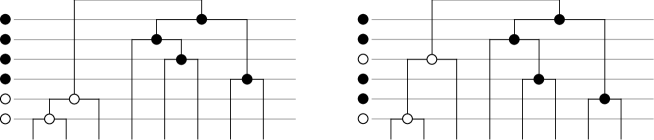
Figure 2: A shuffle at a given internal node. Bifurcations on the left subtree are marked with a hollow circle, and those on the right subtree are marked with a solid circle. The relative timing for these events is shown beside the tree; we call this sequence of symbols a “shuffle.” A set of shuffles for every internal node of a phylogenetic tree exactly determines the relative order of bifurcation events. Similar type symbols occurring together as in the left tree is evidence of lineage-specific bursts.

We now make more formal definitions of our terms. For the purposes of this paper, a phylogenetic tree is a rooted tree with distinct leaf labels. We will denote the set of interior nodes of a phylogenetic tree $T$ with $N_{T}$. For an internal node $v$ in $N_{T}$, define $T_{v}$ to be the rooted subtree of $T$ containing all the descendants of $v$. The “daughter trees” of $v$ are the two subtrees of $T_{v}$ which we obtain by deleting $v$ and its two incident edges. For the first part of the paper, we assume that the phylogenetic trees are bifurcating. We describe later how to generalize the ideas presented to the case of multifurcating trees. A rank function on an arbitrary set $S$ is simply an ordering of the elements of that set; mathematically it is a one-to-one mapping from $S$ to ranks $\{1,2,\ldots,|S|\}$. A rank function on a phylogenetic tree $T$ is a rank function on the set of interior vertices $N_{T}$ with the property that the ranks are increasing on any path from the root to a leaf. We call a phylogenetic tree with a rank function a ranked phylogenetic tree or simply ranked tree (Semple and Steel, 2003).

In mathematics, a total order on a set is simply a binary relation (usually written $<$) such that for any two distinct elements $a$ and $b$ of the set either $a<b$ or $b<a$. Note that a rank function on a set is equivalent to a total order on that set: given a total order one can rank the elements in increasing order of rank, and given a rank function one can define a total order by numerical inequality of rank. Thus a ranked phylogenetic tree is exactly a tree equipped with a total order on its internal nodes.

In this paper, an $(m,n)$ shuffle on symbols $p$ and $q$ is simply a sequence of length $m+n$ containing $m$ $p$’s and $n$ $q$’s. (The complete terminology for such a sequence is riffle shuffle (Aldous and Diaconis, 1986).) For example $pqppq$ is a $(3,2)$ shuffle on $p$ and $q$. The utility of these shuffles in the present context is summarized in the following observation.

Observation 1.

Given totally-ordered sets $P$ and $Q$, the total orderings of $P\cup Q$ respecting the given orderings of $P$ and $Q$ are in one-to-one correspondence with the $(|P|,|Q|)$ shuffles on symbols $p$ and $q$.

To see how this works, assume total orders $p_{1}<p_{2}<\cdots<p_{m}$ on $P$ and $q_{1}<q_{2}<\cdots<q_{n}$ on $Q$ are given, along with a $(m,n)$ shuffle on $p$ and $q$. The required total ordering on $P\cup Q$ is obtained by progressing along the shuffle and substituting $p_{i}$ and $q_{j}$ for $p$ and $q$ in order: for example the shuffle $pqppq$ uniquely defines the total order $p_{1}<q_{1}<p_{2}<p_{3}<q_{2}$ when $p_{1}<p_{2}<p_{3}$ and $q_{1}<q_{2}$. In the other direction, a total ordering on $P\cup Q$ uniquely defines a $(|P|,|Q|)$ shuffle and a total ordering on each of $P$ and $Q$.

We can use shuffles to develop a recursive formulation of ranked phylogenetic trees. Assume that $v$ is an internal node of a tree and that the tree $T_{v}$ containing the descendants of $v$ is composed of two daughter subtrees $L_{v}$ and $R_{v}$. Assume $L_{v}$ and $R_{v}$ have $m$ and $n$ internal nodes, respectively. We define a “shuffle at an internal node” $v$ to be a $(m,n)$ shuffle on symbols $\ell$ and $r$. Assume $L_{v}$ and $R_{v}$ are ranked subtrees, i.e. there is a total ordering on the internal nodes of each of $L_{v}$ and $R_{v}$. By Observation 1, a total ordering on the internal nodes of $T_{v}$ respecting the orderings on the internal nodes of $L_{v}$ and $R_{v}$ is equivalent to a shuffle at the internal node $v$. Therefore we can recursively reconstruct the rank function for any ranked tree given a shuffle at each internal node. We define a tree shuffle to be such a choice of shuffles. With Observation 1, we have the following result, which is crucial to our analysis:

Observation 2.

Each rank function on a given tree being equally likely is equivalent to the statement: For each internal node $v$, each shuffle at $v$ is equally likely.

Neutral models for ranked trees

In this section we formulate two classes of neutral models. First we introduce the constant across lineages models, which are an obvious generalization of the coalescent/Yule models. Then we introduce the constant relative probability models, which generalize coalescent/Yule models in a new direction. The common theme between these two classes of models is that they both induce the uniform distribution on shuffles.

Ranked oriented trees

In this section it will be convenient to discuss ranked oriented trees rather than ranked phylogenetic trees. This allows us to distinguish the children of each vertex without having to explicitly label species which may later become extinct. The distributions and statistics considered in this paper may be easily transferred between these two types of trees, as well as ranked unlabeled trees, which we call ranked tree shapes. For the present purposes, definitions and proof are much easier in the case of ranked oriented trees.

Definition 3.

A oriented tree is a finite rooted binary tree where the children of each internal node are labeled left and right respectively. A ranked oriented tree is a oriented tree with a rank function.

Note that here “tree” in this definition is not short for “phylogenetic tree.” That is, our notion of ranked oriented tree does not include leaf labels. These trees are called “oriented” because they are oriented graphs, i.e. the edges around each vertex have a fixed orientation.

There is a map from ranked oriented trees to ranked tree shapes which forgets the ordering of children. Similarly, there is a map from ranked phylogenetic trees (called ranked trees in this context) to ranked tree shapes which forgets leaf labels. Both of these “forgetful” maps induce maps between probability distributions on these sets of trees.

We now prove that the uniform distributions on ranked oriented trees and on ranked phylogenetic trees induce the same distribution on ranked tree shapes.

Recall that at cherry is a pair of adjacent leaves: two leaves with the same parent.

Proposition 4.

Given a ranked tree shape with $n$ leaves and $k$ cherries, there are $2^{n-1-k}$ ranked oriented trees sent to it by the forgetful map.

Proof.

First, note that the $n-1$ internal nodes of a given ranked tree shape are distinguished by their rank. Thus every ranked oriented tree which maps to this tree shape must be formed by assigning an orientation at each of these internal nodes. For each of these there are two possible left-right labelings of the child subtrees, giving $2^{n-1}$ ranked oriented trees. However, for the $k$ internal vertices which are the parents of a pair of leaves the ordering of children does not effect the resulting ranked oriented tree. For all other $n-1-k$ internal vertices the ranking of internal vertices ensures that the two orderings of child subtrees are distinguishable. Thus there are exactly $2^{n-1-k}$ distinct ranked oriented trees. ∎

Proposition 5.

Given a ranked tree shape with $n$ leaves and $k$ cherries, there are $\frac{n!}{2^{k}}$ ranked phylogentic trees sent to it by the forgetful map.

Proof.

Similarly to the previous proof, there are $n!$ ways to label the identified leaves of a ranked tree shape. However, the labels of the two leaves of a cherry may be switched without changing the ranked phylogentic tree. Such switches (and their combinations) are the only such transformations which leave the phylogenetic tree unchanged. Thus, there are $\frac{n!}{2^{k}}$ distinct leaf labelings of the ranked tree shape. ∎

Together, these give us the desired result:

Proposition 6.

A uniform distribution on ranked oriented trees with $n$ leaves and a uniform distribution on ranked phylogenetic trees with $n$ leaves both induce the same distribution on ranked tree shapes.

Proof.

Given a ranked tree shape with $n$ leaves and $k$ cherries, there are $2^{n-1-k}=2^{n-1}/2^{k}$ ranked oriented trees which map to this tree and $n!/2^{k}$ ranked phylogenetic trees which map to this tree. Thus, for both of the induced probabilities on ranked tree shapes, the ratio between the probability of a tree with $k$ cherries and the fixed tree with $1$ cherry is $1/2^{k-1}$. As both distributions are probabilities they must be equal. ∎

Proposition 7.

There are $(n-1)!$ ranked oriented trees on $n$ leaves.

Proof.

Proceed by induction on $n$; for $n=2$ the statement is obviously true. Suppose there are $(n-1)!$ ranked oriented trees (ROTs) with $n$ leaves. Now note that the next bifurcation event is uniquely identified by its rank, and it can occur in $n$ places, thus there will be $n!$ ROTs with $n+1$ leaves. ∎

It is well known that the Yule model gives the uniform distribution on ranked phylogenetic trees on $n$ taxa for each $n$ (Edwards, 1970). By Proposition 6, this corresponds to the uniform distribution on ranked oriented trees. A direct proof goes as follows:

Proposition 8.

The Yule model results in the uniform distribution on ranked oriented trees with $n$ leaves after $n-1$ bifurcations.

Proof.

Given a ranked oriented tree with $n$ leaves, there are $n$ possible places for a bifurcation event to occur. These are all equally likely. By induction the $(n-1)!$ ranked oriented trees with $n$ leaves were all equally likely, so the $n!$ ranked oriented trees with $n+1$ leaves are also all equally likely. ∎

The following lemma will be useful shortly.

Lemma 9.

Given a ranked oriented tree (ROT) with $n$ leaves, there are $n(n+1)$ ways to add an additional leaf.

Proof.

First, decide which rank the new internal node will have, from $1$ (earliest) to $n$ (latest). If the new internal node has rank $k$ then there are $k$ choices at that level for the edge to add it to, and then $2$ choices for which side of this edge the new pendant leaf will sit. This gives a total of $2\sum_{i=1}^{n}i=2\frac{n(n+1)}{2}=n(n+1)$ ways to insert the new leaf edge. ∎

In the sequel, we consider forward time ranked-oriented-tree-valued stochastic processes. In particular we consider birth-death processes where the transitions between trees involve either an bifurcation or deletion event (e.g. speciation or extinction). Call these ranked-oriented-tree birth-death processes. The details of bifurcation (birth) and extinction (death) events are as follows. If there is a bifurcation event, in which two pendant leaves are attached to an existing leaf, the new branches descending from the bifurcation event are assigned left and right. If there is an extinction event, occurring at a leaf vertex, the leaf and its adjacent edge are deleted. The ancestor of the extinct leaf is now a degree-two vertex. This vertex is suppressed by replacing it and its two adjacent edges by a single edge, with an orientation for the new edge inherited in the obvious way. In this way, the ancestor still has a left and right child. The ranking of internal vertices is induced by the time ordering of their associated bifurcation events. If extinction events do not occur then call such a process a pure-birth ranked-oriented-tree process.

In the later section on example applications we consider, for computational convenience, the likelihood of rank functions on tree shapes rather than on oriented trees. The following proposition and corollary show that the uniform distributions on rank functions of oriented trees in the models and analysis which follow induce uniform distributions on tree shapes when orientation is forgotten. In particular, $p$-values for such rank functions may be computed over either oriented or unoriented tree shapes.

First, define a symmetric vertex to be one for which the unoriented shapes of the subtree below each child of this vertex are the same (isomorphic as tree shapes). A big symmetric vertex is a symmetric vertex with more than two leaves below.

Proposition 10.

A uniform distribution on rank functions on a given oriented tree induces a uniform distribution on rank functions of its corresponding tree shape.

Proof.

Let $t$ be an oriented tree with $n$ leaves and $t^{\prime}$ its corresponding tree shape. Let $q$ denote the number of big symmetric vertices of $t$. For $n=2$, which implies $q=0$, we have for the ranking on $t^{\prime}$ exactly $1=2^{0}$ ranking on $t$. Assume the following statement is true for all oriented trees with less than $n$ leaves: for each ranking on $t^{\prime}$ there are exactly $2^{q}$ rankings on $t$ which are sent to it by the map which forgets orientation of vertices. The induction now breaks into three cases.

Case 1: Suppose the two children of the root branch-point of $t^{\prime}$ are non-isomorphic tree shapes, each having more than $1$ leaf. They may therefore be distinguished from each other, and given a ranking on $t^{\prime}$ the shuffle at the root node of $t$ is determined. Call the two child subtrees “left” and “right” with $q_{1}$ and $q_{2}$ big symmetric vertices, respectively. By the inductive assumption, there are $2^{q_{1}}$ rankings for the left subtree of $t$ and $2^{q_{2}}$ rankings for the right subtree which map to the corresponding rank function on the left and right subtree shapes. This gives $2^{q_{1}+q_{2}}$ total since there is no choice for the shuffle at the root branch-point of $t$. This is the number of big symmetric vertices of $t^{\prime}$.

Case 2: Suppose the two children of the root branch-point of $t^{\prime}$ are non-isomorphic tree shapes, one of the children being a leaf. They may therefore be distinguished from each other, and given a ranking on $t^{\prime}$ the shuffle at the root node of $t$ is determined. The bigger subtree $t_{b}$ has $q_{b}$ big symmetry vertices. By the inductive assumption, there are $2^{q_{b}}$ rankings for $t_{b}$ which map to the corresponding rank function on its shape. Attaching a leaf to $t_{b}$ to obtain $t$ does not change the number of rankings for $t$ or $t^{\prime}$. Therefore, there are $2^{q_{b}}$ rank functions on $t$ which map to the given rank function on $t^{\prime}$, and $q_{b}$ is the number of big symmetric vertices of $t^{\prime}$.

Case 3: Suppose that the two children of $t^{\prime}$ are isomorphic. Therefore they may not be distinguished except by the ranking. Therefore the shuffle at the root branch-point of $t$ is only determined up to swapping the left and right subtrees. After this choice the two subtrees are distinguished: which subtree of $t^{\prime}$ is “left” and which is “right” is determined by the shuffle. The rest of the argument proceeds as before, except that this time there are $2^{q_{1}+q_{2}+1}$ rank functions on $t$ which map to the given rank function on $t^{\prime}$, and $q_{1}+q_{2}+1$ is the number of big symmetric branch-point of $t^{\prime}$.

The result now follows by induction. ∎

Corollary 11.

If a probability function on ranked oriented trees is uniform on rank functions conditioned on oriented tree then it is also uniform on rank functions of an (unoriented) tree shape when conditioned on that (unoriented) tree shape.

Proof.

This follows from the previous proposition because the resulting mixture of uniform distributions on rank functions on $t^{\prime}$ (one for each oriented tree $t$ with shape $t^{\prime}$) is also uniform. ∎

This corollary allows us to apply our rank tests to trees which are given without orientation– ranked tree shapes.

Constant across lineages (CAL) models

We define a constant across lineages (CAL) model to be a forward time ranked-oriented-tree birth-death process such that any new (bifurcation or extinction) event is equally likely to occur in any extant lineage. You may also think of the projection of this process onto ranked trees, by forgetting the orientation of children at each internal vertex. Any model described in terms of rates is a CAL model if the bifurcation and extinction rates are equal between lineages at any given time. However, these rates may vary in an arbitrary fashion depending on time or the current state of the process. This class of models includes the Yule model (Yule, 1924), the critical branching process model (Aldous and Popovic, 2005), the constant rate birth and death process (Nee et al., 1994) and the coalescent (Kingman, 1982).

However, the CAL class is more general. It includes macroevolutionary models that have global speciation and extinction rate variation, for example due to global environmental conditions. Furthermore, it is also possible to incorporate models which take into account incomplete random taxon sampling, which is equivalent to the deletion of $k$ species uniformly at random from the complete tree. Indeed, if the complete tree evolved under a CAL model then we simply run the model for longer with the probability of bifurcation set to zero and the extinction probability non-zero (and uniform across taxa). This extended model is clearly still within the CAL class.

The CAL class also includes microevolutionary models such as the coalescent with arbitrary population size history. This very simple but important fact means that the tests for non-neutral diversification described in later sections are not fooled by ancestral population size variation (as are a number of other tests in the literature).

The CAL definition is a generalization of the “exchangeable” criterion from Aldous (2001), and we acknowledge the importance of Aldous’ ideas in formulating the definition.

Proposition 12.

At all times in a CAL model, the distribution of ranked oriented trees with $n$ leaves is uniform.

Proof.

Assume that after $k$ events, all $(m-1)!$ ranked oriented trees (ROTs) of size $m$ are equally likely. If the next event is a bifurcation then, because the result of each (tree, bifurcation event) pair is distinct, after this event all $m!$ ROTs with $m+1$ leaves are equally likely. Similarly, if the next event is an extinction then for each of the $(m-1)!$ equally likely trees there are $m$ equally likely choices for which leaf to extinguish, giving $m!$ possibilities in all. By Lemma 9 each ROT with $m-1$ leaves results from $m(m-1)$ of these tree-plus-leaf choices. Thus each ROT with $m-1$ leaves is equally likely, with probability $m(m-1)*1/m!=1/(m-2)!$.

Since this is true for any such sequence of bifurcations and extinctions it is true at all times. ∎

Recall that this corresponds to a uniform distribution on ranked phylogenetic trees, by Proposition 6.

Of course, any model giving the uniform distribution on ranked trees with $n$ tips gives the uniform distribution on rank assignments given a topology with $n$ tips. Thus

Corollary 13.

Any CAL model gives the uniform distribution on rank assignments (and thus tree shuffles) given a tree topology.

We have the following limited converse of Proposition 12.

Proposition 14.

Pure-birth CAL models are the precisely the set of pure-birth ranked-oriented-tree processes which, for any $n\geq 1$, give the uniform distribution on ranked oriented trees with $n$ taxa when halted as soon as $n$ taxa are present.

Proof.

By the proof of Proposition 12, pure-birth CAL models result in a uniform distribution on ranked oriented trees of size $n$ (since there have been exactly $n-1$ events).

Now consider a model which does not satisfy the CAL condition. Assume that the $k$-th bifurcation event was not picked uniformly among lineages, i.e. there is a ranked tree $T_{0}$ with lineages $l_{1}$ and $l_{2}$ which have probabilities $p_{1}\neq p_{2}$ to speciate. Let $T_{1}$ (respectively $T_{2}$) be the ranked tree produced if $l_{1}$ (respectively $l_{2}$) bifurcates. In a pure birth process, $T_{1}$ and $T_{2}$ may only be reached in this way. Now

$${\mathbb{P}}[T_{1}]={\mathbb{P}}[T_{0}]\cdot p_{1}\neq{\mathbb{P}}[T_{0}]\cdot p_{2}={\mathbb{P}}[T_{2}]$$

which shows that this model cannot give the uniform distribution on ranked trees when the process is halted at $k$ taxa. There is only one way to build each ranked oriented tree with $n$ leaves so the distribution on these cannot be uniform, since an equal number must descend from each of $T_{1}$ and $T_{2}$. Thus, by contradiction, there is no such $k$ and so no such model. ∎

Note that in the last proposition, the restriction to a pure-birth process is needed. Consider a process with extinction where bifurcation is equally likely for each species but extinction is history dependent: whenever an extinction event occurs, it undoes the most recent bifurcation event. This model clearly does not belong to the class of CAL models. However, it gives a uniform distribution on ranked trees of some fixed size.

Constant relative probability (CRP) models

The motivation for the constant relative probability (CRP) models comes from considering the models on ranked trees which might emerge from non-selective diversification, perhaps based on physical or reproductive barriers. For example, assume we could watch a set of species emerge via allopatric speciation, and the fundamental geographic barrier is a mountain range dividing land into two regions, $A$ and $B$. These regions may differ in size or fecundity, so there may be some difference in the rate of diversification in $A$ versus $B$. However, our neutral assumption for the CRP class is that the relative rate stays constant over time. In contrast, non-neutral models might dictate that a bifurcation in one region will shift the equilibrium such that further diversification in that region will become more likely (“bursting” diversification) or less likely (“refractory” diversification).

Again, for convenience, we work with ranked oriented trees so we may distinguish the two children of any bifurcation event. For each internal node, $v$, (representing a bifurcation event) let $L_{v}$ and $R_{v}$ denote the “left” and “right” lineages descending from $v$ (daughter subtrees of $v$).

A constant relative probability (CRP) model is a forward time pure-birth ranked-oriented-tree process together with a probability distribution $P$ on the unit interval $[0,1]$, where each internal vertex has a real number, $p_{v}$ associated with it. Each new bifurcation occurring in the clade below $v$ occurs in $L_{v}$ with probability $p_{v}$, and occurs in $R_{v}$ with probability $1-p_{v}$. For each new bifurcation event (internal vertex), $v$, choose the value $p_{v}$ by an independent draw from $P$. As with CAL models, there is no constraint of any kind on waiting times between bifurcation events.

Recall the map from ranked oriented trees to unranked oriented trees which forgets the rank ordering of internal nodes and the leaf labels. The image of a ranked tree under this map is its oriented tree. Similarly, if the orientation is also forgotten then call the image the tree shape of the initial tree.

Proposition 15.

A CRP model, stopped at a time depending only on the time and number of leaves, gives the uniform distribution on rank functions for each oriented tree.

Proof.

Consider the distribution of ranked oriented trees resulting from the stopped CRP. Consider a particular oriented tree, $t$, with $k$ internal vertices $v_{1},\ldots,v_{k}$. Let $n_{i}$ and $m_{i}$ denote the number of internal vertices below the left and right subtrees, respectively, of vertex $v_{i}$. Fix a ranking on this tree. We now compute the probability of this ranked oriented tree under the model (conditional on the total number of leaves). Fix an assignment of $p_{v_{i}}$ to each internal vertex $v_{i}$. Given this choice, the probability of the given ranked tree is the product of the probabilities of each bifurcation event. For a bifurcation at vertex $v_{i}$, the probability of this event is the product of $p_{v_{j}}$ for all $v_{j}$ for which $v_{i}$ lies on its left subtree times the product of $(1-p_{v_{j}})$ for all $v_{j}$ for which $v_{i}$ lies on its right subtree. In the product of these probabilities over all $v_{i}$, the term $p_{v_{j}}$ occurs exactly $n_{j}$ times (once for each internal vertex on the left subtree of $v_{j}$) and the term $(1-p_{v_{j}})$ occurs exactly $m_{j}$ times (once for each internal vertex on the right subtree of $v_{j}$). Thus, the probability of this ranked tree (given the choice of $p_{v}$) is:

$$\prod_{j=1}^{k}p_{v_{j}}^{n_{j}}(1-p_{v_{j}})^{m_{j}}$$

Note that this is independent of the ranking. Since the $p_{v_{i}}$ are picked independently from a distribution $P$, the probability of this ranked tree shape is

$$\int_{p_{v_{1}}}\cdots\int_{p_{v_{k}}}\prod_{j=1}^{k}p_{v_{j}}^{n_{j}}(1-p_{v_{j}})^{m_{j}}dP\cdots dP$$

which is again independent of the ranking. Therefore, all rankings of this oriented tree are equally likely. ∎

Note that the CRP generalizes the stick-breaking models (Aldous, 1995). Recall that with the stick-breaking model, a stick is recursively broken into pieces, with the break point of each piece chosen independently from a probability $P$ on the open unit interval $(0,1)$. For example, if the number chosen for a piece was $1/2$ then that piece is broken into two equal sized pieces. For each piece a new draw is taken from $P$ to determine the how far along to break it. To generate a finite oriented binary tree with $n$ leaves, first break a stick as just described then choose $n$ points from the unit interval uniformly at random. This determines a consistent set of partitions corresponding to a binary tree.

It is well known that the Yule model is generated by setting $P$ to the uniform measure on $(0,1)$. Similarly, Aldous’s Beta model corresponds to setting $P$ to be a beta measure.

Thus, the CRP process produces oriented ranked versions of such trees in a sequential growth process.

Tests for bursting diversification based on shuffles

In the previous section, we demonstrated that any model satisfying the constant across lineages or constant relative probability criteria induces the uniform distribution on tree shuffles. In this section we describe a way of testing for deviation from the uniform distribution on tree shuffles, and thus test for deviation from these neutral models. We emphasize that this can go significantly beyond testing the coalescent/Yule model, which is typically considered to be the definition of neutrality. Indeed, rejection of the uniform distribution on shuffles rejects all of the CAL and CRP models simultaneously, and the coalescent/Yule model is only one model in these classes. We note further that although the focus of this section is to consider all of the shuffles of a ranked tree at once, one can also consider a shuffle at a particular node as described in the introduction.

There are several useful tools available to test whether a shuffle is likely to have come from the uniform distribution on shuffles. In fact, a number of tests in the statistics literature have been developed for testing equality of distributions which actually implement a test of deviation from the uniform distribution for shuffles. These tests work as follows: assume we are given two sets of samples $\{\ell_{i}\}_{i=1,\ldots,m}$ and $\{r_{j}\}_{j=1,\ldots,n}$ and would like to test the hypothesis that they are draws from the same distribution. To test, combine the draws and put the samples in increasing order (assume that all draws are distinct). This clearly gives a shuffle on symbols $\ell$ and $r$. If the draws are from identical distributions then the induced distribution on shuffles will be uniform; if on the other hand symbols cluster together in the shuffle, there is some evidence that the draws are from unequal distributions.

One can then test deviation from the uniform distribution on shuffles in one of several ways. One way is to count the number of “runs.” As described in the introduction, a run is simply a sequence within the shuffle using only one symbol; the shuffle $\ell\ell rrrr\ell$  has three runs. Let $X_{m,n}$ denote the number of runs under the uniform distribution on shuffles on $m$ symbols of one type and $n$ of another. The distribution of $X_{m,n}$ is classical (see, e.g. Hogg and Craig (1994)):

$$\begin{split}{\mathbb{P}}\{X_{m,n}=2k+1\}&=\frac{{m-1\choose k}{n-1\choose k-1}+{m-1\choose k-1}{n-1\choose k}}{{m+n\choose m}}\\ {\mathbb{P}}\{X_{m,n}=2k\}&=\frac{2{m-1\choose k-1}{n-1\choose k-1}}{{m+n\choose m}}.\end{split}$$ (1)

Asymptotic results for the mean and variance are also known:

$${\mathbb{E}}[X_{m,n}]=\mu_{m,n}=2\frac{mn}{m+n}+1,\qquad{\rm Var}[X_{m,n}]=\frac{(\mu_{m,n}-1)(\mu_{m,n}-2)}{m+n-1}.$$

The usual application of the runs test makes a shuffle from the two draws as described above, calculates the number of runs in the shuffle, and then uses the above-calculated probabilities to test deviation from the uniform distribution on shuffles. However, the same method can be applied in any situation to test deviation from the uniform distribution on shuffles. In the present case, we can use an analogous process to investigate tree shuffles.

As described in the introduction, a tree shuffle simply assigns a shuffle of appropriate size to each internal node of the tree; from the previous section we expect these shuffles to be distributed uniformly for a variety of neutral models. Using runs we can test whether a single shuffle is drawn from the uniform distribution, but some method is needed to combine this information across the internal nodes of the tree.

We chose to combine our data from each vertex by simply summing the number of runs across all of the shuffles in the corresponding tree shuffle. Let ${\mathcal{R}}(T)$ denote this number. The distribution of ${\mathcal{R}}(T)$ (under the assumption that each shuffle is equally likely) can be calculated recursively as shown in the next several paragraphs. There are two cases to consider. First, one may condition on the observed tree topology and calculate the neutral distribution of ${\mathcal{R}}(T)$ in that setting. A second option is to test deviation from a neutral model which gives the uniform distribution on ranked trees. This is a stronger statement than saying that a given model induces the uniform distribution on shuffles conditioned on the phylogenetic tree.

We first condition on the observed tree. Uniform shuffles conditioned on the tree shape are obtained in the CRP and the CAL class of models. For a tree with one leaf, we have ${\mathbb{P}}\{{\mathcal{R}}(T)=0\}=1$. For a tree with two leaves, we also have ${\mathbb{P}}\{{\mathcal{R}}(T)=0\}=1$ (the two daughter subtrees have no internal nodes).

For a tree $T$ with uniform random ranking, composed of two ranked subtrees $L$ and $R$ of size $m$ and $n$, respectively, we have:

$${\mathbb{P}}\{{\mathcal{R}}(T)=k\}=\sum_{i=0}^{k}{\mathbb{P}}\{X_{m,n}=i\}\sum_{j=0}^{k-i}\ {\mathbb{P}}\{{\mathcal{R}}(L)=j\}{\mathbb{P}}\{{\mathcal{R}}(R)=k-i-j\}.$$ (2)

It is shown in the Appendix that this distribution can be calculated on a tree with $n$ leaves in time $O(n^{3}\log^{2}n)$. Thus it is practical to obtain a $p$-value for ${\mathcal{R}}(T)$ analytically.

Now we take the second approach, assuming we want to test a model such that each ranked tree is equally likely. This includes the CAL models, and in the case of pure birth models, this is exactly the set of the CAL models (Proposition 14). Let ${\mathcal{R}}(n)$ be the random variable “runs of a tree with $n$ leaves” where the tree is drawn from the uniform distribution on ranked trees. The distribution of ${\mathcal{R}}(n)$ can again be obtained recursively. Note that for a uniform ranked tree on $n$ leaves, the probability that one daughter tree has size $r$ and the other daughter tree has size $n-r$ is $1/(n-1)$ for all $r$. Thus

$$\begin{split}{\mathbb{P}}\{{\mathcal{R}}(n)=k\}=\frac{1}{n-1}\sum_{r=1}^{n-1}\sum_{i=1}^{k}&{\mathbb{P}}\{X_{r,n-r}=i\}\times\\ &\sum_{j=0}^{k-i}\ {\mathbb{P}}\{{\mathcal{R}}(r)=j\}{\mathbb{P}}\{{\mathcal{R}}(n-r)=k-i-j\}.\end{split}$$ (3)

The complexity for recursively calculating the distribution of runs for trees with $n$ leaves is $O(n^{4}\log^{2}n)$, by an argument analogous to that for Equation (2).

Note that there are a number of alternative ways to “sums of runs” for testing deviation from the uniform distribution on shuffles. First, we have made one choice— namely, summation— concerning how the statistics for each shuffle are combined. One certainly could use an alternative method, potentially including weights. Second, there are other statistics such as Mann-Whitney-Wilcoxon which could be used in place of the runs statistic. The advantage of summation is that it results in simple formulas, and the advantage of the runs statistic is that it is easy to interpret. We have not tested any alternate formulations.

A python package for computing quantiles of shuffles is available at

http://www-m9.ma.tum.de/twiki/bin/view/Allgemeines/TanjaGernhard

One of the main features of this package is the ability to calculate the quantile of the runs statistic assuming a uniform distribution on rankings for a set of input trees. The quantiles can be calculated conditioned on a given tree shape, or under the assumption of a uniform distribution on ranked trees. For a collection of trees (e.g. a sample from the Bayesian posterior), the individual quantiles can be averaged. In addition to the calculation of the runs statistic and the quantile for the whole tree, the package can calculate the runs statistic and quantile for each interior vertex of a single tree. This feature may be useful for biologists looking for signals of a key innovation.

Shuffles in the Bayesian setting

In our work up to now, we have assumed that the correct tree and diversification timing information is known. This assumption is not realistic for a number of datasets. For example, below we apply our methodology to a sample of Hepatitis C viruses, which probably do not have enough sequence divergence to perfectly reconstruct a phylogenetic tree with timing information.

One way of working with such datasets is to take a Bayesian approach, where rather than a single tree one gets a posterior distribution on trees. For each single tree, one can compute the quantile of the total runs statistic, either conditioning on the topology or assuming a Yule distribution of ranked tree shapes. We then simply take the average of the quantiles thus computed for each tree. Such averaging can be justified in a manner similar to the work of Drummond and Suchard (2007), except that no further simulation is needed to compute the $p$-value. The average of $p$-values in this case is not exactly uniformly distributed under the neutral model as a proper $p$-value should be, although the averaged distribution does share many of the characteristics of a classical $p$-value (Meng, 1994).

Runs and neutrality

Here we note that the runs statistic can be used to test the coalescent in the presence of ancestral population size variation. Tests of neutrality in the presence of historical population size variation are of particular recent importance, as new coalescent-based methods are in use to infer population size history in a Bayesian framework (Drummond et al., 2005; Opgen-Rhein et al., 2005). If these methods are to be used on a given set of sequences it is important to test the central assumption of the methods, namely that the sequences have a genealogy which can be accurately described using the coalescent with arbitrary population size history.

Unfortunately, classical statistics such as the $D$ statistics of Tajima (1989) and Fu and Li (1993) confound ancestral population size changes and non-neutral evolution. One solution to this problem is to investigate the Bayesian posterior on phylogenetic trees for evidence of non-neutral evolution rather than using the sequence information directly. This has been done by Drummond and Suchard (2007), who use a posterior predictive $p$-value approach. Here we simply point out that, as described above, the coalescent with arbitrary population size history is a CAL model and thus will induce the uniform distribution on ranked phylogenetic trees; thus by rejecting the CAL class we reject a general coalescent model. We will apply this fact below in the example application to Hepatitis C data.

Generalization for non-binary trees

Polytomies (i.e. non-binary splits) are common in reconstructed phylogenetic trees. Some polytomies are certainly due to a lack of information to resolve the splits, however it has been argued that molecular and species level polytomies actually exist (Jackman et al., 1999; Slowinski, 2001). The methodology described in this paper can be extended to trees with “hard” polytomies, i.e. cases of multiple divergence which are essentially simultaneous in evolutionary time.

The new ingredient needed is the “multiple runs distribution,” i.e. the analog of (1) for shuffles on more than two symbols. This is described in David and Barton (1962). Using these distributions, the probability of a shuffle consisting of symbols from the $k$ daughter trees can be found for a shuffle at a non-bifurcating split $v$.

Example applications

In this section we describe two distinct applications of the methods in this paper. First, we apply the methods to E1 gene data for the Hepatitis C virus (HCV). This data set shows some limited– though consistent– lineage-specific bursting diversification, showing that neither CAL nor CRP models accurately describe the sort of evolution observed. However, an analysis not conditioning on tree shape clearly rejects any CAL model, such as the coalescent with varying population size. The second application is to phylogenetic trees for ants, whose timing information was reconstructed through fossils and the r8s (Sanderson, 2003) rates smoothing program. These ant trees do not show any evidence of lineage-specific bursting evolution, despite some interesting history in terms of diversification rates.

Our HCV data comes from two independent studies: one in China (Lu et al., 2005), and one in Egypt (Ray et al., 2000). The HCV alignments were retrieved from the LANL HCV database (Kuiken et al., 2005) via PubMed article ID numbers. The Chinese dataset contained samples from 132 infected individuals, and the Egyptian dataset had samples from 71 individuals. We randomly partitioned the taxa from the Chinese dataset into three sets of 44 taxa each and used the corresponding sub-alignments as distinct data sets. The Egyptian data was similarly split into two sub-alignments of size 37 and 36. This partitioning was done in order to have a larger number of similar datasets from which we could investigate the dynamics of HCV evolution, and to demonstrate that non-neutral evolution can be seen even with an moderate number of taxa.

In order to avoid confounding temporal information with molecular rate variation, we applied the relaxed clock model of Drummond et al. (2006b) as implemented in the BEASTv1.4 suite of computer programs (Drummond and Rambaut, 2007). We chose uncorrelated lognormally distributed local clocks, the HKY model, and four categories of gamma rate parameters in the gamma + invariant sites model of sequence evolution. We used both the constant population size and exponential growth coalescent priors. All other parameters were left as default; the corresponding BEAST XML input files are available from the authors upon request.

In each case the MCMC chain was run for 10 million generations, and convergence to stationarity checked with the BEAST program Tracer. For each model parameter, the minimum effective sample size (ESS) was at least 164, with most being significantly greater. The coefficient of variation of the relaxed clocks in the analysis had a minimum of 0.336 and an average of 0.491, indicating a significant deviation from a strict clock for this data set. The first 10% of the run was removed and 100 trees were taken from the tree log file, equally spaced along the run of the MCMC chain. We interpret these trees as being independent samples from the posterior. As a check, the analysis was run with an empty alignment and no consistent deviation from the uniform distribution on shuffles was detected (results not shown).

Data set	Const. cond.	Exp. cond.	Const. CAL	Exp. CAL
China set 1	0.232	0.254	0.0415	0.0601
China set 2	0.191	0.17	0.041	0.0349
China set 3	0.239	0.259	0.0287	0.0265
Egypt set 1	0.261	0.299	0.045	0.0624
Egypt set 2	0.308	0.256	0.0242	0.0188

Table 1: Expected quantiles of the number of runs in the posterior for a Bayesian analysis as described in the text. Each row represents one dataset. “Const.” means the BEAST analysis with a constant population coalescent prior, and “Exp.” denotes analysis an exponentially increasing population size coalescent prior. The “cond.” label means that we analyze conditional on tree topology, which gives us thus the quantile for any neutral model inducing the uniform distribution on shuffles. “CAL” denotes the runs quantile under the assumption of the uniform distribution on ranked trees, as would be the case for any CAL model, such as the coalescent with arbitrary population size history. As described in the text, the “cond.” columns show that some limited lineage-specific bursting is seen, and the CAL column rejects the coalescent with arbitrary population size history.

We have displayed the results in Table 1. In the columns labeled “cond.” we show the quantile of the number of runs conditioning on tree shape, calculated as in Equation (2). As can be seen, the results are substantially below one half, with the maximum being 0.308. Although this is not exceptionally strong lineage-specific bursting behavior, it does so consistently across five samples from two independent studies. Thus we feel confident in saying that the evolution of HCV displays lineage-specific bursting behavior. It might also be noted that these results were gained despite the fact that the coalescent was used as a prior. That is, if any bias could be expected in the Bayesian analysis, it would be towards a coalescent prior and a uniform distribution on shuffles, thus we believe our results form an upper bound for the actual statistics of the HCV lineages.

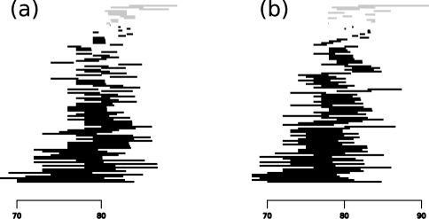
Figure 3: A visualization of the number of runs in a posterior sample of trees for an alignment of Hepatitis C sequence data of Ray et al. (2000). Black bars represent fewer runs than neutral, and gray the opposite. As described in the text, the width of the bars represents the amount of divergence from a broad class of neutral models. Said simply, each black bar represents a tree in the posterior which displays evidence of lineage-specific bursting diversification, and the longer the bar, the more bursting the tree. The bars are sorted vertically by increasing size (with sign.) Figure (a) shows the results when the tree prior in BEAST was taken to be coalescent with constant population size. Figure (b) shows the corresponding results with the exponentially increasing population size prior.

We have displayed a graphical representation of the results for the second Chinese data set in Figure 3. Each horizontal bar represents one of the 100 ranked trees from the posterior. One side of the bar gives the number of runs in the ranked tree $T$, and the other side gives the expected number of runs for a neutral (i.e. CAL or CRP) tree of the same unranked topology as $T$. If $T$ has more runs than the expectation, the bar is colored gray; if fewer it is colored black. In both the cases of constant population size and exponentially increasing population size coalescent prior for BEAST, it can be seen that there are fewer runs than the expectation, meaning that it appears that the HCV data under investigation may have had periodic bursts of diversification in its past.

Now we apply our techniques as a statistical test for the coalescent with ancestral population size variation as described above. This is topical: we note that the Ray et al. (2000) HCV data was analyzed by Opgen-Rhein et al. (2005) as an example application of a reversible-jump Bayesian MCMC algorithm for estimating demographic history of the virus. In doing so they made an implicit assumption of neutrality because their method [and other such methods (Drummond et al., 2005)] are based on the coalescent. They did not test this neutrality assumption as no methods were available at the time to test for neutral evolution in the presence of ancestral population size changes.

Our method can do so. Specifically, we compare the number of runs to the distribution for an arbitrary CAL model, as in Equation (3). By the results in the right half of Table 1, one can see that the data does not follow a coalescent model with arbitrary population size history. This implies a significant model mis-specification in the Opgen-Rhein et al. (2005) paper; it would be interesting to know how this would impact the historical population size estimates in their paper.

For the second application we investigated two different trees of ant taxa. The first tree is that of Moreau et al. (2006), showing the diversification of the major ant lineages. The timing information in this tree is quite remarkable, in that the corresponding lineages-through-time (LTT) plot shows a substantial increase in diversification rate during the Late Cretaceous to Early Eocene, which corresponds to the rise of angiosperms (flowering plants). Given the tools at our disposal, one might wonder if this increase in diversification rates affected all lineages equally, or if it occurred in lineage-specific bursts. The second ant tree we investigated was that of Pheidole, a “hyperdiverse” ant genus. Pheidole is almost certainly monophyletic, and yet comprises about 9.5% of the ant species in the world, according to latest estimates (Moreau, in review). Moreau has recently reconstructed a phylogeny of this genus which we have analyzed along with the tree of the ant lineages in general. Both trees were reconstructed via maximum likelihood, then made ultrametric using the penalized likelihood method of the r8s rates smoothing program (Sanderson, 2003).

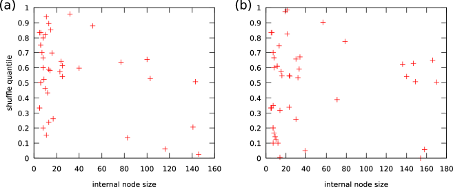
Figure 4: The distribution of the runs statistic for the internal nodes in two trees of ant taxa. Each point in each plot represents an internal node in the corresponding tree; the $x$ axis gives the number of taxa below the internal node and the $y$ axis gives the quantile of that internal node in terms of the runs statistic. Figure (a) is the tree of Moreau et al. (2006), and Figure (b) is a tree of Pheidole. These two trees do not appear to consistently show either lineage-specific bursting or refractory diversification.

In Figure 4 we show a plot of the internal nodes of each tree. The $x$ coordinate in the plot is the number of taxa below an internal node, and the $y$ axis is the quantile of the number of runs in the shuffle statistic. As can be seen, there is no clear correlation between number of taxa below an internal node and the shuffle statistic, and at no stage does diversification appear to be consistently bursting or refractory in a lineage-specific sense. We can also compute the quantile of the total number of runs across the tree: for tree (a) this is about 0.9052 and for tree (b) this is about 0.6718. Thus for these two ant trees we do not see any significant evidence of lineage-specific bursting or refractory diversification. This analysis forms an interesting counterpoint to the LTT results for the ants, which shows an overall increase in diversification in rate during the Late Cretaceous to Early Eocene across the entire tree.

Conclusion

We have developed a framework which allows testing for non-neutral diversification timing. Our work consists of three main components: first, a simple, recursive way of quantifying the relative timing information on a phylogenetic tree; second, two classes of neutral models on trees with timing information; and third, a summary statistic which allows comparison of reconstructed trees to these neutral models. In our methodology, timing information is considered relative to sister taxa and considered in the context of the tree, which may make it a valuable complimentary method to lineages-through-time plots. We compute the significance of the deviation of timing information from a neutral model analytically, using a simple method drawn from classical statistics.

This method was conceived for the macroevolutionary case, in order to find historical evolutionary patterns requiring explanation. However, it is also quite applicable in the microevolutionary case, where it can test neutrality in the presence of historical population size variation. This is particularly relevant as methods are becoming available to describe historical population size under a coalescent assumption.

We emphasize that our methodology can go substantially beyond testing for deviation from the constant rate birth and death models, which are usually the entire class of “neutral” models considered. Indeed, because any CAL or CRP model induces the uniform distribution on shuffles, deviation from this distribution is evidence to reject any model in the CAL or CRP classes. Such a conclusion is much stronger than deviation from a constant rate birth and death model, which is only one of the CAL models.

However, sometimes one may wish to test only a more restricted set of models, such as only the CAL models (which include the coalescent with arbitrary population size history) and not the more general CRP models. By testing a more restricted class of models, a particular dataset will be more likely to fall outside the chosen class. For example, in the application of our methods to Hepatitis C data above, the data consistently shows evidence of not coming from a CRP model, although the corresponding quantile is in the 0.17 to 0.31 range. However, if one tests for conformity to the CAL class (again, including the coalescent with arbitrary population size history) one obtains rejection at the 5% level.

We applied the methods on two types of data. First we investigated data for the Hepatitis C virus, demonstrating that it consistently shows evidence of some limited lineage-specific bursting evolution. We then applied our methods to reject the coalescent with arbitrary population size history for this data. Next, we investigated two phylogenetic trees of ants, which showed no evidence of unusual relative diversification rates, despite an interesting history of overall diversification rates.

We recall that our method uses “relative” timing information rather than actual branch lengths. In many ways this is an advantage. In a microevolutionary setting this means that the corresponding tests are invariant to changes in ancestral population size, and thus our test for neutrality is not “fooled” by ancestral population size variation. In a macroevolutionary setting the statistics are robust to branch length estimation error over long time scales. Such estimations are known to be difficult (Kimura, 1981). We note further that from a modeling perspective it is possible to specify a probability distribution on ranked phylogenetic trees without specifying a particular distribution on branch lengths. This flexibility means that it may be possible to reject many models at once as described above.

Nevertheless it may be useful at some future stage to combine topology and continuous branch length information, rather than the discretized version considered here. However, quantifying the shape of such objects appears to be challenging, as the relevant geometry is quite intricate (Billera et al., 2001; Moulton and Steel, 2004). In contrast, by discretization to ranked trees we obtain a purely combinatorial object.

We close by noting that although various techniques for reconstructing phylogenetic trees with timing information have been present for many years, these methods are currently seeing an intense period of development and will only improve. With this improvement we expect to see an increase in the number of trees present in the literature with interesting patterns of diversification timing due to adaptive radiation or other factors. We hope that our technique will prove to be a useful analytical tool for these future investigations, not only for finding interesting diversification patterns, but also for testing potential biases of timing reconstruction methods.

Acknowledgements

The idea of using ranked trees in this context was suggested by John Wakeley. The authors would like to thank Alexei Drummond, Arne Mooers, Allen Rodrigo, and Dennis Wong for helpful discussions. Mike Steel made several important suggestions, including the recursive calculation of $p$-values for the shuffles. Alexei Drummond gave very valuable advice on running BEAST. John Huelsenbeck generously allowed us to run BEAST on his cluster. Corrie S. Moreau supplied trees for analysis, and gave many very helpful comments on the manuscript. TG is funded by a PhD scholarship of the Deutsche Forschungsgemeinschaft. FAM is funded by the Miller Institute for Basic Research in Science at the University of California, Berkeley.

Appendix

Here we provide a proof of the time-complexity bound for the computation of the runs distribution ${\mathcal{R}}(T)$ (i.e. conditioning on a given tree shape). This distribution may be computed easily for certain tree shapes, such as the comb tree. However, here we provide a bound which holds for all tree shapes. This bound makes use of a bound on the number of runs in a ranked tree.

Let $r(n)$ denote the maximum number of runs for a ranked tree with $n$ leaves. Thus $r(1)=r(2)=0$, $r(3)=1$ and $r(4)=2$. Let $I_{i=n/2}$ be $1$ if $i=n/2$ and $0$ otherwise. For a tree with at least $2$ leaves, if the first branch point has $i$ leaves on one side and $n-i$ leaves on the other, with $i\leq n-i$, then the number of runs at this vertex may be up to $2(i-1)+1-I_{i=n/2}$ (note that we have an $(i-1,n-i-1)$ shuffle at this vertex). This maximum is obtained by a shuffle which interleaves the elements from each set, one from each side for as long as possible, starting with the largest side.

Thus, $r(n)$ satisfies the following recurrence: $r(1)=r(2)=0$ and for $n\geq 2$:

$$r(n)=\max_{1\leq i\leq n/2}\left(2i-1-I_{i=n/2}+r(i)+r(n-i)\right)$$

Proposition 16.

For all integers $n\geq 1$, $r(n)\leq n\log_{2}n$.

Proof.

The statement is true for $n=1$. Suppose that the statement is true for all $k<n$. Then,

$$r(n) = \max_{1\leq i\leq n/2}\left(2i-1-I_{i=n/2}+r(i)+r(n-i)\right)$$

$$\leq \max_{1\leq i\leq n/2}\left(2i-1+i\log_{2}i+(n-i)\log_{2}(n-i)\right).$$

Note that $2i-1$, $i\log_{2}i$ and $(n-i)\log_{2}(n-i)$ are all convex functions of $i$ so their sum is convex also. Thus, the maximum of $2i-1+i\log_{2}i+(n-i)\log_{2}(n-i)$ occurs at an extreme value. Setting $i=1$ gives $1+0+(n-1)\log_{2}(n-1)$, while setting $i=\frac{n}{2}$ gives $2\frac{n}{2}-1+2\frac{n}{2}\log_{2}\frac{n}{2}=n(\log_{2}2+\log_{2}\frac{n}{2})-1=n\log_{2}n-1$. Both of these values are less than $n\log_{2}n$ and so $r(n)$ must be at most $n\log_{2}n$. The result follows for all $n\geq 1$ by induction. ∎

We now proceed to bound the complexity of computing the distribution of runs for a tree. For a tree $T$ with $1$ or $2$ leaves, the number of runs is always $0$.

Let $T$ be a tree with $n\geq 3$ leaves; we assume a uniform distribution on tree shuffles. Let $L$ and $R$ be the two randomly ranked subtrees of $T$, with $a$ and $b$ leaves respectively.

Equation (2) may be rewritten as follows:

$${\mathbb{P}}\{{\mathcal{R}}(T)=k\} = \sum_{i=0}^{A_{1}}{\mathbb{P}}\{X_{a,b}=i\}\sum_{j=0}^{A_{2}}\ {\mathbb{P}}\{{\mathcal{R}}(L)=j\}{\mathbb{P}}\{{\mathcal{R}}(R)=k-i-j\}$$ (4)

$$= \sum_{i=1}^{A_{1}}{\mathbb{P}}\{X_{a,b}=i\}{\mathbb{P}}\{{\mathcal{R}}(L)+{\mathcal{R}}(R)=k-i\}$$

where $A_{1}=\min(k,n)$ and $A_{2}=\min(k-i,r(a))$. Note that $a+b=n\geq 3$ implies $X_{a,b}\geq 1$ and ${\mathcal{R}}(T)\geq 1$.

Since ${\mathcal{R}}(T)$ is supported on (i.e. zero outside of) $k=1,\ldots,\lfloor n\log_{2}n\rfloor$, and for each $k$, the computation of Equation (4) costs $2n-1$ operations, the cost of computing its distribution with this formula is at most $(\lfloor n\log_{2}n\rfloor)(2n-1)$ arithmetic operations plus the cost of computing ${\mathbb{P}}\{X_{a,b}=i\}$ for $i=1,\ldots,n$ and ${\mathbb{P}}\{{\mathcal{R}}(L)+{\mathcal{R}}(R)=x\}$ for $x=0,\ldots,r(n)-1\leq n\log_{2}n-1$.

For these fixed $a$ and $b$, the values of ${\mathbb{P}}\{X_{a,b}=i\}$ can be calculated using Equation (1) in constant time (at most $5*2+4=14$ arithmetic operations each) with a linear overhead as follows. The binomial coefficients ${a\choose k}$ for $a\leq b$ and $k\leq b$ in Equation (1) may be calculated with at most two arithmetic operations from the factorials, $j!$ for $1\leq j\leq n$, which may in turn be pre-calculated in linear time ($n-1$ multiplications). Thus, calculating ${\mathbb{P}}\{X_{a,b}=i\}$ for $i=1,\ldots,n$ takes at most $14n$ arithmetic operations, with a one-time overhead of $n-1$.

The distribution of ${\mathbb{P}}\{{\mathcal{R}}(L)+{\mathcal{R}}(R)=x\}$ is supported on $x=0,\ldots,\lfloor n\log_{2}n\rfloor-1$. It may be computed by repeated application of the formula

$${\mathbb{P}}\{{\mathcal{R}}(L)+{\mathcal{R}}(R)=x\}=\sum_{j=0}^{\lfloor(n-1)\log_{2}(n-1)\rfloor}{\mathbb{P}}\{{\mathcal{R}}(L)=j\}{\mathbb{P}}\{{\mathcal{R}}(R)=x-j\}$$

as long as the distributions of ${\mathcal{R}}(L)$ and ${\mathcal{R}}(R)$ are know. This computation requires at most $n\log_{2}n\left(2(n-1)\log_{2}(n-1)+1\right)$ arithmetic operations: at most $(n-1)\log_{2}(n-1)+1$ multiplications and $(n-1)\log_{2}(n-1)$ additions for each of $n\log_{2}n$ values of $x$. Note that the distribution of ${\mathbb{P}}\{{\mathcal{R}}(L)\}$ is supported by $j=0,\ldots,{\lfloor(n-1)\log_{2}(n-1)\rfloor}$, since $L$ has at most $n-1$ leaves.

So, if the distribution of ${\mathcal{R}}(L)$ and ${\mathcal{R}}(R)$ are known, the distribution of ${\mathcal{R}}(T)$ may be calculated in at most

$$(\lfloor n\log_{2}n\rfloor)(2n-1)+14n+n\log_{2}n\left(2(n-1)\log_{2}(n-1)+1\right)$$

arithmetic operations. This is at most

$$2n^{2}\log_{2}n+2n^{2}\log_{2}^{2}n+14n$$

for all $n\geq 3$. Since ${\mathcal{R}}(T)$ is $0$ for $n=1,2$ the time to calculate it is $0$.

This procedure may be applied recursively, computing the distribution of runs of all subtrees before finally computing the run distribution of $T$. Since there are $n-1$ internal vertices and each has at most $n$ leaves below it, the total number of arithmetic operations required is at most $n(2n^{2}\log_{2}n+2n^{2}\log_{2}^{2}n+14n+1)$ (including the overhead for pre-computing $j!$). This is $O(n^{3}\log^{2}_{2}n)$.

References

- Aldous (1995) Aldous, D. 1995. Probability distributions on cladograms. Pages 1–18 in Random Discrete Structures (D. Aldous and R. Pemantle, eds.). Springer, Berlin.
- Aldous and Diaconis (1986) Aldous, D. and P. Diaconis. 1986. Shuffling cards and stopping times. Am. Math. Monthly 93:333–348.
- Aldous and Popovic (2005) Aldous, D. and L. Popovic. 2005. A critical branching process model for biodiversity. Adv. Appl. Prob. 37:1094–1115.
- Aldous (2001) Aldous, D. J. 2001. Stochastic models and descriptive statistics for phylogenetic trees, from Yule to today. Statist. Sci. 16:23–34.
- Billera et al. (2001) Billera, L. J., S. P. Holmes, and K. Vogtmann. 2001. Geometry of the space of phylogenetic trees. Adv. Appl. Math. 27:733–767.
- David and Barton (1962) David, F. N. and D. E. Barton. 1962. Combinatorial chance. Hafner Publishing Co., New York.
- Drummond et al. (2006a) Drummond, A., S. Ho, M. Phillips, and A. Rambaut. 2006a. Relaxed phylogenetics and dating with confidence. PLoS Biol. 4:e88.
- Drummond and Rambaut (2007) Drummond, A. and A. Rambaut. 2007. BEAST: Bayesian evolutionary analysis by sampling trees. BMC Evol. Biol. 7:214.
- Drummond et al. (2006b) Drummond, A. J., S. Y. Ho, M. J. Phillips, and A. Rambaut. 2006b. Relaxed phylogenetics and dating with confidence. PLoS Biol. 4.
- Drummond et al. (2005) Drummond, A. J., A. Rambaut, B. Shapiro, and O. G. Pybus. 2005. Bayesian coalescent inference of past population dynamics from molecular sequences. Mol. Biol. Evol. 22:1185–1192.
- Drummond and Suchard (2007) Drummond, A. J. and M. A. Suchard. 2007. Testing neutrality using genealogical summary statistics. Preprint.
- Edwards (1970) Edwards, A. W. F. 1970. Estimation of the branch points of a branching diffusion process. (With discussion.). J. Roy. Statist. Soc. Ser. B 32:155–174.
- Felsenstein (2004) Felsenstein, J. 2004. Inferring Phylogenies. Sinauer Press, Sunderland, MA.
- Ford (2005) Ford, D. J. 2005. Probabilities on cladograms: introduction to the alpha model. http://arxiv.org/abs/math/0511246.
- Fu and Li (1993) Fu, Y. X. and W. H. Li. 1993. Statistical tests of neutrality of mutations. Genetics 133:693–709.
- Gillespie (1984) Gillespie, J. 1984. The molecular clock may be an episodic clock. PNAS 81:8009–8013.
- Harmon et al. (2003) Harmon, L., J. Schulte, A. Larson, and J. Losos. 2003. Tempo and mode of evolutionary radiation in iguanian lizards. Science 301:961–964.
- Hogg and Craig (1994) Hogg, R. V. and A. Craig. 1994. Introduction to Mathematical Statistics (5th Edition). Prentice Hall.
- Huelsenbeck et al. (2000) Huelsenbeck, J., B. Larget, and D. Swofford. 2000. A compound poisson process for relaxing the molecular clock. Genetics 154:1879–1892.
- Jackman et al. (1999) Jackman, T. R., A. Larson, K. de Queiroz, and J. B. Losos. 1999. Phylogenetic relationships and tempo of early diversication in anolis lizards. Syst. Biol. 48:254–285.
- Kimura (1981) Kimura, M. 1981. Estimation of evolutionary distances between homologous nucleotide sequences. PNAS 78:454–458.
- Kingman (1982) Kingman, J. F. C. 1982. On the genealogy of large populations. J. Appl. Probab. 19A:27–43.
- Kuiken et al. (2005) Kuiken, C., K. Yusim, L. Boykin, and R. Richardson. 2005. The Los Alamos hepatitis C sequence database. Bioinformatics 21:379–384.
- Losos and Adler (1995) Losos, J. and F. Adler. 1995. Stumped by trees— a generalized null model for patterns of organismal diversity. Am. Nat. 145:329–342.
- Lu et al. (2005) Lu, L., T. Nakano, Y. He, Y. Fu, C. H. Hagedorn, and B. H. Robertson. 2005. Hepatitis C virus genotype distribution in China: predominance of closely related subtype 1b isolates and existence of new genotype 6 variants. J. Med. Virol. 75:538–549.
- Meng (1994) Meng, X.-L. 1994. Posterior predictive -values. Ann. Statist. 22:1142–1160.
- Mooers et al. (2007) Mooers, A., L. J. Harmon, M. G. B. Blum, D. H. J. Wong, and S. Heard. 2007. Some models of phylogenetic tree shape. Pages 149–170 in Reconstructing Evolution: new mathematical and computational advances (O. Gascuel and M. Steel, eds.). Oxford University Press, Oxford.
- Mooers and Heard (1997) Mooers, A. O. and S. B. Heard. 1997. Evolutionary process from phylogenetic tree shape. Q. Rev. Biol. 72:31–54.
- Moreau et al. (2006) Moreau, C., C. Bell, R. Vila, S. Archibald, and N. Pierce. 2006. Phylogeny of the ants: diversification in the age of angiosperms. Science 312:101–104.
- Moreau (in review) Moreau, C. S. in review. Unraveling the evolutionary history of the hyperdiverse ant genus Pheidole.
- Moulton and Steel (2004) Moulton, V. and M. Steel. 2004. Peeling phylogenetic ‘oranges’. Adv. Appl. Math. 33:710–727.
- Nee et al. (1994) Nee, S. C., R. M. May, and P. Harvey. 1994. The reconstructed evolutionary process. Philos. Trans. Roy. Soc. London Ser. B 344:305–311.
- Opgen-Rhein et al. (2005) Opgen-Rhein, R., L. Fahrmeir, and K. Strimmer. 2005. Inference of demographic history from genealogical trees using reversible jump Markov chain Monte Carlo. BMC Evol. Biol. 5:6.
- Page (1991) Page, R. D. M. 1991. Random dendrograms and null hypotheses in cladistic biogeography. Syst. Zool. 40:54–62.
- Pagel (1997) Pagel, M. 1997. Inferring evolutionary processes from phylogenies. Zool. Scripta 26:331–348.
- Pybus and Harvey (2000) Pybus, O. G. and P. H. Harvey. 2000. Testing macro-evolutionary models using incomplete molecular phylogenies. Proc. Biol. Sci. 267:2267–2272.
- Ray et al. (2000) Ray, S. C., R. R. Arthur, A. Carella, J. Bukh, and D. L. Thomas. 2000. Genetic epidemiology of hepatitis C virus throughout Egypt. J. Infect. Dis. 182:698–707.
- Ree (2005) Ree, R. 2005. Detecting the historical signature of key innovations using stochastic models of character evolution and cladogenesis. Evolution 59:257–265.
- Ricklefs (2007) Ricklefs, R. 2007. Estimating diversification rates from phylogenetic information. Trends Ecol. Evol. 22:601–610.
- Sanderson (2003) Sanderson, M. 2003. r8s: inferring absolute rates of molecular evolution and divergence times in the absence of a molecular clock. Bioinformatics 19:301–302.
- Semple and Steel (2003) Semple, C. and M. Steel. 2003. Phylogenetics vol. 24 of Oxford Lecture Series in Mathematics and its Applications. Oxford University Press, Oxford.
- Slowinski (2001) Slowinski, J. B. 2001. Molecular polytomies. Mol. Phylogenet. Evol. 19:114–120.
- Tajima (1989) Tajima, F. 1989. Statistical method for testing the neutral mutation hypothesis by DNA polymorphism. Genetics 123:585–595.
- Yule (1924) Yule, G. U. 1924. A mathematical theory of evolution: based on the conclusions of Dr. J.C. Willis. Philos. Trans. Roy. Soc. London Ser. B 213:21–87.
- Zink and Slowinski (1995) Zink, R. and J. Slowinski. 1995. Evidence from molecular systematics for decreased avian diversification in the pleistocene Epoch. PNAS 92:5832–5835.