A HIDDEN SYMMETRY RELATED TO THE RIEMANN HYPOTHESIS WITH THE PRIMES INTO THE CRITICAL STRIP

Abstract.

In this note concerning integrals involving the logarithm of the Riemann Zeta function, we extend  some treatments given in previous pioneering works on the subject and introduce a more general set of Lorentz measures. We first obtain two new equivalent formulations of the Riemann Hypothesis (RH). Then with a special choice of the measure we formulate the RH as a “hidden symmetry”, a global symmetry which connects the region outside the critical strip with that inside the critical strip. The Zeta function with all the primes appears as argument of the Zeta function in the critical strip. We then illustrate the treatment by a simple numerical experiment. The representation we obtain go a little more in the direction to believe that RH may eventually be true.

1. Some integrals involving the Zeta function

We start with some integrals involving the absolute values of the logarithm of the Zeta function. As far as we know, the first work in this direction is due to Wang, who discovered a RH criterium involving these integrals [1]. More recent pioneering works are due to Volchkov [2] who found an integral relation on the complex plane with two variables equivalent to the Riemann Hypothesis (RH). Later Balazard, Saias and Yor [3], established another equivalence to the RH by an integral involving only one variable i.e. by integration on the critical line. In a subsequent treatment by one of us the analytical computations were extended to every line perpendicular to the x axis to obtain an equivalence to the RH involving explicitly $\mathfrak{R}(s)=\rho$, with the appearance of a shift along the real axis of exactly $\frac{1}{2}$ [4].

In the present note we first extend some of the above mentioned treatments by introducing a more general Lorentz measure which we are free to normalize in order to obtain more simple formulas i.e.:

$$C\operatorname*{\int}\limits_{-\infty}^{\infty}\frac{1}{{\rho_{0}}^{2}+t^{2}}dt=C\frac{\pi}{\rho_{0}}=1$$

so that $C=\frac{\rho_{0}}{\pi}$.

Then following the same calculation as in [4], we may establish the following starting formula (equivalent to the RH, too) which reads:

(1.1) $$\varphi=\frac{\rho_{0}}{\pi}\operatorname*{\int}\limits_{-\infty}^{\infty}\frac{\ln(\left|\zeta(\rho+it)\right|)}{{\rho_{0}}^{2}+t^{2}}dt=\ln\left(\frac{\zeta(\rho+\rho_{0})\left(\rho+\rho_{0}-1\right)}{\left|1-\rho\right|+\rho_{0}}\right)$$

where $\rho>\frac{1}{2}$ and $\rho_{0}$ is supposed to be a positive function of $\rho$ in particular an absolute value. We remark, (1.1) has been calculated supposing RH is true and moreover it is equivalent to RH. (1.1) contains a shift of amount $\rho_{0}$ and is more rich then the previous established formulas since many choices of the function $\rho_{0}$ are possible and a special choice of it may be more convenient for the calculations.

Then since (see for example [5]):

$$\frac{\rho_{0}}{\pi}\operatorname*{\int}\limits_{-\infty}^{\infty}\frac{\ln(\left|1-\rho+it\right|)}{{\rho_{0}}^{2}+t^{2}}dt=\ln(\left|1-\rho\right|+\rho_{0})$$

we have

(1.2) $$\varphi_{1}=\frac{\rho_{0}}{\pi}\operatorname*{\int}\limits_{-\infty}^{\infty}\frac{\ln(\left|\zeta(\rho+it)\left(\left|1-\rho\right|+it\right)\right|)}{{\rho_{0}}^{2}+t^{2}}dt=\ln(\zeta(\rho+\rho_{0})\left(\rho+\rho_{0}-1\right))$$

For the special choice $\rho+\rho_{0}=1$, in the critical strip ($\frac{1}{2}<\rho<1$) we then obtain $\varphi_{1}=0$. Indeed, this statement holds also for $\rho=\frac{1}{2}$ when it is nothing else than the Balazard-Saias-Yor equality $\operatorname*{\int}\limits_{-\infty}^{\infty}\frac{\ln(|\zeta(\frac{1}{2}+it)|)}{\frac{1}{4}+t^{2}}dt=0$ [3]. On the other hand:

$$\frac{d}{d\rho_{0}}\varphi_{1}=\frac{1}{\rho_{0}}\varphi_{1}-2\rho_{0}\frac{\rho_{0}}{\pi}\operatorname*{\int}\limits_{-\infty}^{\infty}\frac{\ln(\left|\zeta(\rho+it)\left(\left|1-\rho\right|+it\right)\right|)}{{\left({\rho_{0}}^{2}+t^{2}\right)}^{2}}dt=\frac{\zeta^{\prime}(\rho+\rho_{0})}{\zeta(\rho+\rho_{0})}+\frac{1}{\rho+\rho_{0}-1}$$

and we define now:

(1.3) $$\varphi_{2}=\frac{\rho_{0}}{\pi}\operatorname*{\int}\limits_{-\infty}^{\infty}\frac{\ln(\left|\zeta(\rho+it)\left(\left|1-\rho\right|+it\right)\right|)}{{\left({\rho_{0}}^{2}+t^{2}\right)}^{2}}dt$$

We now make a more specific choice and set $\rho=\frac{1}{2}+\alpha\text{}$ and $\rho+\rho_{0}=1$ in the critical strip, thus $\rho_{0}=\frac{1}{2}-\alpha$ ($0<\alpha<\frac{1}{2}$ in the critical strip). Outside the critical strip we may choose $\rho_{0}=\alpha-\frac{1}{2}$, with $\alpha>\frac{1}{2}$. $\varphi_{1}$ and $\varphi_{2}$ written below as a function of $\alpha$ constitute the first Theorem of this note.

Theorem 1.1.

(1.4) $$\varphi_{1} =\frac{\left|-\frac{1}{2}+\alpha\right|}{\pi}\operatorname*{\int}\limits_{-\infty}^{\infty}\frac{\ln(\left|\zeta(\frac{1}{2}+\alpha+it)\left(\left|-\frac{1}{2}+\alpha\right|+it\right)\right|)}{{\left(\frac{1}{2}-\alpha\right)}^{2}+t^{2}}dt$$

$$=\left\{\begin{array}[]{lcl}0&,&0<\alpha<\frac{1}{2}\\ \ln(\zeta(2\alpha)\left(2\alpha-1\right))&,&\alpha>\frac{1}{2}\end{array}\right.$$

(1.5) $$\varphi_{2} =\frac{\left|-\frac{1}{2}+\alpha\right|}{\pi}\operatorname*{\int}\limits_{-\infty}^{\infty}\frac{\ln(\left|\zeta(\frac{1}{2}+\alpha+it)\left(\left|-\frac{1}{2}+\alpha\right|+it\right)\right|)}{{\left({\left(\frac{1}{2}-\alpha\right)}^{2}+t^{2}\right)}^{2}}dt$$

$$=\left\{\begin{array}[]{lcl}-\frac{\gamma}{2\left(\frac{1}{2}-\alpha\right)}&,&0<\alpha<\frac{1}{2}\\ -\frac{1}{2\alpha-1}\left(\frac{\zeta^{\prime}(2\alpha)}{\zeta(2\alpha)}+\frac{1}{2\alpha-1}\right)+\frac{\ln(\zeta(2\alpha)\left(2\alpha-1\right))}{2{\left(\alpha-\frac{1}{2}\right)}^{2}}&,&\alpha>\frac{1}{2}\end{array}\right.$$

where $\gamma$ is the Euler-Mascheroni constant.

The above formulas are equivalent to the RH. With the choice we have considered, $\varphi_{1}$ and $\varphi_{2}$ both diverge at $\alpha=\frac{1}{2}$ i.e. at the right border of the critical strip. We note that $\varphi_{1}$ may be seen as a potential.

Numerical computations concerning (1.4) and (1.5) of Theorem 1.1 may be done and presented as an illustration but from the known numerical results on the zeros, the two functions are exact up to ${10}^{-20}$ in the critical strip and exact outside the critical strip. So we omit here a numerical computation which will be presented below for another case concerning the “hidden symmetry” which we now introduce.

Remark 1.2.

From (1.1) it is easily seen that another simple choices of $\rho_{0}$ give rise to a potential $\varphi$ of (1.1) without any divergence. We simply mention the case $\rho_{0}(\rho)=\rho$ where (1.1) gives:

$$\varphi=\frac{\rho}{\pi}\operatorname*{\int}\limits_{-\infty}^{\infty}\frac{\ln(\left|\zeta(\rho+it)\right|)}{\rho^{2}+t^{2}}dt=\left\{\begin{array}[]{lll}\ln(\zeta(2\rho)\left(2\rho-1\right))&,&\frac{1}{2}<\rho<1\\ \ln\left(\zeta(2\rho)\right)&,&\rho>1\end{array}\right.$$

We then continue to establish another theorem which on the RH expresses a kind of “hidden symmetry”. To do this it is more convenient to consider the potential $\varphi$ above instead of $\varphi_{1}$. $\varphi$ is in fact a function of $\alpha$ which is not injective and we may ask for what ($\alpha$, $\alpha^{\prime}$) the potential is the same that is $\varphi(\alpha)=\varphi(\alpha^{\prime})$.

2. A “hidden symmetry"

We reconsider (1.1) and set (in the critical strip as before) $\rho=\frac{1}{2}+\alpha$ and $\rho_{0}=\frac{1}{2}-\alpha$, $0<\alpha<\frac{1}{2}$. Then from (1.1) we have for $0<\alpha<\frac{1}{2}$:

(2.1) $$\varphi(\alpha)=\ln\left(\frac{1}{1-2\alpha}\right)$$

A very simple formula for the potential inside the critical strip. For the potential outside (1.1) gives:

(2.2) $$\varphi(\alpha^{\prime})=\ln(\zeta(\rho+\rho_{0}))=\ln(\zeta(2\alpha^{\prime}))$$

where we have set $\rho+\rho_{0}=2\alpha^{\prime}$, $\alpha^{\prime}>\frac{1}{2}$.

We now observe that $\varphi(\alpha)$ of (2.1) is increasing with $\alpha$ while $\varphi(\alpha^{\prime})$ from (2.2) is decreasing with $\alpha^{\prime}$. Thus $\varphi$ is not injective in the interval [$\frac{1}{2},\infty$[; this suggest the following definition.

Definition 2.1.

The “hidden symmetry” is defined by the solution $(\alpha,\alpha^{\prime})$ of the equation:

(2.3) $$\varphi(\alpha)=\ln\left(\frac{1}{1-2\alpha}\right)=\varphi(\alpha^{\prime})=\ln(\zeta(2\alpha^{\prime}))$$

where we write for the unique solution $\alpha^{\prime}=g(\alpha)$.

We are still free to define for any $0<\alpha<\frac{1}{2}$ the map:

$$\alpha\longrightarrow 2g(\alpha)+\alpha-\frac{1}{2}=\rho(\alpha)$$

and thus $\rho_{0}(\alpha)=\frac{1}{2}-\alpha$ outside the critical strip, so that $2\alpha^{\prime}=\rho+\rho_{0}=2g(\alpha)$. Moreover:

(2.4) $$\alpha=\frac{1}{2}\left(1-\frac{1}{\zeta(2\alpha^{\prime})}\right)=\frac{1}{2}\left(1-\prod\limits_{p\,\mathrm{prime}}\left(1-\frac{1}{p^{2\alpha^{\prime}}}\right)\right)$$

We may also write:

(2.5) $$\alpha=\frac{1}{2}\left(1-\frac{1}{\zeta(2\alpha^{\prime})}\right)=\frac{1}{2}\left(1-\sum\limits_{n=1}^{\infty}\frac{\mu(n)}{n^{2\alpha^{\prime}}}\right)$$

where $\mu(n)$ is the the Möbius function of argument n.

Returning to (1.1) we have that:

$$\varphi(\alpha)=\frac{2\rho_{0}}{\pi}\operatorname*{\int}\limits_{0}^{\infty}\frac{\ln(\left|\zeta(\rho+it)\right|)}{{\rho_{0}}^{2}+t^{2}}dt$$

with the variable change $z=1-\frac{2\rho_{0}}{\rho_{0}+it}$ which maps the line $\rho_{0}+it$ in the unit circle i.e. $z=e^{-2i\arctan(\frac{t}{\rho_{0}})}=e^{-2i\theta}$, where $\frac{d}{dt}\theta=\frac{1}{\rho_{0}(1+\frac{t^{2}}{{\rho_{0}}^{2}})}$, we obtain:

(2.6) $$\varphi(\alpha) =\frac{2}{\pi}\operatorname*{\int}\limits_{0}^{\pi/2}\ln(\left|\zeta(\rho+i\rho_{0}\tan\theta)\right|)d\theta$$

$$=\frac{2}{\pi}\operatorname*{\int}\limits_{0}^{\pi/2}\ln\left(\left|\zeta(\frac{1}{2}+\alpha+i\left(\frac{1}{2}-\alpha\right)\tan\theta)\right|\right)d\theta$$

inside the critical strip. Outside the critical strip, using the choice written above we obtain:

(2.7) $$\varphi(\alpha^{\prime}) =\frac{2}{\pi}\operatorname*{\int}\limits_{0}^{\pi/2}\ln(\left|\zeta(\rho+i\rho_{0}\tan\theta)\right|)d\theta$$

$$=\frac{2}{\pi}\operatorname*{\int}\limits_{0}^{\pi/2}\ln\left(\left|\zeta(2\alpha^{\prime}+\alpha-\frac{1}{2}+i\left(\frac{1}{2}-\alpha\right)\tan\theta)\right|\right)d\theta$$

where $\alpha$, $\alpha^{\prime}$ are related by (2.4).

Thus the integral along the vertical line of abscissa $2\alpha^{\prime}+\alpha-\frac{1}{2}$ is the same as along the vertical line of abscissa $\alpha+\frac{1}{2}$ as long as $\frac{1}{1-2\alpha}=\zeta(2\alpha^{\prime})$ if RH is true and vice versa. We may now formulate the second Theorem expressing such an equivalence. Notice that in the above formulas the Lorentz measure is now disappeared and the “hidden symmetry” appears as a global axial symmetry i.e. which is not pointwise but which is related to an important arithmetical function given by (2.4) above.

Theorem 2.2.

The RH is equivalent to the existence of a “hidden symmetry” given by:

$$\varphi(\alpha)=\varphi(\alpha^{\prime})$$

where

$$\alpha=\frac{1}{2}\left(1-\frac{1}{\zeta(2\alpha^{\prime})}\right)=\frac{1}{2}\left(1-\prod\limits_{p\,\mathrm{prime}}\left(1-\frac{1}{p^{2\alpha^{\prime}}}\right)\right)$$

or written in another way:

$$\alpha=\frac{1}{2}\left(1-\frac{1}{\zeta(2\alpha^{\prime})}\right)=\frac{1}{2}\left(1-\sum\limits_{n=1}^{\infty}\frac{\mu(n)}{n^{2\alpha^{\prime}}}\right)$$

Moreover

$$\varphi(\alpha)=\ln\left(\frac{1}{1-2\alpha}\right)=\varphi(\alpha^{\prime})=\ln(\zeta(2\alpha^{\prime}))$$

In (2.6) and (2.7), the Zeta function appears itself, through $\alpha$ and $\alpha^{\prime}$ or only $\alpha$, as argument of the Zeta function of complex argument, by means of the primes. It may be added that a part the scaling factor $\frac{1}{2}-\alpha$ on the vertical line (the same outside as well as inside the critical strip) the “hidden symmetry” says that for any $0<\alpha<\frac{1}{2}$, the potential of a test charged vertical filament placed inside the critical strip at the position $x=\frac{1}{2}+\alpha$ is the same as that of the filament placed outside the critical strip at the position $x=2\alpha^{\prime}+\alpha-\frac{1}{2}$, where $\alpha$, $\alpha^{\prime}$ are related by (2.4). To the best of our knowledge, the formulation given by Theorem 2.2, even if equivalent to the RH, is new. It has an electrostatic interpretation and go more in the direction to believe that the RH my be true.

As an illustration of the kind of convergence in the numerical treatment, we treat a special case below and add the plots of the two corresponding periodic functions for a special value of $\alpha$.

3. Numerical experiment as an illustration of convergence

We now perform a numerical experiment and consider the case where $\zeta(2\alpha^{\prime})=e\cong 2.71828$. Then up to some decimals we find that $2\alpha^{\prime}\cong 1.47446$ and so $\alpha=\frac{1}{2}(1-\frac{1}{e})$. So for this special choice of $\alpha$, the values of the potential $\varphi$ are the same at $\rho=\alpha+\frac{1}{2}=1-\frac{1}{2e}\cong 0.81606$ (in the critical strip) and at $\rho=2\alpha^{\prime}+\alpha+\frac{1}{2}\cong 1.29052$ (outside the critical strip). We first give the plots of the two functions to integrate in (2.6) and (2.7) as a function of $\theta$ (up to $\theta=2\pi$), to show the periodicity.

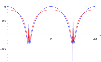
Figure 1. The two functions to integrate: the function in (2.6) [blue] and in (2.7) [red]

Integration of the two functions from $0$ to $0.999\frac{\pi}{2}\cong 1.56923$ gives for the first the value $0.999995$ and for the second the value $0.999997$. We know the last value should converge unconditionally to $\ln(\zeta(2\alpha^{\prime}))=\ln(e)=1$. This illustrate the kind of convergence involved. Notice that in both cases the “height” of integration is given by $(\frac{1}{2}-\alpha)\tan\theta\cong 117.1$, which corresponds to consider the first 37 non trivial zeros of the Zeta function.

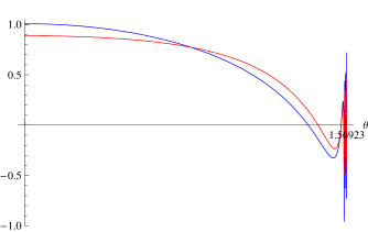
Figure 2. Plot of the two functions in the interval $[0,0.999\frac{\pi}{2}]$

Finally, we present the plot of the potentials $\varphi(\alpha)=\ln(\frac{1}{1-2\alpha})$ and $\varphi(\alpha^{\prime})=\ln(\zeta(2\alpha^{\prime}))$ which illustrate the divergence at the right border of the critical strip ($\alpha=\alpha^{\prime}=\frac{1}{2}$). We may also consider the “electrical field” inside and outside the critical strip which we define here as:

(3.1) $$E(\alpha)=\frac{d}{d\alpha}\varphi(\alpha)=\left\{\begin{array}[]{lll}\frac{2}{1-2\alpha}=2e^{\varphi(\alpha)}&,&0<\alpha<\frac{1}{2}\\ 2\frac{\zeta^{\prime}(2\alpha)}{\zeta(2\alpha)}&,&\alpha>\frac{1}{2}\end{array}\right.$$

Figure 3 summarizes the example we presented.

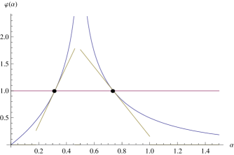
Figure 3. The potentials equal to 1 for $\alpha\cong 0.31606$ and $\alpha\cong 0.737232$ where the slopes of the two tangent straight lines are given by the magnitude of the corresponding “electrical field” defined by (3.1)

Notice that a slightly different definition of the electrical field i.e. if defined as the gradient of the potential $\varphi$ with respect to the position $\rho$ (keeping $\rho_{0}$ constant) gives the following:

(3.2) $$E(\alpha)=\frac{d}{d\rho}\varphi(\alpha)=\left\{\begin{array}[]{lll}\gamma+\frac{1}{1-\rho+\rho_{0}}&,&0<\alpha<\frac{1}{2}\\ \frac{\zeta^{\prime}(\rho+\rho_{0})}{\zeta(\rho+\rho_{0})}&,&\alpha>\frac{1}{2}\end{array}\right.$$

Moreover with our choice we obtain:

$$E(\alpha)=\left\{\begin{array}[]{lll}\gamma+\frac{1}{1-2\alpha}&,&0<\alpha<\frac{1}{2}\\ \frac{\zeta^{\prime}(2\alpha)}{\zeta(2\alpha)}&,&\alpha>\frac{1}{2}\end{array}\right.$$

4. Conclusions

In this work we have first extended some integral formulas for the logarithm of the Zeta function  by means of more general Lorentz measures and obtained two new relations equivalent to the RH. Then we have introduced a kind of “hidden symmetry” which relates the integrals between two values of the abscissa, one inside the other outside the critical strip. A simple numerical experiment has been presented as illustration of the kind of convergence involved.

We note, the truth of such a symmetry is still equivalent to the truth of the RH, but in the new formulation we have found, there is the appearance of the primes into the critical strip by means of the Zeta function calculated outside the critical strip.

The above symmetry is weaker then the stronger Riemann symmetry [6] which for the Xi  function is given pointwise by $\xi(s)=\xi(1-s)$ for any complex argument s of the Zeta function. Our weaker symmetry connects the interval [$\frac{1}{2},1$[ in the critical strip with the infinite interval ]$1,\infty$[ outside the critical strip. The work will be continued with the study of new integral relations  with a more general class of “measure” in the integration of the logarithm of the Zeta function [7].

References

• [1] F.T. Wang, A note on the Riemann Zeta-Function, Bull. Amer. Math. Soc., 52, 1946, 319-321
• [2] V.V. Volchov, On a equality equivalent to the Riemann Hypothesis, Ukranian Mathematical Journal, 47, 1995, 422
• [3] M. Balazard, E. Saias, M. Yor, Notes sur la fonction de Riemann, Advances in Mathematics, 143, 1995, 422
• [4] D. Merlini, The Riemann Magneton of the Primes, Chaos and complexity Letters, Nova Science Publishers, New York, Vol. 2, Number 1, 2006, 93
• [5] I.S. Gradshteyn, I.M. Ryzhik, Table of Integrals Series and Products, Academic Press, New York, 1965, 560
• [6] B. Riemann, Oeuvres Mathematiques, Edition Jacques Gabay, 1990, 165
• [7] S. Beltraminelli, D. Merlini, S. Sekatskii, in preparation, 2008