Discrete Affine Minimal Surfaces with Indefinite Metric

Abstract

Inspired by the Weierstrass representation of smooth affine minimal surfaces with indefinite metric, we propose a constructive process producing a large class of discrete surfaces that we call discrete affine minimal surfaces. We show that they are critical points of an affine area functional defined on the space of quadrangular discrete surfaces. The construction makes use of asymptotic coordinates and allows defining the discrete analogs of some differential geometric objects, such as the normal and co normal vector fields, the cubic form and the compatibility equations.
Keywords: Affine Minimal Surfaces, Discrete Affine Surfaces, Asymptotic coordinates

1 Introduction

In affine differential geometry, the notion of minimal surfaces, i.e. the critical points of the affine area functional, arises naturally and has received a broad attention in the last decades. In particular, it has been proved in [7],[8] that convex affine minimal surfaces actually maximize the affine area, thus justifying the sometimes used terminology maximal surfaces. On the other hand, [13] showed that this is not true for non-convex surfaces. In the convex or non-convex case, Weierstrass-type representations have been derived, allowing the explicit construction of local parameterizations of affine minimal surfaces from the co-normal vector field. This representation makes use of isothermal coordinates in the definite case and asymptotic coordinates in the indefinite case.

More recently, the expansion of computer graphics and applications in mathematical physics have given a great impulse to the issue of giving discrete equivalents of differential geometric objects ([3],[1]). In the particular case of affine geometry some work has been done toward a theory of discrete affine surfaces. In [4] a consistent definition of discrete affine spheres is proposed, both for definite and indefinite metrics and in [10] a similar construction is done in the context of improper affine spheres.

In this work we introduce a discrete analog of the smooth Weierstrass representation in the indefinite case, giving rise to explicit parameterizations of quadrangular surfaces in discrete asymptotic coordinates that we call discrete affine minimal surfaces. Over these discrete affine minimal surfaces, we can define the discrete affine metric, the discrete affine normal vector field and a discrete analog of the smooth cubic form, that we shall call discrete affine cubic form. We show that, as occurs in the smooth case, the discrete affine metric and the discrete affine cubic form must satisfy compatibility equations. Moreover, these compatibility equations are a necessary and sufficient condition for the existence of an affine minimal surface, given its metric and cubic form.

We also introduce a natural affine area functional in the set of quadrangular indefinite discrete surfaces and show that the minimal surfaces that we have constructed are critical points of this functional, thus justifying the choice of our terminology.

In view of the above results, it is natural to ask wether it is possible drop the minimality condition in this construction. This issue is related to the problem of finding a convenient definition of discrete affine mean curvature vector. In another direction, it is tempting to look for an analogous construction in the definite case. We plan to address these questions in a forthcoming work.

The paper is organized as follows: in Section 2 we state some classical notations and facts about asymptotic parameterizations of indefinite affine smooth surfaces in $\mathbb{R}^{3}.$ In Section 3, inspired by the continuous case, we implement the construction process of discrete affine minimal surfaces. Section 4 is devoted to the description of the variational property of these surfaces (Theorem 5). In last section, we introduce the discrete affine cubic form, derive the compatibility equations and prove the corresponding theorem of existence and uniqueness (Theorem 10).

2 Preliminaries

Notation. Along the paper, letters in subscripts denote partial derivatives with respect to the corresponding variable, and $V_{1}\cdot V_{2}$, $[V_{1},V_{2},V_{3}]$ and $V_{1}\times V_{2}$ denote respectively the inner product, the determinant and the cross-product of vectors $V_{1},V_{2},V_{3}\in{\mathbb{R}}^{3}$.

Consider a parameterized smooth surface $q:U\subset{\mathbb{R}}^{2}\to{\mathbb{R}}^{3}$, where $U$ is an open subset of the plane and denote by

$$L(u,v) = [q_{u},q_{v},q_{uu}]$$

$$M(u,v) = [q_{u},q_{v},q_{uv}]$$

$$N(u,v) = [q_{u},q_{v},q_{vv}]$$

The surface is non-degenerate if $LN-M^{2}\neq 0$, and, in this case, the Berwald-Blaschke metric is defined by

$$ds^{2}=\frac{1}{|LN-M^{2}|^{1/4}}\left({Ldu^{2}+2Mdudv+Ndv^{2}}\right)$$

If $LN-M^{2}>0$, the metric is definite while if $LN-M^{2}<0$, the metric is indefinite. In this paper, we shall restrict ourselves to surfaces with indefinite metric.

We say that the coordinates $(u,v)$ are asymptotic if $L=N=0$. In this case, the metric takes the form $ds^{2}=2Fdudv$, where $F^{2}=M$. Also, we can write

$$q_{uu} = \frac{1}{F}(F_{u}q_{u}+Aq_{v})$$ (1)

$$q_{vv} = \frac{1}{F}(Bq_{u}+F_{v}q_{v}),$$ (2)

where $A=A(u,v)$ and $B=B(u,v)$ are the coefficients of the affine cubic form $Adu^{3}+Bdv^{3}$ (see [12]).

The vector field $\xi(u,v)=\displaystyle{\frac{q_{uv}}{F}}$ is called the affine normal vector field. We have

$$\xi_{u} = -Hq_{u}+\frac{A_{v}}{F^{2}}q_{v}$$ (3)

$$\xi_{v} = \frac{B_{u}}{F^{2}}q_{u}-Hq_{v},$$ (4)

where $H$ is the affine mean curvature. Equations (1), (2), (3) and (4) are the structural equations of the surface. For a given surface, the quadratic form $Fdudv$, the cubic form $Adu^{3}+Bdv^{3}$ and the affine mean curvature $H$ should satisfy the following compatibility equations:

$$H_{u} = \frac{AB_{u}}{F^{3}}-\frac{1}{F}(\frac{A_{v}}{F})_{v},$$ (5)

$$H_{v} = \frac{BA_{v}}{F^{3}}-\frac{1}{F}(\frac{B_{u}}{F})_{u}.$$ (6)

Conversely, given $F,A,B$ and $H$ satisfying equations (5) and (6), there exists a parameterization $q(u,v)$ of a surface with quadratic form $2Fdudv$, cubic form $Adu^{3}+Bdv^{3}$ and affine mean curvature $H$. For details of the above equations, see [5].

The vector field $\nu(u,v)=\frac{q_{u}\times q_{v}}{F}$ is called the co-normal vector field. It satisfies Lelieuvre’s equations

$$q_{u} = \nu\times\nu_{u}$$ (7)

$$q_{v} = -\nu\times\nu_{v}.$$ (8)

It also satisfies the equation $\Delta\nu=-2H\nu$ , where $\Delta$ denotes the Laplacian with respect to the Berwald-Blaschke metric (e.g., see [12]). It turns out that in asymptotic coordinates, $\Delta\nu=\nu_{uv}$.

A surface is said to be affine minimal if its affine mean curvature $H$ vanishes or equivalently if its co-normal vector field satisfies the equation $\nu_{uv}=0$. The interest of the co-normal definition lies in the fact that the resolution of this last equation is straightforward: $\nu_{uv}=0$ if and only if $\nu(u,v)$ takes the form $\nu(u,v)=\nu^{1}(u)+\nu^{2}(v)$, where $\nu^{1}$ and $\nu^{2}$ are two real functions of one variable. Starting from the co-normal vector field and using Lelieuvre’s equations (7) and (8), one gets an immersion $q$ which turns to be a parameterization in asymptotic coordinates of an affine minimal surfaces. This is a simple way to construct examples of smooth affine minimal surfaces (e.g., see [9]).

3 Definitions, properties and examples

In this section, inspired by the properties of affine minimal surfaces and asymptotic coordinates discussed above, we describe a construction process of a class of discrete surfaces with properties analogous to the smooth case. We start with a vector field of the form $\nu(u,v)=\nu^{1}(u)+\nu^{2}(v),$ where $\nu^{1}$ and $\nu^{2}$ are two real functions of one discrete variable. In particular $\nu$ is the restriction to a subset of ${\mathbb{Z}}^{2}$ of a smooth co-normal vector field of some smooth minimal surface. To obtain the affine immersion, we make a discrete integration of the discrete analogs of Lelieuvre’s equations (7) and (8).

Notation. For a discrete real or vector function $f:D\subset{\mathbb{Z}}^{2}$, we denote the discrete partial derivatives with respect to $u$ or $v$ by

$$f_{1}(u+\tfrac{1}{2},v) = f(u+1,v)-f(u,v)$$

$$f_{2}(u,v+\tfrac{1}{2}) = f(u,v+1)-f(u,v).$$

The second order partial derivatives are defined by

$$f_{11}(u,v) = f(u+1,v)-2f(u,v)+f(u-1,v)$$

$$f_{22}(u,v) = f(u,v+1)-2f(u,v)+f(u,v-1)$$

$$f_{12}(u,v) = f(u+1,v+1)+f(u,v)-f(u+1,v)-f(u,v+1).$$

3.1 Starting with co-normals

Consider a map $\nu:D\subset{\mathbb{Z}}^{2}\to{\mathbb{R}}^{3}$, called the discrete co-normal map, satisfying

$$\nu_{12}(u+\tfrac{1}{2},v+\tfrac{1}{2})=0,\ (u,v)\in D.$$ (9)

We shall also assume that

$$F(u+\tfrac{1}{2},v+\tfrac{1}{2})=\nu(u,v)\cdot(\nu(u,v+1)\times\nu(u+1,v))>0,\ (u,v)\in D.$$

Discrete co-normal maps can be obtained from smooth maps $\nu:U\subset{\mathbb{R}}^{2}\to{\mathbb{R}}^{3}$ satisfying $\nu_{uv}=0$ by restricting the domain to a subset $D\subset{\mathbb{Z}}^{2}$.

3.2 The affine immersion

We define the affine immersion by the discrete analog of Lelieuvre¥s formulas:

$$q_{1}(u+\tfrac{1}{2},v) = \nu(u,v)\times\nu(u+1,v)$$ (10)

$$q_{2}(u,v+\tfrac{1}{2}) = -\nu(u,v)\times\nu(u,v+1).$$ (11)

Theorem 1

There exists an immersion $q(u,v)$ such that $q_{1}(u+\tfrac{1}{2},v)$ and $q_{2}(u,v+\tfrac{1}{2})$ are as above. Moreover, it satisfies the following properties:

1. The co-normal at $(u,v)$ can be obtained by any of the following formulas:

   $$\nu(u,v) = \frac{1}{F(u+\tfrac{1}{2},v+\tfrac{1}{2})}(q_{1}(u+\tfrac{1}{2},v)\times q_{2}(u,v+\tfrac{1}{2}))$$

   $$\nu(u,v) = \frac{1}{F(u-\tfrac{1}{2},v+\tfrac{1}{2})}(q_{1}(u-\tfrac{1}{2},v)\times q_{2}(u,v+\tfrac{1}{2}))$$

   $$\nu(u,v) = \frac{1}{F(u-\tfrac{1}{2},v-\tfrac{1}{2})}(q_{1}(u-\tfrac{1}{2},v)\times q_{2}(u,v-\tfrac{1}{2}))$$

   $$\nu(u,v) = \frac{1}{F(u+\tfrac{1}{2},v-\tfrac{1}{2})}(q_{1}(u+\tfrac{1}{2},v)\times q_{2}(u,v-\tfrac{1}{2})).$$

2. The parameterization is asymptotic:

   $$\left[q_{1}(u\pm\tfrac{1}{2},v),q_{2}(u,v\pm\tfrac{1}{2}),q_{11}(u,v)\right] = 0$$

   $$\left[q_{1}(u\pm\tfrac{1}{2},v),q_{2}(u,v\pm\tfrac{1}{2}),q_{22}(u,v)\right] = 0$$

   and

   $$\left[q_{1}(u+\tfrac{1}{2},v),q_{2}(u,v+\tfrac{1}{2}),q_{12}(u+\tfrac{1}{2},v+\tfrac{1}{2})\right] = F^{2}(u+\tfrac{1}{2},v+\tfrac{1}{2})$$

   $$\left[q_{1}(u+\tfrac{1}{2},v),q_{2}(u+1,v+\tfrac{1}{2}),q_{12}(u+\tfrac{1}{2},v+\tfrac{1}{2})\right] = F^{2}(u+\tfrac{1}{2},v+\tfrac{1}{2})$$

   $$\left[q_{1}(u+\tfrac{1}{2},v+1),q_{2}(u,v+\tfrac{1}{2}),q_{12}(u+\tfrac{1}{2},v+\tfrac{1}{2})\right] = F^{2}(u+\tfrac{1}{2},v+\tfrac{1}{2})$$

   $$\left[q_{1}(u+\tfrac{1}{2},v+1),q_{2}(u+1,v+\tfrac{1}{2}),q_{12}(u+\tfrac{1}{2},v+\tfrac{1}{2})\right] = F^{2}(u+\tfrac{1}{2},v+\tfrac{1}{2}).$$

• For the existence of $q$, we must show that the finite difference equations (10) and (11) are integrable, i.e., $q_{12}-q_{21}=0$. By definition,

  $$q_{12}(u+\tfrac{1}{2},v+\tfrac{1}{2}) = \nu(u,v+1)\times\nu(u+1,v+1)-\nu(u,v)\times\nu(u+1,v)$$

  $$q_{21}(u+\tfrac{1}{2},v+\tfrac{1}{2}) = -\nu(u+1,v)\times\nu(u+1,v+1)+\nu(u,v)\times\nu(u,v+1).$$

  Hence

  $$q_{12}-q_{21}=(\nu(u+1,v)+\nu(u,v+1))\times(\nu(u+1,v+1)+\nu(u,v)),$$

  which vanishes from property (9).

  We now prove only one of the equations of item 1, since the proofs of the others are similar:

  $$q_{1}(u+\tfrac{1}{2},v)\times q_{2}(u,v+\tfrac{1}{2}) = -(\nu(u,v)\times\nu(u+1,v))\times(\nu(u,v)\times\nu(u,v+1))$$

  $$= -\left[\nu(u,v),\nu(u+1,v)),\nu(u,v+1)\right]\nu(u,v)$$

  $$= F(u+\tfrac{1}{2},v+\tfrac{1}{2})\nu(u,v).$$

For the proof of item 2, we prove one formula of the first group and one formula of the second group, the others being similar:

$$L(u+\tfrac{1}{2},v+\tfrac{1}{2}) = F(u+\tfrac{1}{2},v+\tfrac{1}{2})\nu(u,v)\cdot(-q_{1}(u-\tfrac{1}{2},v))$$

$$= F(u+\tfrac{1}{2},v+\tfrac{1}{2})\nu(u,v)\cdot(\nu(u,v)\times\nu(u-1,v))=0.$$

And

$$M(u+\tfrac{1}{2},v+\tfrac{1}{2}) = F(u+\tfrac{1}{2},v+\tfrac{1}{2})\nu(u,v)\cdot(q_{2}(u+1,v+\tfrac{1}{2}))$$

$$= F(u+\tfrac{1}{2},v+\tfrac{1}{2})\nu(u,v)\cdot(\nu(u+1,v+1)\times\nu(u+1,v))$$

$$= F^{2}(u+\tfrac{1}{2},v+\tfrac{1}{2}),$$

thus completing the proof of the proposition. $\blacksquare$

The affine immersion $q:D\subset{\mathbb{Z}}^{2}\to{\mathbb{R}}^{3}$ defined by formulas (10) and (11) is called a discrete affine minimal map and its image a discrete affine minimal surface . Along this paper, when there is no risk of confusion, we shall refer to a discrete affine minimal map simply as a minimal surface.

A direct consequence of the above proposition is that $q_{1}(u+\tfrac{1}{2},v)$, $q_{1}(u+\tfrac{1}{2},v)$, $q_{1}(u+\tfrac{1}{2},v)$ and $q_{1}(u+\tfrac{1}{2},v)$ are orthogonal to $\nu(u,v)$. We shall refer to this property by saying that crosses are planar (see Figure 1). Nets with planar crosses are called asymptotic nets ([2]). It is also worthwhile to observe that the signs of $(q(u+1,v+1)-q(u,v))\cdot\nu(u,v)$, $(q(u-1,v+1)-q(u,v))\cdot\nu(u,v)$, $(q(u-1,v-1)-q(u,v))\cdot\nu(u,v)$ and $(q(u+1,v-1)-q(u,v))\cdot\nu(u,v)$ are alternating, and thus every point of the surface is a saddle point.

3.3 The affine normal map

The affine normal map $\xi(u+\tfrac{1}{2},v+\tfrac{1}{2})$ is defined to be

$$\xi(u+\tfrac{1}{2},v+\tfrac{1}{2})=\frac{q_{12}(u+\tfrac{1}{2},v+\tfrac{1}{2})}{F(u+\tfrac{1}{2},v+\tfrac{1}{2})}$$

Proposition 2

The affine normal enjoys the following properties :

1. $$\nu(u,v)\cdot\xi(u+\tfrac{1}{2},v+\tfrac{1}{2}) = 1$$

   $$\nu(u+1,v)\cdot\xi(u+\tfrac{1}{2},v+\tfrac{1}{2}) = 1$$

   $$\nu(u,v+1)\cdot\xi(u+\tfrac{1}{2},v+\tfrac{1}{2}) = 1$$

   $$\nu(u+1,v+1)\cdot\xi(u+\tfrac{1}{2},v+\tfrac{1}{2}) = 1.$$

2. $$\nu_{1}(u+\tfrac{1}{2},v)\times\nu_{2}(u,v+\tfrac{1}{2}) = -F(u+\tfrac{1}{2},v+\tfrac{1}{2})\xi(u+\tfrac{1}{2},v+\tfrac{1}{2})$$

   $$\nu_{1}(u+\tfrac{1}{2},v)\times\nu_{2}(u+1,v+\tfrac{1}{2}) = -F(u+\tfrac{1}{2},v+\tfrac{1}{2})\xi(u+\tfrac{1}{2},v+\tfrac{1}{2})$$

   $$\nu_{1}(u+\tfrac{1}{2},v+1)\times\nu_{2}(u,v+\tfrac{1}{2}) = -F(u+\tfrac{1}{2},v+\tfrac{1}{2})\xi(u+\tfrac{1}{2},v+\tfrac{1}{2})$$

   $$\nu_{1}(u+\tfrac{1}{2},v+1)\times\nu_{2}(u+1,v+\tfrac{1}{2}) = -F(u+\tfrac{1}{2},v+\tfrac{1}{2})\xi(u+\tfrac{1}{2},v+\tfrac{1}{2}).$$

• All formulas of Item 1 follow directly from the equation

  $$q_{12}(u+\tfrac{1}{2},v+\tfrac{1}{2})=\nu(u,v+1)\times\nu(u+1,v+1)-\nu(u,v)\times\nu(u+1,v).$$

  For the second Item, we shall prove one of the equations, the others being similar:

  $$\nu_{1}(u+\tfrac{1}{2},v)\times\nu_{2}(u+1,v+\tfrac{1}{2}) = \nu(u+1,v)\times\nu(u,v+1)-\nu(u+1,v)\times\nu(u,v)-\nu(u,v)\times\nu(u,v+1)$$

  $$= -q_{12}(u+\tfrac{1}{2},v+\tfrac{1}{2})$$

  $$= -F(u+\tfrac{1}{2},v+\tfrac{1}{2})\xi(u+\tfrac{1}{2},v+\tfrac{1}{2}),$$

  thus proving the proposition. $\blacksquare$

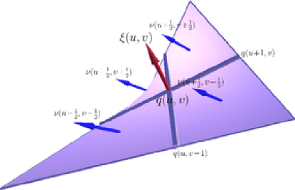
Figure 1: The planar cross, the co-normal vector at the vertex and the normal vectors at the faces.

3.4 Bi-linear interpolation

The bi-linear interpolation between four points $q(u,v)$, $q(u+1,v)$, $q(u,v+1)$ and $q(u+1,v+1)$ suits very well to the discrete affine minimal surface with indefinite metric. This interpolation generates a continuous surface and respects the normal and co-normal vectors. All figures of this paper were computed using this interpolation.

A parameterization of the hyperbolic paraboloid that passes through $q(u,v)$, $q(u+1,v)$, $q(u,v+1)$ and $q(u+1,v+1)$ is given by

$$r(s,t)=q(u,v)+s(q(u\!+\!1,v)-q(u,v))+t(q(u,v\!+\!1)-q(u,v))+st(q(u\!+\!1,v\!+\!1)+q(u,v)-q(u\!+\!1,v)-q(u,v\!+\!1)),$$ (12)

for $0\leq s\leq 1$, $0\leq t\leq 1$.

Lemma 3

The parameterization (12) is asymptotic and the affine area of the quadratic patch is exactly $F(u+\tfrac{1}{2},v+\tfrac{1}{2})$. Also, $\xi(u+\tfrac{1}{2},v+\tfrac{1}{2})$ is the constant affine normal of the surface, and the co-normals at the corners coincide with $\nu(u,v)$, $\nu(u+1,v)$, $\nu(u,v+1)$ and $\nu(u+1,v+1)$.

• Direct calculations shows that the area element of the surface defined by (12) is $F(u+\tfrac{1}{2},v+\tfrac{1}{2})dsdt$ and thus its affine area is $F(u+\tfrac{1}{2},v+\tfrac{1}{2})$. The calculation of the affine normal and the co-normals at the corners are straightforward. $\blacksquare$

3.5 Examples

Example 1

The smooth helicoid can be parameterized in asymptotic coordinates by

$$q(u,v)=(u\cos(v),u\sin(v),v),\ (u,v)\in{\mathbb{R}}^{2},$$

and its co-normal vector field is $\nu(u,v)=(\sin(v),-\cos(v),u)$. In order to obtain a discrete counterpart of the helicoid, we integrate the map $\nu(u,v)=(\sin(\frac{2\pi}{N}v),-\cos(\frac{2\pi}{N}v),u)$ for $(u,v)\in{\mathbb{Z}}\times[0,N]\subset{\mathbb{Z}}^{2}$. The resulting discrete helicoid is shown in Figure 2, together with the smooth one. We observe that the discrete parameterizations are not restrictions to ${\mathbb{Z}}^{2}$ of the smooth parameterization, i.e., the vertices of the discrete surfaces are not points of the smooth surface.

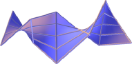
(a) Discrete helicoid.

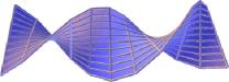
(b) Discrete helicoid at a higher resolution.

(c) Smooth helicoid.

Figure 2: Discrete helicoid in two resolutions and the smooth one.

Example 2

Consider a smooth vector field $\nu(u,v)=(u,v,u^{2}+v^{2})$, $(u,v)\in{\mathbb{R}}^{2}$. The associated smooth immersion is given by

$$q(u,v)=(u^{2}v-\frac{v^{3}}{3},v^{2}u-\frac{u^{3}}{3},-uv).$$

To obtain the discrete counterpart of this minimal surface, we make a discrete integration of $\nu(u,v)=(u,v,u^{2}+v^{2})$, $(u,v)\in{\mathbb{Z}}^{2}$. The resulting discrete surface, together with the smooth one, is shown in Figure 3. Again, the vertices of the discrete surface are not points of the smooth surface.

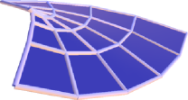
(a) Discrete minimal cubic.

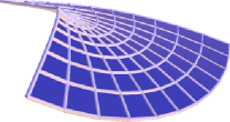
(b) Discrete minimal cubic in higher resolution.

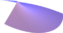
(c) Smooth minimal cubic.

Figure 3: Discrete minimal cubic in two resolutions and smooth minimal cubic.

Example 3

The hyperbolic paraboloid can be parameterized in asymptotic coordinates by

$$q(u,v)=(u,v,uv),\ (u,v)\in{\mathbb{R}}^{2},$$

and its co-normal vector field is $\nu(u,v)=(-v,-u,1)$. If we integrate the restriction of $\nu$ to ${\mathbb{Z}}^{2}$, we obtain a discrete minimal surface. It turns out that in this special case, the discrete immersion is the restriction to ${\mathbb{Z}}^{2}$ of the smooth immersion. Moreover, we observe that if we interpolate this discrete surface as in subsection 3.4, we obtain again the smooth hyperbolic paraboloid (see Figure 4).

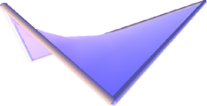
(a) Discrete hyperbolic paraboloid.

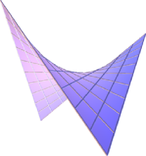
(b) Discrete hyperbolic paraboloid in higher resolution.

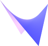
(c) Smooth hyperbolic paraboloid.

Figure 4: The discrete hyperbolic paraboloid and the smooth one coincides.

A discrete improper affine sphere is a discrete minimal surface for which the affine normal vector field is constant. It can also be characterized by the fact that the co-normal vector field is contained in a plane.

Example 4

Consider $\nu(u,v)=(\frac{v^{2}-u^{2}}{4},\frac{u-v}{2},-1)$. The corresponding smooth affine immersion is

$$q(u,v)=(\frac{u+v}{2},\frac{u^{2}+v^{2}}{4},\frac{(u-v)^{3}}{24}),$$

and it is defined only for $u>v$. It is an improper affine sphere, since the image of the co-normal vector field is contained in a plane. This surface is the graph of the area distance (see [11]), a well-known concept in computer vision, to the parabola $(t,\frac{t^{2}}{2})$, $t\in{\mathbb{R}}$ . The corresponding discrete immersion is the graph of the area distance of the polygon defined by $(t,\frac{t^{2}}{2})$, $t\in{\mathbb{Z}}$ (for details, see [6]). The smooth and discrete surfaces are shown in Figure 5.

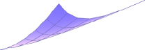
(a) Discrete affine sphere.

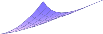
(b) Discrete affine sphere in higher resolution.

(c) Smooth affine sphere.

Figure 5: The discrete and smooth affine spheres.

4 Variational property

In this section we introduce a functional on the space of discrete indefinite quadrangular surfaces and prove that the affine minimal discrete surfaces that we have described in Section 3 are actually critical points of this functional.

4.1 The discrete affine area functional

Let $S$ a discrete quadrangular surface and $q:D\to{\mathbb{R}}^{3},$ with $D\subset{\mathbb{Z}}^{2}$ a parameterization of $S$. We further assume that for any $(u,v)\in D,$ the quantity

$$M(u,v)=\big{[}q(u+1,v)-q(u,v),q(u,v+1)-q(u,v),q(u+1,v+1)-q(u,v)\big{]}$$

is strictly positive. The quantity $F=\sqrt{M}$ is the affine area of the hyperbolic paraboloid that passes through the vertices $q(u,v),q(u+1,v),q(u,v+1)$ and $q(u+1,v+1).$ The affine area of $S$ is defined as

$${\cal F}(S)=\sum_{(u,v)\in D}F(u,v).$$

Let $V(u,v):D\to{\mathbb{R}}^{3}$ a map such that $V(u,v)$ vanishes except on a finite number of points $(u,v)$ of $D$. Intuitively, $V$ must be regarded as a compactly supported vector field on $S$. The surface $S(t)$ parameterized by $q_{t}(u,v)=q(u,v)+tV(u,v)$ is a deformation of $S.$ For $t$ small enough, we still have $M_{t}(u,v)>0,$ so the next definition makes sense:

Definition 4

A quadrangular surface is said to be variationally discrete affine minimal if

$$\left.\frac{d{\cal F}(S_{t})}{dt}\right|_{t=0}=0,$$

for any such deformation.

Theorem 5

Let $q:D\subset{\mathbb{Z}}^{2}\to{\mathbb{R}}^{3}$ be a discrete affine minimal immersion as defined in Section 3. Then it is variationally minimal.

• We first observe that the first variation $\left.\frac{d{\cal F}(S_{t})}{dt}\right|_{t=0}$ is linear with respect to $V,$ so that it is sufficient to look at a point-wise deformation. Let $(q_{0},q_{1},q_{2},q_{3})$ be a quadrangle, whose last vertex $q_{3}(t)$ is deformed by

  $$q_{3}(t)=q_{3}(0)+tV+o(t),$$

  i.e. $q_{3}^{\prime}(0)=V$. Since $F^{2}(t)=[q_{1}-q_{0},q_{2}-q_{0},q_{3}(t)-q_{0}]$, we obtain

  $$F^{\prime}(0)=(\frac{(q_{1}-q_{0})\times(q_{2}-q_{0})}{2F(0)})\cdot V.$$

If a vertex $q(u,v)$ is deformed by

$$q(u,v,t)=q(u,v)+tV+o(t),$$

it affects the affine area of its four neighbors quadrangles. The area variation of the quadrangle $(u-\tfrac{1}{2},v-\tfrac{1}{2})$ is given by $h_{1}\cdot V$, where

$$h_{1}=\frac{q_{1}(u-\tfrac{1}{2},v-1)\times q_{2}(u-1,v-\tfrac{1}{2})}{2F(u-\tfrac{1}{2},v-\tfrac{1}{2})}$$

Similarly, the area variations of the quadrangles $(u+\tfrac{1}{2},v-\tfrac{1}{2})$, $(u+\tfrac{1}{2},v+\tfrac{1}{2})$ and $(u-\tfrac{1}{2},v+\tfrac{1}{2})$ are given by $h_{2}\cdot V$, $h_{3}\cdot V$ and $h_{4}\cdot V$, where

$$h_{2} = -\frac{q_{1}(u+\tfrac{1}{2},v-1)\times q_{2}(u+1,v-\tfrac{1}{2})}{2F(u+\tfrac{1}{2},v-\tfrac{1}{2})}$$

$$h_{3} = \frac{q_{1}(u+\tfrac{1}{2},v+1)\times q_{2}(u+1,v+\tfrac{1}{2})}{2F(u+\tfrac{1}{2},v+\tfrac{1}{2})}$$

$$h_{4} = -\frac{q_{1}(u-\tfrac{1}{2},v+1)\times q_{2}(u-1,v+\tfrac{1}{2})}{2F(u-\tfrac{1}{2},v+\tfrac{1}{2})}.$$

Since $\left.\frac{d{\cal F}(S_{t})}{dt}\right|_{t=0}=(h_{1}+h_{2}+h_{3}+h_{4})\cdot V$, the surface is variationally minimal if and only if $h_{1}+h_{2}+h_{3}+h_{4}=0$, for any $(u,v)\in D$.

Assuming that $S$ is affine minimal, we have that

$$\nu(u+1,v+1)+\nu(u,v)-\nu(u,v+1)-\nu(u+1,v)=0,$$

for any $(u,v)\in D$, implying that

$$\nu(u-1,v-1)+\nu(u+1,v+1)-\nu(u-1,v+1)-\nu(u+1,v-1)=0,$$

for any $(u,v)\in D$, which, by Proposition 1, is equivalent to $h_{1}+h_{2}+h_{3}+h_{4}=0$. $\blacksquare$

5 Structural equations and compatibility

In this section we define the discrete affine cubic form and show that any discrete affine minimal surface must satisfy compatibility equations that involve also the discrete quadratic form, i.e., the Berwald-Blaschke metric. On the other hand, given discrete quadratic and cubic forms satisfying the compatibility equations, there exists a discrete affine minimal surface, unique up to affine transformations of ${\mathbb{R}}^{3}$, with the given quadratic and cubic forms. This result is the discrete counterpart of the structural theorem for smooth affine minimal surfaces.

5.1 The discrete cubic form

We define the discrete cubic form as $A(u,v)\delta u^{3}+B(u,v)\delta v^{3}$, where

$$A(u,v) = [q_{1}(u-\tfrac{1}{2},v),q_{1}(u+\tfrac{1}{2},v),\xi(u\pm\tfrac{1}{2},v\pm\tfrac{1}{2})]$$

$$B(u,v) = [q_{2}(u,v+\tfrac{1}{2}),q_{2}(u,v-\tfrac{1}{2}),\xi(u\pm\tfrac{1}{2},v\pm\tfrac{1}{2})].$$

Since we are interested only in the coefficients $A(u,v)$ and $B(u,v)$ of the discrete cubic form, we shall not discuss in this paper the meaning of the symbols $\delta u^{3}$ and $\delta v^{3}$.

From the definition of $A$ and $B$, we can write

$$q_{11}(u,v) = \frac{1}{F(u+\tfrac{1}{2},v+\tfrac{1}{2})}(F_{1}(u,v+\tfrac{1}{2})q_{1}(u+\tfrac{1}{2},v)+A(u,v)q_{2}(u,v+\tfrac{1}{2}))$$

$$= \frac{1}{F(u-\tfrac{1}{2},v+\tfrac{1}{2})}(F_{1}(u,v+\tfrac{1}{2})q_{1}(u-\tfrac{1}{2},v)+A(u,v)q_{2}(u,v+\tfrac{1}{2}))$$

$$= \frac{1}{F(u+\tfrac{1}{2},v-\tfrac{1}{2})}(F_{1}(u,v-\tfrac{1}{2})q_{1}(u+\tfrac{1}{2},v)+A(u,v)q_{2}(u,v-\tfrac{1}{2}))$$

$$= \frac{1}{F(u-\tfrac{1}{2},v-\tfrac{1}{2})}(F_{1}(u,v-\tfrac{1}{2})q_{1}(u-\tfrac{1}{2},v)+A(u,v)q_{2}(u,v-\tfrac{1}{2}))$$

$$q_{22}(u,v) = \frac{1}{F(u+\tfrac{1}{2},v+\tfrac{1}{2})}(B(u,v)q_{1}(u+\tfrac{1}{2},v)+F_{2}(u+\tfrac{1}{2},v)q_{2}(u,v+\tfrac{1}{2}))$$

$$= \frac{1}{F(u-\tfrac{1}{2},v+\tfrac{1}{2})}(B(u,v)q_{1}(u-\tfrac{1}{2},v)+F_{2}(u-\tfrac{1}{2},v)q_{2}(u,v+\tfrac{1}{2}))$$

$$= \frac{1}{F(u+\tfrac{1}{2},v-\tfrac{1}{2})}(B(u,v)q_{1}(u+\tfrac{1}{2},v)+F_{2}(u+\tfrac{1}{2},v)q_{2}(u,v-\tfrac{1}{2}))$$

$$= \frac{1}{F(u-\tfrac{1}{2},v-\tfrac{1}{2})}(B(u,v)q_{1}(u-\tfrac{1}{2},v)+F_{2}(u-\tfrac{1}{2},v)q_{2}(u,v-\tfrac{1}{2})),$$

where $F_{1}(u,v+\tfrac{1}{2})=F(u+\tfrac{1}{2},v+\tfrac{1}{2})-F(u-\tfrac{1}{2},v+\tfrac{1}{2})$ and $F_{2}(u+\tfrac{1}{2},v)=F(u+\tfrac{1}{2},v+\tfrac{1}{2})-F(u+\tfrac{1}{2},v-\tfrac{1}{2})$.

5.2 Derivatives of the affine normal

We shall now calculate the derivatives of the affine normal. We first prove a technical lemma:

Lemma 6

The discrete derivatives $A_{2}$ and $B_{1}$ can be expressed as:

$$A_{2}(u,v+\tfrac{1}{2}) = F(u-\tfrac{1}{2},v+\tfrac{1}{2})[q_{1}(u+\tfrac{1}{2},v),\xi(u-\tfrac{1}{2},v+\tfrac{1}{2}),\xi(u+\tfrac{1}{2},v+\tfrac{1}{2})]$$

$$B_{1}(u+\tfrac{1}{2},v) = -F(u+\tfrac{1}{2},v-\tfrac{1}{2})[q_{2}(u,v+\tfrac{1}{2}),\xi(u+\tfrac{1}{2},v-\tfrac{1}{2}),\xi(u+\tfrac{1}{2},v+\tfrac{1}{2})].$$

• We can write

  $$q_{1}(u-\tfrac{1}{2},v)\times q_{1}(u+\tfrac{1}{2},v)=A(u,v)\nu(u,v)$$

  Differentiating with respect to $v$ we obtain

  $$A(u,v+1)\nu(u,v+1)-A(u,v)\nu(u,v)=q_{1}(u-\tfrac{1}{2},v+1)\times q_{1}(u+\tfrac{1}{2},v+1)-q_{1}(u-\tfrac{1}{2},v)\times q_{1}(u+\tfrac{1}{2},v)$$

  Multiplying by $\xi(u+\tfrac{1}{2},v+\tfrac{1}{2})$ we have

  $$A(u,v+1)-A(u,v) = [q_{1}(u-\tfrac{1}{2},v+1)\times q_{1}(u+\tfrac{1}{2},v+1)-q_{1}(u-\tfrac{1}{2},v)\times q_{1}(u+\tfrac{1}{2},v)]\cdot\xi(u+\tfrac{1}{2},v+\tfrac{1}{2})$$

  $$= [q_{1}(u-\tfrac{1}{2},v+1)-q_{1}(u-\tfrac{1}{2},v),q_{1}(u+\tfrac{1}{2},v),\xi(u+\tfrac{1}{2},v+\tfrac{1}{2})]$$

  $$= -F(u-\tfrac{1}{2},v+\tfrac{1}{2})[\xi(u-\tfrac{1}{2},v+\tfrac{1}{2}),q_{1}(u+\tfrac{1}{2},v),\xi(u+\tfrac{1}{2},v+\tfrac{1}{2})]$$

  The calculation for $B_{1}$ is similar. $\blacksquare$

Observe that $\nu(u,v)\cdot\xi_{1}(u,v+\tfrac{1}{2})=\nu(u,v)\cdot\xi_{2}(u+\tfrac{1}{2},v)=0$, and thus we can write $\xi_{1}(u,v+\tfrac{1}{2})$ and $\xi_{2}(u+\tfrac{1}{2},v)$ as linear combinations of $q_{1}(u+\tfrac{1}{2},v)$ and $q_{2}(u,v+\tfrac{1}{2}))$. More precisely, we have the following proposition:

Proposition 7

The discrete derivatives of the affine normals can be expressed as:

$$F(u-\tfrac{1}{2},v+\tfrac{1}{2})F(u+\tfrac{1}{2},v+\tfrac{1}{2})\xi_{1}(u,v+\tfrac{1}{2}) = -A_{2}(u,v+\tfrac{1}{2})q_{2}(u,v+\tfrac{1}{2})$$ (13)

$$F(u+\tfrac{1}{2},v-\tfrac{1}{2})F(u+\tfrac{1}{2},v+\tfrac{1}{2})\xi_{2}(u+\tfrac{1}{2},v) = -B_{1}(u+\tfrac{1}{2},v)q_{1}(u+\tfrac{1}{2},v).$$ (14)

• We first show that the coefficient of $q_{1}(u+\tfrac{1}{2},v)$ in the expansion of $\xi_{1}(u,v+\tfrac{1}{2})$ is zero. We have

  $$[\xi_{1}(u,v+\tfrac{1}{2}),q_{2}(u,v+\tfrac{1}{2}),\xi(u+\tfrac{1}{2},v+\tfrac{1}{2})] = -[\xi(u-\tfrac{1}{2},v+\tfrac{1}{2}),q_{2}(u,v+\tfrac{1}{2}),\xi(u+\tfrac{1}{2},v+\tfrac{1}{2})]$$

  $$= \frac{[q_{2}(u-1,v+\tfrac{1}{2}),q_{2}(u,v+\tfrac{1}{2}),q_{2}(u+1,v+\tfrac{1}{2})]}{F(u-\tfrac{1}{2},v+\tfrac{1}{2})F(u+\tfrac{1}{2},v+\tfrac{1}{2})}$$

  And

  $$q_{2}(u-1,v+\tfrac{1}{2})\times q_{2}(u,v+\tfrac{1}{2}) = (\nu(u-1,v+1)\times\nu(u-1,v))\times(\nu(u,v+1)\times\nu(u,v))$$

  $$= ((\nu(u,v+1)-\nu(u,v))\times\nu(u-1,v))\times(\nu(u,v+1)\times\nu(u,v))$$

  $$= -F(u-\tfrac{1}{2},v+\tfrac{1}{2})(\nu(u,v+1)-\nu(u,v))$$

  So

  $$[\xi_{1}(u,v+\tfrac{1}{2}),q_{2}(u,v+\tfrac{1}{2}),\xi(u+\tfrac{1}{2},v+\tfrac{1}{2})] = -\frac{(\nu(u,v+1)-\nu(u,v))\cdot(\nu(u+1,v+1)\times\nu(u+1,v))}{F(u+\tfrac{1}{2},v+\tfrac{1}{2})}$$

  $$= -\frac{1}{F(u+\tfrac{1}{2},v+\tfrac{1}{2})}(F(u+\tfrac{1}{2},v+\tfrac{1}{2})-F(u+\tfrac{1}{2},v+\tfrac{1}{2}))=0.$$

  We can now easily complete the proof of the first equation using lemma 6. The proof of the second equation is similar. $\blacksquare$

Corollary 8

A discrete affine minimal surface is an improper affine sphere if and only if $A=A(u)$ and $B=B(v)$.

5.3 Compatibility equations

In this subsection we obtain three compatibility equations. They are generalizations of the equations obtained in [10] for discrete improper affine spheres. The first equation is proved in the following lemma:

Lemma 9

$$F(u-\tfrac{1}{2},v+\tfrac{1}{2})F(u+\tfrac{1}{2},v-\tfrac{1}{2})-F(u+\tfrac{1}{2},v+\tfrac{1}{2})F(u-\tfrac{1}{2},v-\tfrac{1}{2})=A(u,v)B(u,v).$$ (15)

• We can calculate $q_{112}(u,v+\tfrac{1}{2})$ as $q_{12}(u+\tfrac{1}{2},v+\tfrac{1}{2})-q_{12}(u-\tfrac{1}{2},v+\tfrac{1}{2})$ and also as $q_{11}(u,v+1)-q_{11}(u,v)$. Calculating in the first way, we have from $q_{12}=F\xi$ that

  $$q_{112}(u,v+\tfrac{1}{2}) = F_{1}(u,v+\tfrac{1}{2})\xi(u+\tfrac{1}{2},v+\tfrac{1}{2})+F(u+\tfrac{1}{2},v+\tfrac{1}{2})\xi_{1}(u,v+\tfrac{1}{2})$$

  $$= F_{1}(u,v+\tfrac{1}{2})\xi(u+\tfrac{1}{2},v+\tfrac{1}{2})-\frac{A_{2}(u,v+\tfrac{1}{2})}{F(u-\tfrac{1}{2},v+\tfrac{1}{2})}q_{2}(u,v+\tfrac{1}{2}).$$

  Calculating in the second way, formulas of subsection 5.1 imply that

  $$q_{112}(u,v+\tfrac{1}{2}) = \left(\frac{F_{1}(u,v+\tfrac{1}{2})}{F(u+\tfrac{1}{2},v+\tfrac{1}{2})}-\frac{F_{1}(u,v-\tfrac{1}{2})}{F(u+\tfrac{1}{2},v-\tfrac{1}{2})}\right)q_{1}(u+\tfrac{1}{2},v)+F_{1}(u,v+\tfrac{1}{2})\xi(u+\tfrac{1}{2},v+\tfrac{1}{2})$$

  $$+ \left(\frac{A(u,v+1)}{F(u+\tfrac{1}{2},v+\tfrac{1}{2})}-\frac{A(u,v)}{F(u+\tfrac{1}{2},v-\tfrac{1}{2})}\right)q_{2}(u,v+\tfrac{1}{2})+\frac{A(u,v)}{F(u+\tfrac{1}{2},v-\tfrac{1}{2})}q_{22}(u,v)$$

  Now, using the formula for $q_{22}(u,v)$ and comparing the coefficients of $q_{1}(u+\tfrac{1}{2},v)$, we obtain

  $$A(u,v)B(u,v)+F_{1}(u,v+\tfrac{1}{2})F(u+\tfrac{1}{2},v-\tfrac{1}{2})-F_{1}(u,v-\tfrac{1}{2})F(u+\tfrac{1}{2},v+\tfrac{1}{2})=0,$$

  thus proving the lemma.

  $\blacksquare$

The two other compatibility equations are obtained from Equations (13) and (14). We can write

$$F(u+\tfrac{1}{2},v+\tfrac{1}{2})\xi_{12}(u,v) = -\frac{B(u,v)A_{2}(u,v-\tfrac{1}{2})}{F(u-\tfrac{1}{2},v-\tfrac{1}{2})F(u+\tfrac{1}{2},v-\tfrac{1}{2})}q_{1}(u+\tfrac{1}{2},v)$$

$$+ \left(\frac{A_{2}(u,v-\tfrac{1}{2})}{F(u-\tfrac{1}{2},v-\tfrac{1}{2})}-\frac{A_{2}(u,v+\tfrac{1}{2})}{F(u-\tfrac{1}{2},v+\tfrac{1}{2})}\right)q_{2}(u,v+\tfrac{1}{2})$$

$$F(u+\tfrac{1}{2},v+\tfrac{1}{2})\xi_{21}(u,v) = \left(\frac{B_{1}(u-\tfrac{1}{2},v)}{F(u-\tfrac{1}{2},v-\tfrac{1}{2})}-\frac{B_{1}(u+\tfrac{1}{2},v)}{F(u+\tfrac{1}{2},v-\tfrac{1}{2})}\right)q_{1}(u+\tfrac{1}{2},v)$$

$$- \frac{A(u,v)B_{1}(u-\tfrac{1}{2},v)}{F(u-\tfrac{1}{2},v-\tfrac{1}{2})F(u-\tfrac{1}{2},v+\tfrac{1}{2})}q_{2}(u,v+\tfrac{1}{2}).$$

Thus we get

$$F(u-\tfrac{1}{2},v-\tfrac{1}{2})B_{1}(u+\tfrac{1}{2},v)-F(u+\tfrac{1}{2},v-\tfrac{1}{2})B_{1}(u-\tfrac{1}{2},v) = B(u,v)A_{2}(u,v-\tfrac{1}{2})$$ (16)

$$F(u-\tfrac{1}{2},v-\tfrac{1}{2})A_{2}(u,v+\tfrac{1}{2})-F(u-\tfrac{1}{2},v+\tfrac{1}{2})A_{2}(u,v-\tfrac{1}{2}) = A(u,v)B_{1}(u-\tfrac{1}{2},v).$$ (17)

5.4 Existence and uniqueness theorem

In this subsection, we prove the existence and uniqueness of a discrete affine minimal surface with given quadratic and cubic forms satisfying the compatibility equations.

Theorem 10

Given function $F(u+\tfrac{1}{2},v+\tfrac{1}{2})$, $A(u,v)$ and $B(u,v)$ satisfying the compatibility equations (15), (16) and (17), there exists a discrete affine minimal surface $q(u,v)$ with quadratic form $Fdudv$ and cubic form $A\delta u^{3}+B\delta v^{3}$. Moreover, two discrete affine minimal surfaces with the same quadratic and cubic forms are affine equivalent.

• We begin by choosing four points $q(0,0)$, $q(1,0)$, $q(0,1)$ and $q(1,1)$ satisfying $[q(1,0)-q(0,0),q(0,1)-q(0,0),q(1,1)-q(0,0)]=F^{2}(\tfrac{1}{2},\tfrac{1}{2})$. This four points are determined up to an affine transformation of ${\mathbb{R}}^{3}$.

  From a quadrangle $(u-\tfrac{1}{2},v-\tfrac{1}{2})$, one can extend the definition of $q$ to the quadrangles $(u+\tfrac{1}{2},v-\tfrac{1}{2})$ and $(u-\tfrac{1}{2},v+\tfrac{1}{2})$ by the formulas of Section 5.1. With these extensions, we can calculate $\xi(u+\tfrac{1}{2},v-\tfrac{1}{2})$ and $\xi(u-\tfrac{1}{2},v+\tfrac{1}{2})$. It is clear that $\xi_{1}(u,v-\tfrac{1}{2})$ and $\xi_{2}(u-\tfrac{1}{2},v)$ satisfy equations (13) and (14). The coherence of these extensions are assured by formula (15).

Then one can extend the definition of $q$ to $(u+\tfrac{1}{2},v+\tfrac{1}{2})$ in two different ways: from the quadrangle $(u+\tfrac{1}{2},v-\tfrac{1}{2})$ and from the $(u-\tfrac{1}{2},v+\tfrac{1}{2})$. Our task is to show that both extensions leads to the same result. This amounts to check that both affine normals $\xi(u+\tfrac{1}{2},v+\tfrac{1}{2})$ are the same, which in fact reduces to verify that $\xi_{12}=\xi_{21}$. But this last equation holds by the compatibility hypothesis, which completes the proof of the theorem. $\blacksquare$

Acknowledgements. The first and third authors want to thank CNPq for financial support during the preparation of this paper.

References

- [1] A. Bobenko, P. Schröder, J. Sullivan, and G. Ziegler, editors. Discrete Differential Geometry, volume 38 of Oberwolfach Seminars. Birkhauser, 2008.
- [2] A. I. Bobenko and Y. B.Suris. Discrete differential geometry: Consistency as integrability. pre-print, 2005.
- [3] A. I. Bobenko, T. Hoffmann, and B. A. Springborn. Minimal surfaces from circle patterns: Geometry from combinatorics. Annals of Mathematics, 164(1):231–264, 2006.
- [4] A. I. Bobenko and W. K. Schief. Affine spheres: Discretization via duality relations. Experimental Mathematics, 8(3):261–280, 1999.
- [5] S. Buchin. Affine Differential Geometry. Science Press, Beijing, China, Gordon and Breach,Science Publishers, New York, 1983.
- [6] M. Craizer, M. A. da Silva, and R. C. Teixeira. Area distances of convex plane curves and improper affine spheres. pre-print, 2008.
- [7] E.Calabi. Hypersurfaces with maximal affinely invariant area. American Journal of Mathematics, 104:91–126, 1982.
- [8] E.Calabi. Convex affine maximal surfaces. Results in Mathematics, 13:199–223, 1988.
- [9] A.-M. Li, U. Simon, and G. Zhao. Global Affine Differential Geometry of Hypersurfaces. De Gruyter Expositions in Mathematics, 1993.
- [10] N. Matsuura and H. Urakawa. Discrete improper affine spheres. Journal of Geometry and Physics, 45:164–183, 2003.
- [11] M. Niethammer, S. Betelu, G. Sapiro, A. Tannenbaum, and P. J. Giblin. Area-based medial axis of planar curves. International Journal of Computer Vision, 60(3):203–224, 2004.
- [12] K. Nomizu and T. Sasaki. Affine Differential Geometry. Cambridge University Press, 1994.
- [13] L. Verstraelen and L. Vrancken. Affine variation formulas and affine minimal surfaces. Michigan Mathematical Journal, 36:77–93, 1989.