Evolution from BCS to BKT superfluidity in one-dimensional optical lattices

Abstract

We analyze the finite temperature phase diagram of fermion mixtures in one-dimensional optical lattices as a function of interaction strength. At low temperatures, the system evolves from an anisotropic three-dimensional Bardeen-Cooper-Schrieffer (BCS) superfluid to an effectively two-dimensional Berezinskii-Kosterlitz-Thouless (BKT) superfluid as the interaction strength increases. We calculate the critical temperature as a function of interaction strength, and identify the region where the dimensional crossover occurs for a specified optical lattice potential. Finally, we show that the dominant vortex excitations near the critical temperature evolve from multiplane elliptical vortex loops in the three-dimensional regime to planar vortex-antivortex pairs in the two-dimensional regime, and we propose a detection scheme for these excitations.

Ultracold atoms in optical lattices are ideal systems to simulate and study novel and exotic condensed matter phases. Remarkable success has been achieved experimentally with Bose atoms loaded into three-dimensional (3D) optical lattices, where superfluid and Mott-insulator phases have been observed bloch-2005 . In addition, experimental evidence for superfluid and possibly insulating phases were found for fermionic atoms (⁶Li) in 3D optical lattices ketterle-2006 . Compared with the purely homogeneous or harmonically trapped systems, optical lattices offer additional flexibilities and an unprecedented degree of control such that their physical properties can be studied as a function of onsite atom-atom interactions, tunneling amplitudes between adjacent sites, atom filling fractions and lattice dimensionality.

For instance, in strictly two-dimensional (2D) systems the superfluid transition for bosons and fermions is of the Berezinskii-Kosterlitz-Thouless (BKT) type berezinskii-1971 ; kosterlitz-1972 . This phase is characterized by the existence of bound vortex-antivortex pairs below the critical temperature $T_{BKT}$, and evidence for it was recently reported in nearly 2D Bose gases confined to one-dimensional (1D) optical lattices zoran-2006 . Thus, it is very likely that one of the next research frontiers for experiments with fermions in optical lattices is also the investigation of such a transition.

For bosons or fermions, it is possible to study not only 3D and 2D superfluids as two separate limits, but also the entire evolution from 3D to 2D by tuning nearly continuously the tunneling amplitudes stoferle-2006 ; bongs-2006 . However, fermions offer the additional advantage that their interactions can also be tuned using Feshbach resonances without having to worry about the collapse of the condensate, as it is the case for bosons. Furthermore, the phase diagram of fermions in optical lattices also shows superfluid-to-insulator transitions iskin-2007 ; ho-2007 ; sachdev-2007 like bosons do.

Anticipating experiments, we study in this manuscript the finite temperature phase diagram of attractive fermion mixtures in 1D optical lattices, and discuss the dimensional crossover from an anisotropic-3D BCS superfluid to an effectively 2D BKT superfluid as a function of interaction strength and tunneling parameters. We show that vortex excitations near the critical temperature change from elliptical multiplane vortex loops in the anisotropic-3D BCS regime to planar vortex-antivortex pairs in the 2D BKT regime. Finally, we propose an experiment for the detection of vortex excitations.

To describe fermion mixtures in 1D optical lattices, we start with the Hamiltonian ($\hbar=k_{B}=1$)

$$H=\sum_{\mathbf{k},\sigma}\xi_{\mathbf{k},\sigma}a_{\mathbf{k},\sigma}^{\dagger}a_{\mathbf{k},\sigma}-g\sum_{\mathbf{k},\mathbf{k^{\prime}},\mathbf{q}}\Gamma_{\mathbf{k}}^{*}\Gamma_{\mathbf{k^{\prime}}}b_{\mathbf{k},\mathbf{q}}^{\dagger}b_{\mathbf{k^{\prime}},\mathbf{q}},$$ (1)

where the operator $a_{\mathbf{k},\sigma}^{\dagger}$ creates a fermion with pseudo-spin $\sigma$ which labels either the type of atoms for unequal mass mixtures or the hyperfine state of atoms for equal mass mixtures. The operator $b_{\mathbf{k},\mathbf{q}}^{\dagger}=a_{\mathbf{k}+\mathbf{q}/2,\uparrow}^{\dagger}a_{-\mathbf{k}+\mathbf{q}/2,\downarrow}^{\dagger}$ creates fermion pairs with center of mass momentum $\mathbf{q}$ and relative momentum $2\mathbf{k}$, while $g>0$ and $\Gamma_{\mathbf{k}}$ are the strength and symmetry of the attractive interaction between fermions, respectively. Here, $\xi_{\mathbf{k},\sigma}=\epsilon_{\mathbf{k},\sigma}-\mu_{\sigma}$ represents the difference between the kinetic energy

$$\epsilon_{\mathbf{k},\sigma}=k_{\perp}^{2}/(2m_{\sigma})+2t_{z,\sigma}\left[1-\cos(k_{z}a_{z})\right]$$ (2)

and the chemical potential $\mu_{\sigma}$, and $a_{z}$ is the lattice spacing along the $\mathbf{z}$ direction. We allow for the fermions to have different masses $m_{\sigma}$ and tunneling amplitudes $t_{z,\sigma}$, but we confine our analysis to equal population mixtures.

The saddle-point action for this Hamiltonian is

$$S_{0}(\Delta_{0}^{*},\Delta_{0}) = \beta|\Delta_{0}|^{2}/g+(1/M)\sum_{\mathbf{k}}\big{\{}\beta(\xi_{\mathbf{k},\downarrow}-E_{\mathbf{k},2})$$ (3)

$$+ \ln[(1+{\cal X}_{\mathbf{k},1})/2]+\ln[(1+{\cal X}_{\mathbf{k},2})/2]\big{\}},$$

where $\beta=1/T$ is the inverse temperature, $M$ is the number of lattice sites along the $\mathbf{z}$ direction, $E_{\mathbf{k},s}=(\xi_{\mathbf{k},+}^{2}+|\Delta_{\mathbf{k}}|^{2})^{1/2}+\gamma_{s}\xi_{\mathbf{k},-}$ is the quasiparticle energy when $\gamma_{1}=1$ and the negative of the quasihole energy when $\gamma_{2}=-1$. Here, $\xi_{\mathbf{k},\pm}=(\xi_{\mathbf{k},\uparrow}\pm\xi_{\mathbf{k},\downarrow})/2,$ ${\cal X}_{\mathbf{k},s}=\tanh(\beta E_{\mathbf{k},s}/2),$ and $\Delta_{\mathbf{k}}=\Delta_{0}\Gamma_{\mathbf{k}}$ is the saddle-point order parameter.

The order parameter equation is obtained from the stationary condition $\partial S_{0}/\partial\Delta_{0}^{*}=0,$ leading to

$$1/g=(1/M)\sum_{\mathbf{k}}|\Gamma_{\mathbf{k}}|^{2}{\cal X}_{\mathbf{k},+}/(2E_{\mathbf{k},+}),$$ (4)

where ${\cal X}_{\mathbf{k},\pm}=({\cal X}_{\mathbf{k},1}\pm{\cal X}_{\mathbf{k},2})/2$ and $E_{\mathbf{k},\pm}=(E_{\mathbf{k},1}\pm E_{\mathbf{k},2})/2.$ We may eliminate $g$ in favor of the binding energy $\epsilon_{b}<0$ of two fermions in the lattice potential via $1/g=(1/M)\sum_{\mathbf{k}}|\Gamma_{\mathbf{k}}|^{2}/(\epsilon_{\mathbf{k},\uparrow}+\epsilon_{\mathbf{k},\downarrow}-\epsilon_{b}).$ For s-wave interactions with range $R_{0}\sim k_{0}^{-1}$, we take $\Gamma_{\mathbf{k}}=1$ for $k<k_{0}$ and zero otherwise, leading to

$$\epsilon_{b}=4t_{z,+}-(2t_{z,+}^{2}/\epsilon_{0})\exp(1/G)-2\epsilon_{0}\exp(-1/G),$$ (5)

where $A$ is the area in the $(x,y)$ plane, $\epsilon_{0}=k_{0}^{2}/(2m_{+})$, $t_{z,+}=(t_{z,\uparrow}+t_{z,\downarrow})/2,$ $G=m_{+}Ag/(4\pi)$ is the dimensionless interaction strength, and $m_{\pm}=2m_{\uparrow}m_{\downarrow}/(m_{\uparrow}\pm m_{\downarrow}).$ Notice that two-body bound states in vacuum only exist beyond a critical interaction strength $G_{c}=1/\ln(\epsilon_{0}/t_{z,+})$ for finite $t_{z,+}$, while they always exist for arbitrarilly small $G$ in the 2D limit where $t_{z,+}\to 0$.

Eq. (4) has to be solved self-consistently with the number equation $N_{0,\sigma}=-\partial S_{0}/(\beta\partial\mu_{\sigma}),$ leading to

$$N_{0,\sigma}=\sum_{\mathbf{k}}\left[(1-\gamma_{s}{\cal X}_{\mathbf{k},-})/2-\xi_{\mathbf{k},+}{\cal X}_{\mathbf{k},+}/(2E_{\mathbf{k},+})\right].$$ (6)

Solutions to Eqs. (4) and (6) constitute an approximate description of the system only when amplitude and phase fluctuations of the order parameter are small, which is the case only at low temperatures, although quantum fluctuations play a role. However, fluctuations are extremely important close to the critical temperature $T_{c}$.

The derivation of the fluctuation action is accomplished by writing the order parameter as $\Phi(q)=|\Delta_{0}|\delta_{q,0}+\lambda(q)$ with $\lambda(q)=|\lambda(q)|e^{i\theta(q)}$, where $|\lambda(q)|$ is the amplitude and $\theta(q)$ is the phase of the fluctuations. Near $T_{c}$, $|\Delta_{0}|$ vanishes, and the fluctuation action reduces to $S_{fl}(\lambda^{*},\lambda)=\beta\sum_{q}\lambda^{*}(q)L^{-1}(q)\lambda(q)+(\beta b/2)\sum_{q}|\lambda(q)|^{4},$ where the quadratic term is

$$L^{-1}(q)=\frac{1}{g}-\frac{1}{2M}\sum_{\mathbf{k}}\frac{X_{\mathbf{q}/2+\mathbf{k},\uparrow}+X_{\mathbf{q}/2-\mathbf{k},\downarrow}}{\xi_{\mathbf{q}/2+\mathbf{k},\uparrow}+\xi_{\mathbf{q}/2-\mathbf{k},\downarrow}-iv_{\ell}}|\Gamma_{\mathbf{k}}|^{2},$$ (7)

and the quartic term is $b=\sum_{\mathbf{k}}[X_{\mathbf{k},+}/(4\xi_{\mathbf{k},+}^{3})-\beta Y_{\mathbf{k},+}/(8\xi_{\mathbf{k},+}^{2})].$ Here, $X_{\mathbf{k},\sigma}=\tanh(\beta\xi_{\mathbf{k},\sigma}/2)$, $Y_{\mathbf{k},\sigma}={\rm sech}^{2}(\beta\xi_{\mathbf{k},\sigma}/2)$ are thermal factors, and $X_{\mathbf{k},\pm}=(X_{\mathbf{k},\uparrow}\pm X_{\mathbf{k},\downarrow})/2$ and $Y_{\mathbf{k},\pm}=(Y_{\mathbf{k},\uparrow}\pm Y_{\mathbf{k},\downarrow})/2$.

The analytic continuation $iv_{\ell}\to\omega+i\delta$ where $\delta\to 0$, and a long wavelength and low frequency expansion leads to $L^{-1}(q)=a+\sum_{ij}q_{i}c_{i,j}q_{j}-d\omega.$ The momentum and frequency independent coefficient is $a=1/g-(1/M)\sum_{\mathbf{k}}X_{\mathbf{k},+}|\Gamma_{\mathbf{k}}|^{2}/(2\xi_{\mathbf{k},+});$ the coefficients for low momentum are $c_{ij}=\sum_{\mathbf{k}}\big{\{}\beta^{2}(\dot{\xi}_{\mathbf{k},\uparrow}^{i}\dot{\xi}_{\mathbf{k},\uparrow}^{j}X_{\mathbf{k},\uparrow}Y_{\mathbf{k},\uparrow}+\dot{\xi}_{\mathbf{k},\downarrow}^{i}\dot{\xi}_{\mathbf{k},\downarrow}^{j}X_{\mathbf{k},\downarrow}Y_{\mathbf{k},\downarrow})/(16\xi_{\mathbf{k},+})+\beta[(\dot{\xi}_{\mathbf{k},\uparrow}^{i}-\dot{\xi}_{\mathbf{k},\downarrow}^{i})(\dot{\xi}_{\mathbf{k},\uparrow}^{j}Y_{\mathbf{k},\uparrow}-\dot{\xi}_{\mathbf{k},\downarrow}^{j}Y_{\mathbf{k},\downarrow})-\xi_{\mathbf{k},+}(\ddot{\xi}_{\mathbf{k},\uparrow}^{i,j}Y_{\mathbf{k},\uparrow}+\ddot{\xi}_{\mathbf{k},\downarrow}^{i,j}Y_{\mathbf{k},\downarrow})]/(16\xi_{\mathbf{k},+}^{2})+X_{\mathbf{k},+}[\xi_{\mathbf{k},+}(\ddot{\xi}_{\mathbf{k},\uparrow}^{i,j}+\ddot{\xi}_{\mathbf{k},\downarrow}^{i,j})-(\dot{\xi}_{\mathbf{k},\uparrow}^{i}-\dot{\xi}_{\mathbf{k},\downarrow}^{i})(\dot{\xi}_{\mathbf{k},\uparrow}^{j}-\dot{\xi}_{\mathbf{k},\downarrow}^{j})]/(8\xi_{\mathbf{k},+}^{3})\big{\}}|\Gamma_{\mathbf{k}}|^{2},$ where $\dot{\xi}_{\mathbf{k},\sigma}^{i}=\partial\xi_{\mathbf{k},\sigma}/\partial k_{i}$ and $\ddot{\xi}_{\mathbf{k},\sigma}^{i,j}=\partial^{2}\xi_{\mathbf{k},\sigma}/(\partial k_{i}\partial k_{j})$; and finally the coefficient for low frequency is $d=\lim_{\omega\to 0}\sum_{\mathbf{k}}X_{\mathbf{k},+}[1/(4\xi_{\mathbf{k},+}^{2})+i\pi\delta(2\xi_{\mathbf{k},+}-\omega)/\omega]|\Gamma_{\mathbf{k}}|^{2}.$ Notice that, $c_{ij}$ is diagonal for s-wave symmetry with $c_{ij}=c_{i}\delta_{ij}$ and $c_{\perp}\equiv c_{x}=c_{y}\neq c_{z}$ leading to $L^{-1}(q)=a+c_{\perp}q_{\perp}^{2}+c_{z}q_{z}^{2}-d\omega.$ Here, $\delta_{ij}$ is the Kronecker-delta.

We consider first the strong attraction regime ($G\gg 1$) corresponding to $\mu_{\sigma}<0$ and $|\mu_{\sigma}|\sim|\epsilon_{b}|/2\gg t_{z,+}$, where $L^{-1}(q)=m_{+}A/(4\pi|\epsilon_{b}|)[iv_{\ell}-\omega_{B}(\mathbf{q})+2\mu_{B}]$ to lowest order of $\mathbf{q}$ and $v_{\ell}$, with

$$\omega_{B}(\mathbf{q})=q_{\perp}^{2}/(2m_{B,\perp})+2t_{B,z}\left[1-\cos(q_{z}a_{z})\right].$$ (8)

After the rescaling $\Psi(q)=\sqrt{m_{+}A/(4\pi|\epsilon_{b}|)}\lambda(q)$, the quadratic term of $S_{fl}$ describes non-interacting bosons with dispersion $\omega_{B}(\mathbf{q})$, mass $m_{B,\perp}=m_{\uparrow}+m_{\downarrow}$ in the $(x,y)$ plane, tunneling amplitude $t_{B,z}=2t_{z,\uparrow}t_{z,\downarrow}/|\epsilon_{b}|$ along the $\mathbf{z}$ direction, and chemical potential $\mu_{B}=\mu_{\uparrow}+\mu_{\downarrow}-\epsilon_{b}$. Since the quartic term of $S_{fl}$ is small, the resulting Bose gas is weakly interacting, leading to a dominant contribution to the number equation

$$N_{fl,\sigma}=\sum_{\mathbf{q}}n_{B}[\omega_{B}(\mathbf{q})-\widetilde{\mu}_{B}],$$ (9)

which is the same for $\uparrow$ and $\downarrow$ fermions. Here, $n_{B}(x)=1/(e^{\beta x}-1)$ is the Bose distribution and $\widetilde{\mu}_{B}=\mu_{B}-V_{H}<0$ includes the Hartree shift $V_{H}$.

For $G\gg 1$, Eq. (9) leads to Bose-Einstein condensation of tightly bound fermion pairs at $\mathbf{q}=\mathbf{0}$ with $T_{c}=(m_{+}/m_{B,\perp})\epsilon_{2D}/\ln(T_{c}/t_{B,z}),$ where $\epsilon_{2D}=k_{2D}^{2}/(2m_{+})$ is a characteristic energy of fermions in 2D. Here, $k_{2D}$ is a 2D momentum defined through the 2D density $n_{2D}=k_{2D}^{2}/(2\pi)$. We also define an effective 3D density $n_{3D}=n_{2D}/a_{z}$ where $n_{3D}=k_{3D}^{3}/(3\pi^{2})$, and $k_{3D}$ is the 3D momentum. Notice that, $\epsilon_{2D}=[2k_{3D}a_{z}/(3\pi)]\epsilon_{3D}$ where $\epsilon_{3D}=k_{3D}^{2}/(2m_{+})$ is a characteristic energy in 3D.

For fixed $t_{z,\sigma}$, Eq. (9) shows that $T_{c}$ is a decreasing function of $G$. This is most easily seen for a dilute system where $2t_{B,z}[1-\cos(q_{z}a_{z})]\approx q_{z}^{2}/(2m_{B,z})$, such that $m_{B,z}=1/(2t_{B,z}a_{z}^{2})$ is the effective mass along the $\mathbf{z}$ direction. In this case, Eq. (9) gives $T_{c}\approx 0.218[2m_{+}/(m_{B,\perp}^{2}m_{B,z})^{1/3}]\epsilon_{3D},$ which reduces to the 3D continuum result $T_{c}=0.218\epsilon_{F}$ of equal mass mixtures sademelo-1993 where $m_{+}=m$, $m_{B,\perp}=m_{B,z}=2m$ and $\epsilon_{3D}\equiv\epsilon_{F}$. However, $T_{c}\to 0$ asymptotically when $t_{B,z}\to 0$ or $m_{B,z}\to\infty$, which occurs when the binding energy becomes very large $(|\epsilon_{b}|\gg\sqrt{t_{z,\uparrow}t_{z,\downarrow}})$. This limit is clearly unphysical and shows the breakdown of the Gaussian theory in 1D optical lattices, since the BKT transition of tightly bound fermion pairs is not recovered in the 2D limit, as can be seen in Fig. 1.

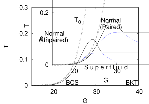
Figure 1: Phase diagram of temperature $T$ (in units of $\epsilon_{2D}$) versus $G=mAg/(4\pi)$ for a mixture of equal masses with s-wave interactions, interaction range $k_{0}\sim 10^{4}k_{2D}$, tunneling $t_{z}\approx 0.043\epsilon_{2D}$, lattice spacing $a_{z}\approx 0.43{\rm\mu m}$ and planar density $n_{2D}\approx 2.5\times 10^{7}{\rm cm^{-2}}$, such that $k_{2D}a_{z}\approx 2.2$. $T_{0}$ is the saddle-point or pairing temperature scale.

To recover the BKT physics in the $G\gg 1$ limit where the paired fermions live in 2D planes, we return to the derivation of the fluctuation action $S_{fl}$ with $t_{z,\sigma}=0$. Taking the order parameter as $\Phi(x)=[|\Delta_{0}|+|\eta(x)|]e^{i\theta(x)},$ where $|\eta(x)|$ corresponds to the amplitude fluctuations and $\theta(x)$ is the phase of the order parameter such that $|\Delta_{0}|\gg|\eta(x)|$, we obtain the phase-only action $S_{fl}(\theta)=(\beta/2)\sum_{q}\left[\kappa_{0}(T)v_{\ell}^{2}+q_{i}\rho_{i,j}(T)q_{j}\right]\theta(q)\theta(-q).$ Here, the coefficient $\kappa_{0}(T)=(1/4)\sum_{\mathbf{k}}[|\Delta_{\mathbf{k}}|^{2}{\cal X}_{\mathbf{k},+}/E_{\mathbf{k},+}^{3}+\beta\xi_{\mathbf{k},+}^{2}{\cal Y}_{\mathbf{k},+}/(2E_{\mathbf{k},+}^{2})]$ is the atomic compressibility, where ${\cal Y}_{\mathbf{k},\pm}=({\cal Y}_{\mathbf{k},1}\pm{\cal Y}_{\mathbf{k},2})/2$ with ${\cal Y}_{\mathbf{k},s}={\rm sech}^{2}(\beta E_{\mathbf{k},s}/2)$; while the coefficient of the gradient term

$$\rho_{ij}(T) = \frac{n\delta_{ij}}{4m_{+}}-\sum_{\mathbf{k}}\frac{k_{i}k_{j}}{16A}\bigg{\{}\frac{4|\Delta_{\mathbf{k}}|^{2}}{m_{-}^{2}}\left(\frac{{\cal X}_{\mathbf{k},+}}{E_{\mathbf{k},+}^{3}}-\frac{\beta{\cal Y}_{\mathbf{k},+}}{2E_{\mathbf{k},+}^{2}}\right)$$ (10)

$$+ \beta\left[\frac{{\cal Y}_{\mathbf{k},1}}{m_{\uparrow}^{2}}+\frac{{\cal Y}_{\mathbf{k},2}}{m_{\downarrow}^{2}}-\frac{4{\cal Y}_{\mathbf{k},-}}{m_{+}m_{-}}\left(1-\frac{\xi_{\mathbf{k},+}}{E_{\mathbf{k},+}}\right)\right]\bigg{\}}$$

is the phase stiffness, where $\rho_{ij}(T)=\rho_{0}(T)\delta_{ij}$ for the s-wave symmetry.

This leads to the BKT transition temperature berezinskii-1971 ; kosterlitz-1972

$$T_{BKT}=\pi\rho_{0}(T_{BKT})/2,$$ (11)

which needs to be solved self-consistently with Eqs. (4) and (6) in order to determine $T_{BKT}$, $|\Delta_{0}|$ and $\mu_{\sigma}$ as a function of $G$. In the weak attraction regime ($G\lesssim 1$), $T_{BKT}$ increases with $G$ as $T_{BKT}=(e^{\gamma}/\pi)(2|\epsilon_{b}|\epsilon_{2D})^{1/2},$ where $\gamma\approx 0.577$ is the Euler’s constant and $\epsilon_{b}=-2\epsilon_{0}\exp(-1/G)$ is the binding energy in 2D. While in the strong attraction regime ($G\gg 1$), $T_{BKT}$ saturates to $T_{BKT}=(\epsilon_{2D}/8)[1-2m_{+}^{2}/(3m_{-}^{2})].$ For equal mass mixtures ($m_{-}\to\infty$), this reduces to $T_{BKT}=0.125\epsilon_{F}$ which can be seen in Fig. 1. Here, $\epsilon_{F}\equiv\epsilon_{2D}$ is the 2D Fermi energy.

To estimate when $G$ induces the crossover from anisotropic-3D to 2D behavior, we compare the critical temperature $T_{c,Gauss}$ obtained from the Gaussian theory with the critical temperature $T_{BKT}$ for the BKT transition in the strict 2D limit. When $G\gg 1$, the condition $T_{c,Gauss}=T_{BKT}$ leads to

$$t_{z,c,\uparrow}t_{z,c,\downarrow}=\frac{\zeta^{2}(3/2)}{2^{12}\pi}\left(\frac{m_{B}}{m_{+}}\right)^{2}\left(1-\frac{2m_{+}^{2}}{3m_{-}^{2}}\right)^{3}\epsilon_{2D}|\epsilon_{b}|,$$ (12)

where $\zeta(x)$ is the zeta function. This relation reduces to $t_{z,c}=\left[\zeta(3/2)/(32\sqrt{\pi})\right](\epsilon_{2D}|\epsilon_{b}|)^{1/2}$ for mixtures of equal mass fermions and equal tunneling.

We can also relate $t_{z,\sigma}$ to the depth $V_{0,\sigma}$ of the 1D optical latttice potential $V_{\sigma}(\mathbf{r})=V_{0,\sigma}\sin^{2}(\pi z/a_{z})$ where $t_{z,\sigma}=(2E_{r,\sigma}/\sqrt{\pi})(\alpha_{\sigma})^{3/4}\exp(-2\sqrt{\alpha_{\sigma}}).$ Here, $\alpha_{\sigma}=V_{0,\sigma}/E_{r,\sigma}$ where $E_{r,\sigma}=\pi^{2}/(2m_{\sigma}a_{z}^{2})$ is the recoil energy. In Fig. 2, we show the characteristic $t_{z,c}=t_{z,c,\sigma}$ and $V_{0,c}=V_{0,c,\sigma}$ lines which separate the anisotropic-3D from the 2D regime, for mixtures of equal mass, equal tunneling and s-wave interactions. When $G$ is fixed, the 2D regime may be reached from the anisotropic-3D regime with increasing $V_{0}=V_{0,\sigma}$ or decreasing $t_{z}=t_{z,\sigma}$. While for fixed $V_{0}=V_{0,\sigma}$ or $t_{z}=t_{z,\sigma}$, the 2D regime may be reached from the anisotropic-3D regime by increasing $G$.

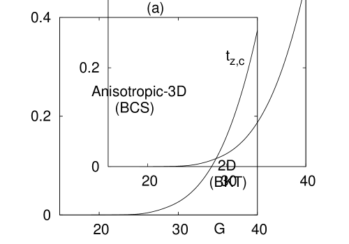
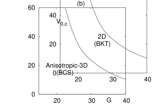
Figure 2: Characteristic (a) tunneling amplitude $t_{z,c}$ (in units of $\epsilon_{2D}$); and (b) optical lattice depth $V_{0,c}$ (in units of $E_{r}$) versus $G=mAg/(4\pi)$ showing the anisotropic-3D to 2D crossover. The parameters are the same as in Fig. 1.

Further insight into the dimensional crossover is gained by rewriting $S_{fl}$ with $t_{z,\sigma}\neq 0$ in real space and time such that $S_{fl}(\lambda^{*},\lambda)=(1/V)\int dtdr_{\perp}dz{\cal L}_{fl}(\lambda^{*},\lambda),$ where ${\cal L}_{fl}(\lambda^{*},\lambda)=\lambda^{*}(x)({\cal O}-c_{z}\partial_{z}^{2})\lambda(x)+b|\lambda(x)|^{4}/2$ is the Lagrangian. Here, $V$ is the volume, $\lambda(x)\equiv\lambda(r_{\perp},z,t)$ is the fluctuation field and ${\cal O}=a-c_{\perp}\nabla_{\perp}^{2}-id\partial_{t}.$ Upon discretization $z=na_{z}$, $S_{fl}$ reduces to the Lawrence-Doniach (LD) action $S_{LD}(\lambda_{n}^{*},\lambda_{n})=[1/(MA)]\sum_{n}\int dtdr_{\perp}{\cal L}_{LD}(\lambda_{n}^{*},\lambda_{n}),$ where

$${\cal L}_{LD}(\lambda_{n}^{*},\lambda_{n})=\lambda_{n}^{*}{\cal O}\lambda_{n}+\frac{c_{z}}{a_{z}^{2}}|\lambda_{n+1}-\lambda_{n}|^{2}+\frac{b}{2}|\lambda_{n}|^{4}$$ (13)

is the LD Lagrangian lawrence-doniach-1971 . Here, the local field $\lambda_{n}\equiv\lambda(r_{\perp},z=na_{z},t)$ describes the order parameter in each plane labeled by index $n$. Writing $a=a_{0}\epsilon(T)$ with $\epsilon(T)=(T-T_{c})/T_{c},$ scaling the field $\psi_{n}=\sqrt{b/a_{0}}\lambda_{n}$, and defining the correlation lengths $\xi_{0,\perp}^{2}=c_{\perp}/a_{0}$ and $\xi_{0,z}^{2}=c_{z}/a_{0}$, and the characteristic time $\tau_{0}=-d/a_{0}$ leads to the scaled action $\widetilde{\cal L}_{LD}(\psi_{n}^{*},\psi_{n})=\psi_{n}^{*}i\tau_{0}\partial_{t}\psi_{n}+\epsilon(T)|\psi_{n}|^{2}+\xi_{0,\perp}^{2}|\nabla_{\perp}\psi_{n}|^{2}+\xi_{0,z}^{2}|\psi_{n+1}-\psi_{n}|^{2}/a_{z}^{2}+|\psi_{n}|^{4}/2$, which describes the system near $T_{c}$. Here, $\widetilde{\cal L}_{LD}(\psi_{n}^{*},\psi_{n})=(b/a_{0}^{2}){\cal L}_{LD}(\lambda_{n}^{*},\lambda_{n}).$ Furthermore, taking $\psi_{n}=|\psi_{n}|\exp(i\theta_{n})$ in the LD action, such that $|\psi_{n}|=\phi_{0}$ is independent of position and time, leads to the phase-only anisotropic-3D XY model with the dimensionless Hamiltonian

$$\widetilde{H}_{XY}(r_{\perp},n)=K_{\perp}|a_{\perp}\nabla_{\perp}\theta_{n}|^{2}-2K_{z}\cos(\theta_{n+1}-\theta_{n})+C,$$

where $K_{\perp}=(\xi_{0,\perp}\phi_{0}/a_{\perp})^{2}$, $K_{z}=(\xi_{0,z}\phi_{0}/a_{z})^{2}$ and $a_{\perp}\sim k_{2D}^{-1}$, and $C$ is a constant. The dimension-full Hamiltonian is $\widetilde{H}_{XY}(r_{\perp},n)=(b/a_{0}^{2})H_{XY}(r_{\perp},n).$

This can be mapped into the vortex-loop representation shenoy-1995 yielding the dual dimensionless Hamiltonian

$$\widetilde{H}_{D}=\pi\sum_{\mathbf{r}\neq\mathbf{r^{\prime}}}[K_{z}J_{\perp}(\mathbf{r})\cdot J_{\perp}(\mathbf{r^{\prime}})+K_{\perp}J_{z}(\mathbf{r})\cdot J_{z}(\mathbf{r^{\prime}})]U(\mathbf{R}),$$

where $U(\mathbf{R}=\mathbf{r}-\mathbf{r^{\prime}})$ plays the role of an interaction potential for the vortex loop field $\mathbf{J}(\mathbf{r})=[J_{\perp}(\mathbf{r}),J_{z}(\mathbf{r})],$ and satisfies the differential equation $(\nabla_{\perp}^{2}+\eta^{-2}\partial_{z}^{2})U(\mathbf{R})=-4\pi\delta(\mathbf{R}).$ Here, $\eta=\sqrt{K_{\perp}/K_{z}}$ is the anisotropy ratio and $\delta(x)$ is the delta function. The dual transformation maps closed supercurrent flows associated with the gradients of the phase $\theta$ into the vortex-loop vector $\mathbf{J}(\mathbf{r})$, in the same way that the electric current flowing on a ring can be mapped into a magnetic field vector with the help of the Biot-Savart law.

For large magnitudes of $\mathbf{R}=(R_{\perp},R_{z})$, the vortex-loop interaction behaves asymptotically as $U(\mathbf{R})\sim 1/\sqrt{[R_{\perp}/(\eta a_{\perp})]^{2}+(R_{z}/a_{z})^{2}},$ and leads to equipotentials in the shape of ellipsoids $[R_{\perp}/(\eta a_{\perp})]^{2}+(R_{z}/a_{z})^{2}=U_{0}^{-2}$ when $U(\mathbf{R})=U_{0}$. Elliptical vortex loops corresponding to a nearly toroidal arrangement of the supercurrent flow are the large scale excitations formed by a continuous closed line having the same potential between segments with $\mathbf{r}=-\mathbf{r^{\prime}}$. When $\eta\to\infty$, the planes along the $\mathbf{z}$ direction decouple (2D BKT regime) and the vortex loops reduce to planar vortex-antivortex pairs. For $2<\eta<\infty$, the system is still nearly 2D, and the dominant excitations are square vortex loops coupling two consecutive planes and planar vortex loops. However, in the anisotropic-3D regime when $\eta<2$, the dominant excitations become multiplane elliptical vortex loops.

In the strong attraction regime $(G\gg 1)$, $\eta\approx(a_{z}/a_{\perp})\sqrt{m_{B,z}/m_{B,\perp}}\gg 1,$ and the 2D BKT limit is recovered since $m_{B,z}\gg m_{B,\perp}$. For fermion mixtures of equal masses and equal tunnelings, we can rewrite this condition as $\eta\approx\sqrt{\epsilon_{2D}|\epsilon_{b}|}/(4\pi t_{z})\gg 1.$ Since the anisotropic-3D to 2D crossover occurs for $\eta\approx 2$, this condition leads to $t_{z,c}\approx(1/8\pi)(\epsilon_{2D}|\epsilon_{b}|)^{1/2}$, which is essentially the same result obtained by equating the Gaussian and BKT critical temperatures.

Vortex-antivortex pairs have been detected in ultracold atoms using absorption images of an expanding cloud helmerson-2008 , and we expect that similar techniques can be used to detect vortex loops as the system evolves from anisotropic-3D to 2D regime. Vortex loops should appear as dark rings in the image since there are no atoms to absorb light in their cores. At temperature $T$, the ratio of characteristic in situ core size of vortex loops in the $(x,y)$ plane $\xi_{\perp}(T)=\xi_{0,\perp}|\epsilon(T)|^{-2/3}$ and along the $\mathbf{z}$ direction $\xi_{z}(T)=\xi_{0,z}|\epsilon(T)|^{-2/3}$ is $\xi_{\perp}(T)/\xi_{z}(T)\approx 0.91$ for $\eta=2$ and $k_{2D}a_{z}=2.2$. Since typical values of $\xi_{0,\perp}\approx 0.5{\rm\mu m}$, then $\xi_{\perp}(T)\approx 2.3{\rm\mu m}$ and $\xi_{z}(T)\approx 2.5{\rm\mu m}$ at temperatures $T=0.9T_{c}$, and vortex loops extend to nearly six planes for an optical lattice with $a_{z}\approx 0.43{\rm\mu m}$. Smaller values of $\eta$ or larger values of $k_{2D}a_{z}$ enlarge $\xi_{z}(T)$. For parameters $\eta=1.7$, $k_{2D}a_{z}=5.0$ and $T=0.9T_{c}$, the ratio $\xi_{\perp}(T)/\xi_{z}(T)\approx 0.34$ and $\xi_{z}(T)\approx 6.8{\rm\mu m}$, such that vortex loops extend to nearly sixteen planes in optical lattices with $a_{z}\approx 0.43{\rm\mu m}$.

We analyzed the finite temperature phase diagram of attractive fermion mixtures in 1D optical lattices. At low temperatures, we found that a dimensional crossover from an anisotropic-3D (BCS) to an effectively 2D (BKT) superfluid occurs as a function of attraction strength eventhough the tunneling amplitude is fixed. In addition, we discussed that vortex excitations change from elliptical multiplane vortex loops in the anisotropic-3D regime to planar vortex-antivortex pairs in the 2D regime, and suggested an experiment to detect their presence.

We thank the NSF (DMR-0709584) for support.

References

• (1) I. Bloch, Nature Phys. 1, 23 (2005).
• (2) J. K. Chin et al., Nature (London) 443, 961 (2006).
• (3) V. L. Berezinskii, Sov. Phys. JETP 32, 493 (1971).
• (4) J. M. Kosterlitz and D. Thouless, J. Phys. C 5, L124 (1972).
• (5) Z. Hadzibabic et al., Nature 441, 1118 (2006).
• (6) T. Stöferle et al., Phys. Rev. Lett. 96, 030401 (2006).
• (7) S. Ospelkaus et al., Phys. Rev. Lett. 97, 120403 (2006).
• (8) M. Iskin and C. A. R. Sá de Melo, Phys. Rev. Lett. 99, 080403 (2007).
• (9) H. Zhai ad T.-L. Ho, Phys. Rev. Lett. 99 100402 (2007).
• (10) E. G. Moon et al., Phys. Rev. Lett. 99 230403 (2007).
• (11) C. A. R. Sá de Melo et al., Phys. Rev. Lett. 71, 3202 (1993).
• (12) W. E. Lawrence and S. Doniach, in Proc. $12^{th}$ Int. Conf. Low. Temp. Phys., p. 361, E. Kanda (ed.), Tokyo (1971).
• (13) S. R. Shenoy, and B. Chattopadhyay, Phys. Rev. B 51, 9129 (1995).
• (14) Kristian Helmerson, private communication (2008).