Adiabatic cavity QED with pairs of atoms

Abstract

We study the dynamics of a pair of atoms, resonantly interacting with a single mode cavity, in the situation where the atoms enter the cavity with a time delay between them. Using time dependent coupling functions to represent the spatial profile of the mode, we considered the adiabatic limit of the system. Although the time evolution is mostly adiabatic, energy crossings play an important role in the system dynamics. Following from this, entanglement, and a procedure for cavity state teleportation are considered. We examine the behaviour of the system when we introduce decoherence, a finite detuning, and potential asymmetries in the coupling profiles of the atoms.

1 Introduction

Entanglement between Quantum systems is important for the realisation of a Quantum Computer Nielsen . In recent years many authors have proposed different methods, based on cavity QED systems, for entangling atoms. Some of these proposals use single resonant interactions Zheng2005 or strongly detuned cavities Zheng2000 ; Jane2002 ; You2003b , or the adiabatic sequential passage of atoms through cavities Marr2003 ; Yong2007 . Other schemes use decoherence-free spaces and continuous monitoring of the cavity decay for generating entangled states Plenio1999 ; Beige2000a ; Beige2000b . Another approach is to make use of photon polarisation measurements for characterising the final atomic state Shorencen2003 ; Chen2003 ; Duan2003 .

In a recent work Lazarou2007 , we considered an entangling system consisting of a pair of two-level atoms resonantly interacting with a single mode cavity. Taking into account the sequential motion of the atoms through the cavity and the spatial profile of the mode, we utilised an atom-cavity interaction with identical time dependent coupling functions for both atoms. The main feature for this resonant system, when considering the adiabatic limit, was the existence of an energy crossing at the vicinity of a temporal degeneracy. Furthermore, one of the atoms entangles to the cavity, and the system evolution for large photon numbers has a resemblance to the Jaynes-Cummings model. Based on these features, fairly robust methods for entangling the atoms, for quantum state mapping and implementing a SWAP and a C-NOT gate were proposed.

Here we examine the system dynamics in a more general approach by considering the possibility of a finite detuning between a the atoms and the cavity mode, and the potential of having asymmetries in the coupling profiles of the two atoms with respect to each other. Furthermore, we also study the role of decoherence and how this affects the dynamics, but also the fidelity of the proposed applications. As long as the detuning is relatively small, the system behaves in a similar way as before. The atom that enters the cavity second becomes entangled with the field mode, whereas the first atom does not. Furthermore one can still map this entanglement onto the pair of atoms. As long as the detuning is small the fidelity is relatively high.

On the other hand, for increasing values of the detuning various non-adiabatic effects related to avoided crossings in the adiabatic spectrum, give rise to a tri-partite entanglement between the cavity and both atoms. For detuning much larger than the coupling strength, the cavity is disentangled from the system with the atoms being entangled to each other, while the cavity is only virtually excited Yong2007 .

The differences between the coupling functions for the two atoms, give rise to somewhat different dynamics. Although the second atom still entangles to the cavity, there are two paths which depend on the initial state of the second atom. The system is then characterised by two mixing angles which are functions of the coupling, the interaction time, the photon number and the asymmetry factor of the two coupling profiles.

For a leaky cavity, the effects on the fidelity of the system, and generally the system dynamics, are suppressed as long as a high $Q$ cavity is being used. For example micromaser cavities with $Q\sim 10^{10}$ could be used to experimentally realise the proposed model with negligible effects on the system.

In the following section we introduce the model and the corresponding Hamiltonian, discuss in brief the resonant limit and propose a teleportation protocol for field state transfer between cavities. In section 3, a detailed analysis for the case of asymmetric atomic coupling profiles is presented. Furthermore we discuss the off-resonant limit, and in section 4 we discuss decoherence effects and how these affect the system. Finally in section 5 we conclude by summarising our results.

2 The atom-cavity model

2.1 The Hamiltonian

In our model a pair of two-level atoms enters a single mode cavity at different times, moving along the $x$ axis, atom 1, and parallel to this, atom 2, figure 1. The field spatial profile has the form of a Gaussian function along the $x$ direction with additional spatial modulation along the $y$ direction

$$E(x,y)=E_{0}(y)\exp\big{(}-\frac{x^{2}}{4x_{0}^{2}}\big{)}.$$ (1)

Replacing the displacement operator with its classical counterpart, $\hat{x}_{j}(t)\rightarrow v_{j}t$, we get the following coupling functions, or profiles, for the two atoms

$$\eta_{\scriptscriptstyle 1}(\tau)=g_{1}e^{-(\tau+\delta)^{2}},\qquad\eta_{\scriptscriptstyle 2}(\tau)=g_{2}e^{-(\tau-\delta)^{2}}.$$ (2)

The dimensionless time $\tau$ and the parameter $\delta$ are defined in terms of the time width $\sigma=x_{0}/v$

$$\tau=\frac{t}{2\sigma},\qquad\delta=\frac{\Delta t}{2\sigma}.$$ (3)

The time interval $\Delta t$ is the time delay after which atom 2 enters the cavity and $v$ the velocity of the atoms which is taken to be the same for both atoms. We have already seen in Ref. Lazarou2007 , that the resonant non-dissipative system is not too sensitive to the delay time $\delta$ and we will rely on this in what follows.

Since atom 1 is moving along axis $x$ and atom 2 along a displaced trajectory, figure 1, and because the field strength depends on $y$ the coupling for the second atom will be modified by a factor $\epsilon$ with respect to $g_{1}=g_{0}$, $g_{2}=\epsilon g_{1}$. The parameter $\epsilon$ is the asymmetry factor for the coupling profiles.

For the Eq. (3) to be valid the two atoms must be moving sufficiently fast so that they don’t get reflected by the cavity. This means that the atomic velocity $v$ must be mush greater than the barrier set by the maximum coupling strength $g_{0}$, $v\gg\sqrt{2\hbar g_{0}/m}$, where $m$ is the atomic mass. Then, if this is the case the centre of mass motion is considered to be classical and one can make the substitution $\hat{x}_{j}(t)\rightarrow vt$.

In the interaction picture, and within the rotating wave approximation, the Hamiltonian reads $(\hbar=1)$

$$H_{I}(t)=\Delta\left(|e_{1}e_{2}\rangle\langle e_{1}e_{2}|-|g_{1}g_{2}\rangle\langle g_{1}g_{2}|\right)+\sum_{j=1}^{2}\eta_{j}(t)\big{(}a^{\dagger}\sigma^{j}_{-}+a\sigma^{j}_{+}\big{)}.$$ (4)

The operators $a^{\dagger}$ and $a$ are the Bosonic creation-annihilation operators for the cavity mode, and $\sigma^{j}_{-}$ and $\sigma^{j}_{+}$ are the lowering-raising operators for atom $j$. The detuning between the atomic transition and the mode frequency is $\Delta$. The ground state for atom $j$ is $|g_{j}\rangle$ and the corresponding excited is $|e_{j}\rangle$.

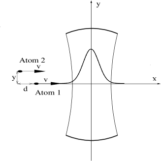
Figure 1: The experimental setup: Two identical two-level atoms enter a single mode cavity along two different trajectories. Both atoms are moving with the same velocity, but they enter and exit the cavity at different times. The field inside the cavity has a Gaussian profile along the $x$ axis.

2.2 Resonant limit

In a previous work Lazarou2007 , we considered the adiabatic limit for the Hamiltonian (4) with $\Delta=0$, and emphasis in the case of equal coupling amplitudes $g_{1}=g_{2}=g_{0}$, although some of the results are somewhat more general and apply in the case of different couplings $g_{1}\neq g_{2}$.

In the adiabatic limit one can diagonalise the Hamiltonian assuming that the time is a parameter to obtain the time dependent adiabatic energies and the corresponding state vectors Messiah . The only relevant bare states for the purposes of our analysis are those with the same number of total excitations since the total number of excitations is a constant of motion

$$|n,e_{1}e_{2}\rangle,\quad|n+1,g_{1}e_{2}\rangle,\quad|n+1,e_{1}g_{1}\rangle,\quad|n+2,g_{1}g_{2}\rangle.$$ (5)

After diagonalising the Hamiltonian (4), we get the following adiabatic energies and the corresponding state vectors Lazarou2007 ; Mahmood1987

$$E_{1,2}(\tau) =\mp E_{-}(\tau),\qquad E_{3,4}=\mp E_{+}(\tau),$$ (6a)

$$E_{\pm}(\tau) =\sqrt{\frac{(3+2n)(\eta_{\scriptscriptstyle 1}^{2}(\tau)+\eta_{\scriptscriptstyle 2}^{2}(\tau))\pm F_{n}(\tau)}{2}},$$ (6b)

where the function $F_{n}(\tau)$ is

$$F_{n}(\tau)=\sqrt{\big{(}\eta_{\scriptscriptstyle 1}^{2}(\tau)+\eta_{\scriptscriptstyle 2}^{2}(\tau)\big{)}^{2}+16(n+1)(n+2)\eta_{\scriptscriptstyle 1}^{2}(\tau)\eta_{\scriptscriptstyle 2}^{2}(\tau)}.$$ (7)

and

$$\left|\Psi_{1,2}(\tau)\right\rangle= A_{-}(\tau)|n,e_{1}e_{2}\rangle+D_{-}(\tau)|n+2,g_{1}g_{2}\rangle$$

$$\pm\big{(}B_{-}(\tau)|n+1,g_{1}e_{2}\rangle-C_{-}(\tau)|n+1,e_{1}g_{2}\rangle\big{)},$$ (8a)

$$\left|\Psi_{3,4}(\tau)\right\rangle= A_{+}(\tau)|n,e_{1}e_{2}\rangle+D_{+}(\tau)|n+2,g_{1}g_{2}\rangle$$

$$\pm\big{(}B_{+}(\tau)|n+1,g_{1}e_{2}\rangle-C_{+}(\tau)|n+1,e_{1}g_{2}\rangle\big{)}.$$ (8b)

The upper sign in Eqs. (8) is for the odd numbered states and the lower one is for the even ones.

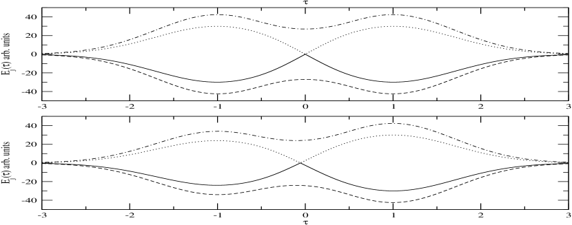
Figure 2: The adiabatic energies. Top: The symmetric limit $\epsilon=g_{1}/g_{2}=1.0$. Bottom: The asymmetric case for $\epsilon=0.8$. The energies are $E_{1}(\tau)$ (solid), $E_{2}(\tau)$ (dot), $E_{3}(\tau)$ (dashed) and $E_{4}(\tau)$ (dot-dashed). The other parameters are: $\delta=1.0$, $n=0$ and $\Delta=0$.

A first important property for the adiabatic states is the temporal degeneracy for two of them, figure 2. From Eq. (6a) we can see that for $\eta_{1}(t)=\eta_{2}(t)$ we have that $E_{1}(t)=E_{2}(t)$. When $g_{1}=g_{2}$ then $t=0$ and for $g_{1}\neq g_{2}$ then $t$ has a finite value at the degeneracy which is a function of the ratio $\epsilon=g_{2}/g_{1}$.

In the vicinity of this temporal degeneracy the adiabatic approximation will fail and this is because the adiabatic theorem holds only for non-degenerate states Messiah . One can show that near this point the system undergoes a pure crossing even for unequal couplings $g_{1}\neq g_{2}$. The reason for this behaviour is the diagonal form that the Hamiltonian has in the vicinity of the temporal degeneracy, and the fact that the two adiabatic states, $\left|\Psi_{1}\right\rangle$ and $\left|\Psi_{2}\right\rangle$, do not couple near the crossing. Thus, if the system is initially in state $\left|\Psi_{1}(-\infty)\right\rangle$, $\left(\left|\Psi_{2}(-\infty)\right\rangle\right)$, then for $t\rightarrow\infty$ the final state will be $\left|\Psi_{2}(\infty)\right\rangle$, $\left(\left|\Psi_{1}(\infty)\right\rangle\right)$ with an arbitrary phase factor $\theta_{n}$, i.e.

$$\left|\Psi_{1}(-\infty)\right\rangle\rightarrow e^{-\dot{\imath}\theta_{n}}\left|\Psi_{2}(\infty)\right\rangle,\quad\left|\Psi_{2}(-\infty)\right\rangle\rightarrow e^{\dot{\imath}\theta_{n}}\left|\Psi_{1}(\infty)\right\rangle,$$ (9)

and

$$\theta_{n}=\int_{-\infty}^{0}d\tau^{\prime}E_{1}(\tau^{\prime})+\int_{0}^{\infty}d\tau^{\prime}E_{2}(\tau^{\prime}).$$ (10)

2.3 Input-output in terms of the bare states for $\Delta=0$

For equal couplings $\epsilon=1$, then $\theta_{n}=0$. For this limit, and with the following relations for the coupling functions Eq. (2)

$$\lim_{\tau\rightarrow\infty}\left(\frac{\eta_{\scriptscriptstyle 1}}{\eta_{\scriptscriptstyle 2}}\right)=0,\qquad\lim_{\tau\rightarrow-\infty}\left(\frac{\eta_{\scriptscriptstyle 2}}{\eta_{\scriptscriptstyle 1}}\right)=0,$$ (11)

the following input-output table in terms of the bare states (5) is obtained

$$|n,e_{1}e_{2}\rangle\rightarrow|n,e_{1}e_{2}\rangle,$$ (12a)

$$|n+1,g_{1}e_{2}\rangle\rightarrow-|n+1,e_{1}g_{2}\rangle,$$ (12b)

$$|n+1,e_{1}g_{2}\rangle\rightarrow\cos(\phi_{n})|n+1,g_{1}e_{2}\rangle-\dot{\imath}\sin(\phi_{n})|n+2,g_{1}g_{2}\rangle,$$ (12c)

$$|n+2,g_{1}g_{2}\rangle\rightarrow\cos(\phi_{n})|n+2,g_{1}g_{2}\rangle-\dot{\imath}\sin(\phi_{n})|n+1,g_{1}e_{2}\rangle,$$ (12d)

where the angle $\phi_{n}$ reads

$$\phi_{n}=\phi_{4}(\infty)=-\phi_{3}(\infty)=\int_{-\infty}^{\infty}d\tau E_{4}(\tau).$$ (13)

Equation (12b) describes a complete energy transfer between the two atoms. This will happen without choosing special values for the system parameters provided we ensure the necessary conditions for adiabatic evolution. This robust energy transfer is a reminiscent of the STIRAP method Bergmann1998 ; Bergmann1995 . We also note that Eqs. (12c) and (12d) describe a conditional entanglement of the second atom to the field mode. If atom 2 is not excited, then it will be entangled to the field mode.

An interesting limit for $\phi_{n}$ is the one for $n\gg 1$. In this limit one can show that $\phi_{n}$ has the same dependence with respect to $n$ as the mixing angle in the Jaynes-Cummings model Lazarou2007 : $\phi_{n}\approx 4g\sigma\sqrt{n\pi}$ for $n\gg 1$. This result suggests that for a large number of photons and with adiabatic evolution, we will have the same kind of dynamics as in the usual single atom Jaynes-Cummings model. What is different is that this Jaynes-Cummings rotation is conditional upon the state of the second atom. This could used for conditional operations in quantum information or for preparing field states with the use of conditional control. Of course in this limit the field dynamics will be the same as for the Jaynes-Cummings model Scully .

2.4 Applications: Quantum teleportation between cavities

Based on this input-output table applications in the field of Quantum Information and Quantum teleportation can be realised. We have discussed the implementation of SWAP and C-NOT gates, generating atomic entanglement and robust quantum state mapping. The proposed applications are fairly robust and rely on the control of a single parameter, i.e. the mixing angle $\phi_{n}$. Furthermore the proposed applications are characterised by relatively high fidelities up to $99\%$ even for errors of the order of $10\%$ in $\delta$ or $1\%$ in $\sigma$ Lazarou2007 .

To this end is interesting to consider in detail the realisation of a teleportation protocol between two different cavities. The setup consists of three identical cavities placed in a row, with classical EM fields between them. Assuming that the first cavity is initially in the superposition

$$\alpha|0\rangle+\beta|1\rangle,$$

we send a pair of non-excited atoms through the first cavity, ensuring that $\phi_{-1}=\pi/2$. Then according to Eqs.(12) , the state of atom 2 will be

$$\alpha|g_{2}\rangle-\dot{\imath}\beta|e_{2}\rangle.$$

Using the EM field after cavity 1 we perform the phase transformation $|e_{2}\rangle\rightarrow\dot{\imath}|e_{2}\rangle$. In this way the mode state for cavity 1 is mapped onto atom 2, while atom 1 and cavity 1 are not excited.

The atoms now cross the second (auxiliary) cavity with arbitrary $\phi_{-1}$. Subsequently we perform a rotation $-\dot{\imath}|e_{1}\rangle$ with an EM field so that we get the state

$$|0;g_{2}\rangle\left(\alpha|g_{1}\rangle+\dot{\imath}\beta|e_{1}\rangle\right).$$

Finally, the two atoms cross the third cavity with $\phi_{-1}=\pi/2$; the result is to get both atoms in their ground state and the cavity 3 in the same state as cavity 1 was initially. Thus with this fairly simple method we can teleport the state of a cavity to another cavity.

For the results up to this point, and for the proposed applications to be valid the adiabatic approximation must hold. This will be true as long as the coupling strength is greater than a lower bound defined by the interaction time and the photon number $n$. For small photon numbers, $n\sim 1$, the coupling strength must be of the order of $10/\sigma$. For a larger number of excitations in the cavity, this lower bound increases meaning that the coupling strength or the interaction time must also increase for the adiabatic approximation to be valid Lazarou2007 . In addition the delay time $\Delta t$ must be of the order of the interaction time. Furthermore, the system is fairly robust with respect to this parameter, since in our scheme the accurate control of $\delta$ is not important. Instead a rather simple condition with $\delta\sim 1$, i. e. $1.0\leq\delta\leq 1.25$, must be satisfied as seen in Ref. Lazarou2007 .

3 Effects due to different couplings and finite detuning

3.1 Different couplings

As already mentioned in section 2.2 the results for the adiabatic states and the corresponding energies are general and hold even if $\epsilon\neq 1$. The energy crossing will exist for $g_{1}\neq g_{2}$ but the point where this occurs is no longer at $t=0$. Because of this the mixing angle $\theta_{n}$ is no longer zero since the energies $E_{1}(\tau)$ and $E_{2}(\tau)$ are no longer symmetrical; i.e. $E_{j}(-\tau)\neq E_{j}(\tau),\quad j=1,2$ although $E_{1}(\tau)=-E_{2}(\tau)$, figure 2. Thus the integral (10) has a finite value. This results in input-output relations that differ from the ones in Eqs. (12).

For example, the state $|n;e_{1},e_{2}\rangle$ is equivalent to the following superposition for $\tau\rightarrow-\infty$

$$-\frac{\left|\Psi_{1}(\tau)\right\rangle+\left|\Psi_{2}(\tau)\right\rangle}{\sqrt{2}}.$$ (14)

For $\tau\rightarrow\infty$ and taking into account the crossing Eq. (9) we have

$$|n;e_{1},e_{2}\rangle\rightarrow-\frac{e^{\dot{\imath}\theta_{n}}\left|\Psi_{1}(\infty)\right\rangle+e^{-\dot{\imath}\theta_{n}}\left|\Psi_{2}(\infty)\right\rangle}{\sqrt{2}}.$$ (15)

Using the limits Eq. (11) and Eqs. (8) we have Lazarou2007

$$|n;e_{1},e_{2}\rangle\rightarrow\cos(\theta_{n})|n;e_{1},e_{2}\rangle-\dot{\imath}\sin(\theta_{n})|n+1;e_{1},g_{2}\rangle.$$ (16)

In a similar way we will find that

$$|n+1;g_{1},e_{2}\rangle\rightarrow\cos(\theta_{n})|n+1;e_{1},g_{2}\rangle-\dot{\imath}\sin(\theta_{n})|n+1;e_{1},e_{2}\rangle.$$ (17)

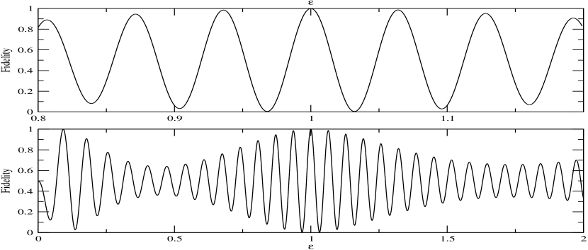
Figure 3: The fidelity for the maximally entangled state $\left|\Psi_{f}(0,2m\pi)\right\rangle$ Eq. (20), $\left|\left\langle\Psi_{f}(0,2m\pi)|\Psi_{f}(\theta_{0},\phi_{-1})\right\rangle\right|$ shown as a function of the asymmetry $\epsilon$. The parameters are: $\delta=1$, $\Delta=0$ and $g_{0}\sigma=28.3929$. The coupling $g_{0}$ was chosen so that for $\epsilon=1.0$ the fidelity is unity. The upper part of the figure expands the central region in the lower part of the figure.

In contrast to Eqs. (12a) and (12b), we see that there is no longer robust exchange of energy between the atoms. Furthermore, for $\epsilon\neq 1$ atom 2 will get entangled to the cavity mode without any condition on its initial state. If it is excited then the entanglement is defined by the mixing angle $\theta_{n}$, whereas if it is initially placed in its ground state the entanglement is defined by the mixing angle $\phi_{n}$. Both mixing angles have a dependence with respect to $\delta$, $n$, $\sigma$, $g_{0}$ and $\epsilon$. For $\theta_{n}=2\pi$ we recover the same input-output expressions as Eqs. (12).

An interesting feature of the system is that for $\epsilon\neq 1$, the robust state mapping between the two atoms, or the mapping between one of the atoms and the cavity, which depends on the mixing angle $\phi_{-1}$ and consequently the teleportation protocol in section 2.4 remains fairly robust. The reason for this is that for this application the only states involved are

$$|0;g_{1},e_{2}\rangle,\quad|0;e_{1},g_{2}\rangle,\quad|1;g_{1},g_{2}\rangle.$$ (18)

For this subspace the mixing angle $\theta_{n=-1}$ is zero by definition. Thus the only parameter to be controlled is the mixing angle, as in the case of identical coupling profiles, $\epsilon=1.0$.

On the other hand, applications, such as the entangling of atoms, become more involved since an extra control parameter, the angle $\theta_{n}$, appears in the system evolution. For example, if the initial state of the system is

$$\left|\Psi_{0}\right\rangle=\frac{1}{2}|0\rangle\left(|g_{1}\rangle+|e_{1}\rangle\right)\left(|g_{2}\rangle+|e_{2}\rangle\right),$$ (19)

then the output state will be

$$\left|\Psi_{f}(\theta_{0},\phi_{-1})\right\rangle = \frac{1}{2}\left(|g_{2}\rangle\left(|g_{1}\rangle-|e_{1}\rangle\right)+|e_{2}\rangle\left(\cos(\theta_{0})|e_{1}\rangle+\cos(\phi_{-1})|g_{1}\rangle\right)\right)$$ (20)

$$-\frac{\dot{\imath}}{2}\left(\sin(\theta_{0})|1;e_{1},g_{2}\rangle+\sin(\phi_{-1})|1;g_{1},g_{2}\rangle\right).$$

Thus, with a probability that always exceeds $50\%$ the two atoms are entangled to each other. For example if $\theta_{0}=2k\pi$ and $\phi_{-1}=2m\pi$, with $k$ and $m$ integers, the probability is one and the two atoms are maximally entangled. For different values of the mixing angles the probability is less than one and the entanglement is not maximal, and vanishes if $\cos(\theta_{0})=0=\cos(\phi_{-1})$.

Because of the complex dependence of both mixing angles with respect to the asymmetry $\epsilon$, the fidelity of a maximally entangled state is very sensitive with respect to $\epsilon$. For $\epsilon\sim 1$, it oscillates relatively fast with a decaying amplitude, figure 3, and revivals are observed for different values of the asymmetry parameter $\epsilon$. Despite this, and because the condition $\cos(\theta_{0})=0=\cos(\phi_{-1})$ is only satisfied for certain values of the asymmetry parameter, the atomic entanglement persists even if the asymmetry factor is not one.

3.2 Effects of the finite detuning

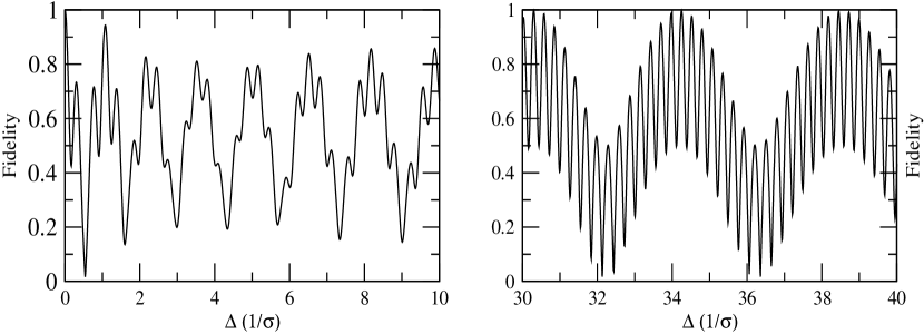
Figure 4: The fidelity for the maximally entangled state $\left|\Psi_{f}^{\Delta}(2m\pi,0)\right\rangle$ Eq. (26) with respect to the detuning $\Delta$. The result was obtained after numerical simulations with the Schrödinger equation for the time-dependent Hamiltonian (4). The integration interval is $-12\sigma\leq t\leq 12\sigma$, and the fidelity was calculated for $t=12\sigma$. The parameters are: $\delta=1.0$, $\epsilon=1.0$ and $g_{0}\sigma=28.3929$. For this coupling and for $\epsilon=1.0$ and $\Delta=0$ the fidelity is unity.

For finite detuning, one can show that the system has the following dark state

$$|D\rangle=\frac{1}{\sqrt{\eta_{1}^{2}+\eta_{2}^{2}}}\left(\eta_{1}|g_{1},e_{2}\rangle-\eta_{2}|e_{1},g_{2}\rangle\right)|0\rangle.$$ (21)

Taking into account Eq. (11) we see that the robust energy change between atoms, Eq. (12b), takes place even for a finite detuning. Thus the robust state mapping between the two atoms can be realised even if the detuning is not zero. Furthermore for $\Delta\gg g_{0}$, an effective Hamiltonian for the states $|0;g_{1},e_{2}\rangle$ and $|0;e_{1},g_{2}\rangle$ is obtained after adiabatic elimination of the off-resonant states $|0;e_{1},e_{2}\rangle$ and $|1;g_{1},g_{2}\rangle$.

This Hamiltonian has two eigenstates (adiabatic states), the dark state $|D\rangle$ Eq. (21), and

$$\left|\Psi\right\rangle=\frac{1}{\sqrt{\eta_{1}^{2}+\eta_{2}^{2}}}\left(\eta_{2}|g_{1},e_{2}\rangle+\eta_{1}|e_{1},g_{2}\rangle\right)|0\rangle,$$ (22)

where the corresponding adiabatic energy is

$$E_{\Psi}(t)=\frac{\eta_{1}^{2}+\eta_{2}^{2}}{\Delta}.$$ (23)

Taking into consideration Eq. (11) and Eqs. (21) and (22), we get the following input-output relations for the adiabatic limit

$$|g_{1},e_{2}\rangle\rightarrow-|e_{1},g_{2}\rangle,\quad|e_{1},g_{2}\rangle\rightarrow e^{-\dot{\imath}\Theta}|g_{1},e_{2}\rangle,$$ (24)

where the angle $\Theta$ reads

$$\Theta=\frac{2\sigma g_{0}^{2}}{\Delta}\int_{-\infty}^{\infty}E_{\Psi}(\tau)d\tau=\frac{2\sigma g_{0}^{2}(1+\epsilon^{2})}{\Delta}\sqrt{\frac{\pi}{2}}.$$ (25)

Equation (24) represents a SWAP operation, but when it is combined with the initial state $\left|\Psi_{0}\right\rangle$, Eq. (19), it gives the following output state

$$\left|\Psi_{f}^{\Delta}(\Theta,\Phi)\right\rangle=\frac{1}{2}|0\rangle\left(|g_{2}\rangle\left(|g_{1}\rangle-|e_{1}\rangle\right)+|e_{2}\rangle\left(e^{-\dot{\imath}\Theta}|g_{1}\rangle+e^{-\dot{\imath}\Phi}|e_{1}\rangle\right)\right).$$ (26)

The phase factor $e^{-\dot{\imath}\Phi}$ represents the phase acquired by the state $|0;e_{1},e_{2}\rangle$ during the system evolution. This is an entangled state of the two atoms and becomes a maximally entangled state if the two phases are both $e^{-\dot{\imath}\Theta}=e^{-\dot{\imath}\Phi}=\pm 1$ since the fidelity for the entangled state (26) is

$$F=\frac{1}{4}\left|2+e^{-\dot{\imath}\Theta}+e^{-\dot{\imath}\Phi}\right|,$$ (27)

and it has a maximum, $F=1$, for $\Theta=2m\pi$ and $\Phi=2k\pi$ where $m,k=\pm 1,\pm 2\dots$.

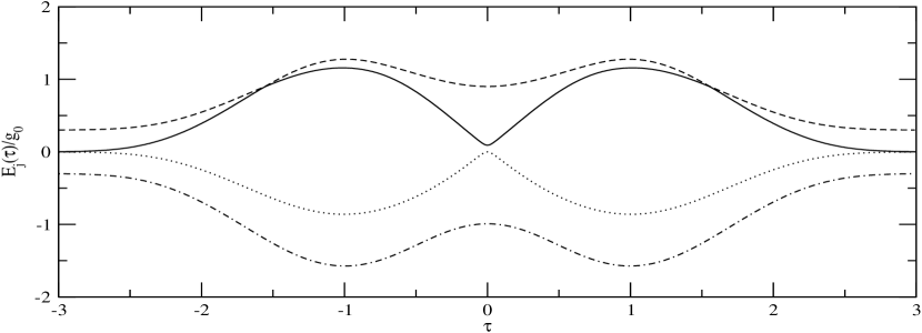
Figure 5: The adiabatic energies for $\Delta=15/\sigma$: $E_{1}(\tau)$ (dot), $E_{2}(\tau)$ (solid), $E_{3}(\tau)$ (dot-dashed) and $E_{4}(\tau)$ (dashed). The parameters are: $\delta=1.0$, $n=0$ and $\epsilon=1.0$. Notice the three avoided crossings for $\tau=0$ and the two symmetric with respect to $\tau=0$.

In figure 4, the fidelity is plotted with respect to the detuning $\Delta$ as calculated after numerically integrating the Schrödinger equation for the Hamiltonian (4). We see that for a small detuning the fidelity decays fast, below $50\%$, and then oscillates with a non harmonic profile, and an average value below unity, figure 4 (left). This is due to the fact that either both atoms, or one of them, entangles to the cavity, and thus we don’t have pure atomic entanglement. As the detuning increases the fidelity continues oscillating, but the average fidelity varies periodically between zero and one; figure 4 (right). Subsequent investigation has shown that these variations in the average fidelity are due to the interference between the two phase terms involving $e^{-\dot{\imath}\Phi}$ and $e^{-\dot{\imath}\Theta}$.

In general, the off-resonance case is characterised by three regimes. The first regime is that for small detuning, $\Delta/\sigma<20$, where the system qualitatively behaves in a similar way to the resonant case. More specifically the second atom entangles to the cavity mode, as is evidenced by the populations seen in figure 6. The entanglement depends on $\Delta$ and equations (12) are no longer valid.

For $\Delta\sim 20/\sigma$, the adiabatic spectrum has three avoided crossings, figure 5. Because of this the two atoms entangle to the cavity mode forming the state

$$c_{1}|n;e_{1},e_{2}\rangle+c_{2}|n+1;e_{1},g_{2}\rangle+c_{3}|n+1;g_{1},e_{2}\rangle.$$ (28)

Each of the three adiabatic states which are involved in the avoided crossings, figure 5, map, at $\tau\rightarrow\pm\infty$, with one of the three states appearing in Eq. (28). Because of the small gap in the vicinity of the avoided crossings, the three adiabatic states are coupled to each other and as a result the system, which starts in one of the three states, $|n;e_{1},e_{2}\rangle$, $|n+1;e_{1},g_{1}\rangle$ or $|n+1;g_{1},e_{2}\rangle$, ends up in an entangled state similar to (28), figure 6.

In the limit of large detuning, $\Delta\geq g_{0}$, as already discussed, the cavity is not excited and does not entangle to the atoms, as is shown by the populations seen figure 6. The two atoms can interact with each other via virtual excitations of the cavity field, and get entangled. Similar results were previously obtained for $\Delta\gg g_{0}$ with use of a time dependent Frölich transformation Yong2007 .

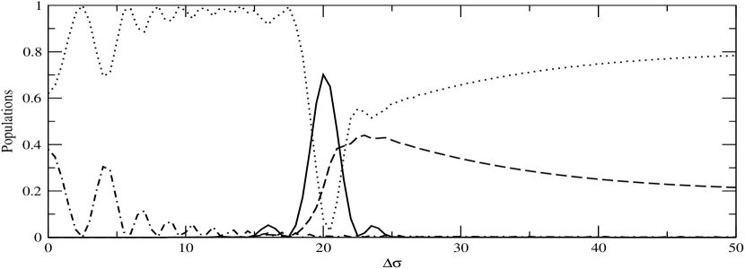
Figure 6: The final populations for the states $|0;e_{1},e_{2}\rangle$ (solid), $|1;g_{1},e_{2}\rangle$ (dot), $|2;g_{1},g_{2}\rangle$ (dot-dashed) and $|1;e_{1},g_{2}\rangle$ (dashed). This latter state was chosen to be the initial state of the system. The parameters are: $\delta=1.0$, $n=0$, $g_{1}\sigma=50$, $\epsilon=1.0$ and $-6\sigma\leq\ t\leq 6\sigma$. The populations were calculated at $t=6\sigma$. Notice the evidence for tri-partite entanglement when $\Delta\sigma\sim 20$.

4 Effects due to cavity losses

The results from the previous sections were derived without taking into account the cavity decoherence due to photon losses. In order to understand the importance of decoherence, we solved the master equation for the density matrix $\rho(t)$ of the entire atom-cavity system,

$$\frac{d\rho}{dt}=-\dot{\imath}\left[H_{I}(t),\rho\right]+\mathcal{L}(\rho).$$ (29)

The term $\mathcal{L}(\rho)$ describes the damping of the field mode with a rate $\gamma$ into an empty thermal reservoir at zero temperature Scully

$$\mathcal{L}(\rho)=-\frac{\gamma}{2}\left(a^{\dagger}a\rho+\rho a^{\dagger}a-2a\rho a^{\dagger}\right).$$ (30)

The main result of the simulations with Eq. (29), is that, as expected, the predictions of the previous sections will hold as long as the cavity losses are substantially suppressed. For example, in figure 7 the fidelity for the maximally entangled state is plotted with respect to $\gamma$. As long as the decay rate $\gamma$ is much smaller than $1/\sigma$, then the fidelity remains large, of the order of unity. For a micromaser cavity with $Q\sim 10^{7}$, a photon lifetime $160\mu s$ and $\sigma\sim 20\mu s$ Brune1996 , the decay rate is approximately $\gamma\sigma=0.125$. For such a cavity the fidelity is just less than $0.9$, figure 7. On the other hand, for a micromaser cavity with $Q\sim 10^{10}$, a photon lifetime is $0.1s$, and the interaction time $\sigma$ of the order of $100\mu s$ Varcoe2004 , the decay rate is approximately $\gamma=10^{-3}/\sigma$. For this decay rate the fidelity is $F\approx 1-10^{-4}$. Both cases are shown in figure 7: $\gamma\sigma=10^{-3}$ marked with an asterisk and $\gamma\sigma=0.125$ with a cross. Thus, the system dynamics can be well described in terms of the ideal model in the absence of decoherence in practical cases, such as the high $Q$ cavity example with $Q\sim 10^{10}$.

5 Conclusion

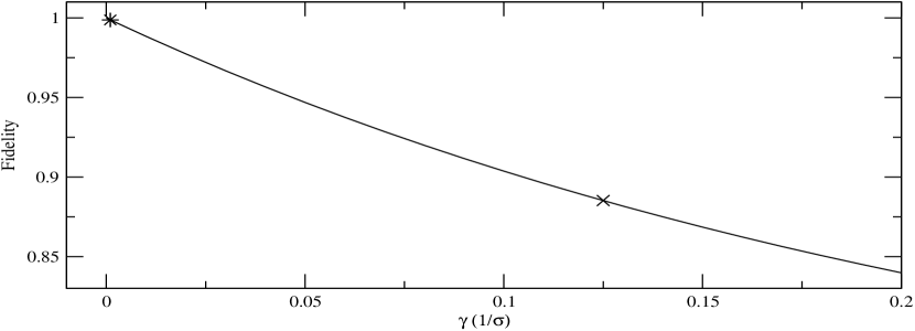
Figure 7: The fidelity for the maximally entangled state $\left|\Psi_{f}(0,2\pi)\right\rangle$ Eq. (20) (solid line) with respect to the decay rate $\gamma$. The curve was found by integrating Eq. (29) for many different decay rates with $\Delta\gamma=0.01/\sigma$. The special points marked $(\ast)$ and $(\times)$ are discussed in detail in the text. The parameters are: $\delta=1.0$, $\epsilon=1.0$, $g_{0}\sigma=18.9286$, $\Delta=0$ and $-12\sigma\leq t\leq 12\sigma$. The fidelity was calculated for $t=12\sigma$. For this choise of coupling the fidelity is equal to one for $\gamma=0$.

In this paper, we examine a system of two atoms interacting with a single mode cavity. Assuming that the atoms enter the cavity at different times, and follow different trajectories inside the cavity, we utilise a cavity-atom interaction with sequential time dependent coupling profiles. We have studied the importance of asymmetries between the atomic coupling profiles. In general the behaviour of the unbalanced system is similar to the ideal case when the coupling profiles are identical in shape. The atom that enters the cavity second is entangled to the cavity mode, whereas the first atom is not. This is due to the existence of an energy crossing in the adiabatic spectrum. Furthermore, the entanglement is defined by the initial state of the second atom, and the degree of entanglement is a function of two mixing angles. Both mixing angles are functions of the coupling strength, the interaction time and the asymmetry factor.

The proposed teleportation protocol remains fairly robust since the system control is a function of only one mixing angle. This is due to the fact that the states involved in the protocol belong to a subspace of the general Hilbert space with a single excitation. Within this subspace, one of the mixing angles is by definition zero. On the other hand, the generation of a maximally entangled state is rather sensitive to variations of the asymmetry factor, with an intense oscillatory fidelity. For an asymmetry factor $\epsilon\approx 0.99$ the fidelity drops to $0.8$, where as for $\epsilon\approx 0.96$ the fidelity is zero.

For off-resonance interactions, the system is characterised by three distinct dynamic regimes. For small detuning, the system qualitatively behaves in a similar way as in the resonant limit. The second atom entangles to the cavity where the entanglement is a function of the detuning and the remaining system parameters. For moderate detunings, both atoms entangle to the cavity this being due to three avoided crossings in the adiabatic spectrum. For a detuning larger than the coupling, the cavity decouples from the system evolution and atoms interact with each other via virtual excitations of the cavity. The system evolves inside a two dimensional phase space, and the fidelity for a maximally entangled state has an extreme behaviour with respect to one of the phase parameters. On the other hand even with a finite detuning the robust state mapping between atoms is valid.

A potential experimental realization of the current model requires a high $Q$ micromaser in order to suppress the cavity losses. A cavity with small quality factor, $Q\sim 10^{7}$ is in practice substantially affected by decoherence effects reducing the fidelity of the proposed applications by a factor greater than $10\%$. On the other hand, for a cavity with $Q$ of the order of $10^{10}$, the decoherence is found to have negligible effects on the system evolution. For example, with such a cavity the fidelity of a maximally entangled state reduces only by $0.2\%$.

- (1) M.A. Nielsen, I.L. Chuang, Quantum computation and quantum information (Cambridge University Press, Cambridge, 2000)
- (2) S.B. Zheng, Phys. Rev. A 71(6), 062335 (2005)
- (3) S.B. Zheng, G.C. Guo, Phys. Rev. Lett. 85(11), 2392 (2000)
- (4) E. Jané, M.B. Plenio, D. Jonathan, Phys. Rev. A 65(5), 050302 (2002)
- (5) L. You, X.X. Yi, X.H. Su, Phys. Rev. A 67(3), 032308 (2003)
- (6) C. Marr, A. Beige, G. Rempe, Phys. Rev. A 68(3), 033817 (2003)
- (7) L. Yong, C. Bruder, C.P. Sun, Phys. Rev. A 75(3), 032302 (2007)
- (8) M.B. Plenio, S.F. Huelga, A. Beige, P.L. Knight, Phys. Rev. A 59(3), 2468 (1999)
- (9) A. Beige, S. Bose, D. Braun, S. Huelga, P. Knight, M. Plenio, V. Vedral, Journal of Modern Optics 47, 2583 (20 November 2000)
- (10) A. Beige, D. Braun, B. Tregenna, P.L. Knight, Phys. Rev. Lett. 85(8), 1762 (2000)
- (11) A.S. Sørensen, K. Mølmer, Phys. Rev. Lett. 90(12), 127903 (2003)
- (12) T.W. Chen, C.K. Law, P.T. Leung, Phys. Rev. A 68(5), 052312 (2003)
- (13) L.M. Duan, H.J. Kimble, Phys. Rev. Lett. 90(25), 253601 (2003)
- (14) C. Lazarou, B. Garraway, Adiabatic entanglement in two-atom cavity QED. Submitted
- (15) A. Messiah, Quantum Mechanics (Dover Publications, New York, 1999)
- (16) S. Mahmood, M.S. Zubairy, Phys. Rev. A 35(1), 425 (1987)
- (17) K. Bergmann, H. Theuer, B.W. Shore, Rev. Mod. Phys. 70(3), 1003 (1998)
- (18) K. Bergmann, B.W. Shore, in Molecular Dynamics and Spectroscopy by Stimulated Emission Pumping, edited by H.L. Dai, R.W. Field (World Scientific, Singapore, 1995), chap. 9, pp. 315–73
- (19) See for example M.O. Scully, M.S. Zubairy, Quantum Optics (Cambridge University Press, Cambridge, 2002)
- (20) M. Brune, E. Hagley, J. Dreyer, X. Maître, A. Maali, C. Wunderlich, J.M. Raimond, S. Haroche, Phys. Rev. Lett. 77(24), 4887 (1996)
- (21) B.T.H Varcoe, H. Walther, New Journal of Physics 6, 97 (2004)