Effect of detector dead-times on the security evaluation of differential-phase-shift quantum key distribution against sequential attacks

Abstract

We investigate limitations imposed by detector dead-times on the performance of sequential attacks against a differential-phase-shift (DPS) quantum key distribution (QKD) protocol with weak coherent pulses. In particular, we analyze sequential attacks based on unambiguous state discrimination of the signal states emitted by the source and we obtain ultimate upper bounds on the maximal distance achievable by a DPS QKD scheme both in the so-called trusted and untrusted device scenarios, respectively.

I INTRODUCTION

Quantum key distribution (QKD) gisin_rev_mod is a technique that allows two parties (usually called Alice and Bob) to generate a secret key despite the computational and technological power of an eavesdropper (Eve) who interferes with the signals. Together with the Vernam cipher vernam , QKD can be used for unconditionally secure data transmission.

The first complete QKD scheme was introduced by Bennett and Brassard in 1984 (BB84 for short) BB84 . An unconditional security proof for the whole protocol has been given in Ref. Mayers98 . After the first demonstration of the feasibility of this scheme Bennett92 , several long-distance implementations of QKD have been realized in the last years (see, for instance, Ref. Marand95 and references therein). However, these practical approaches differ in many important aspects from the original theoretical proposal, since it demands technologies that are beyond our present experimental capability. Especially, the signals emitted by the source, instead of being single-photons, are usually weak coherent pulses (WCP) with typical average photon numbers of $0.1$ or higher. This fact, together with the considerable attenuation introduced by quantum the channel and the noise introduced by the detectors, jeopardize the security of the protocol and lead to limitations of rate and distance that can be covered by these techniques Huttner95 ; Norbert00 . A positive security proof against all individual attacks, even with practical signals, has first been given in Ref. Norbert_individual , while a complete proof of the unconditional security of this scheme in a realistic setting has been provided in Refs. inamori ; inamori2 . This means that, despite practical restrictions, with the support of the classical information techniques (error correction and privacy amplification) used in the key distillation phase, it is still possible to obtain a secure secret key.

The main security threat of QKD protocols based on WCP arises from the fact that some signals contain more than one photon prepared in the same polarization state. Now, Eve can perform, for instance, the so-called Photon Number Splitting (PNS) attack on the multi-photon pulses Huttner95 . This attack provides Eve with full information about the part of the key generated from the multi-photon signals, without causing any disturbance in the signal polarization. As a result, it turns out that the BB84 protocol with WCP can give a key generation rate of order $O(\eta^{2})$, where $\eta$ denotes the transmission efficiency of the quantum channel inamori ; inamori2 .

To obtain higher secure key rates over longer distances, different QKD schemes, that are robust against the PNS attack, have been proposed in recent years. One of these schemes is the so-called decoy-states decoy_t ; decoy_e , where Alice varies at random the mean photon number of the signal states sent to Bob by using different intensity settings. This technique delivers a key generation rate of order $O(\eta)$ decoy_t ; decoy_e . Another possibility is based on the transmission of two non-orthogonal coherent states together with a strong reference pulse ben92 . This scheme has been analyzed in detail in Ref. koashi04 , where it was confirmed that also in this scenario the secure key rate is of order $O(\eta)$. Finally, another possible approach is to use a differential-phase-shift (DPS) QKD protocol dpsqkd ; dpsqkd2 ; dpsqkd_exp1 ; dpsqkd_exp2 ; dpsqkd_exp2b ; dpsqkd_exp3 . In this scheme Alice sends to Bob a train of WCP whose phases are randomly modulated by $0$ or $\pi$. On the receiving side, Bob measures out each incoming signal by means of an interferometer whose path-length difference is set equal to the time difference between two consecutive pulses. In this last case, however, a secure key rate of order $O(\eta)$ has only been proven so far against a special type of individual attacks where Eve acts and measures photons individually, rather than signals dpsqkd2 , and also against a particular class of collective attacks where Eve attaches ancillary systems to each pulse or to each pair of successive pulses cyril_new . While a complete security proof of DPS QKD against the most general attack is still missing, recently it has been shown that sequential attacks already impose strong restrictions on the performance of this QKD scheme with WCP dpsqkd2 ; curty_dps ; tsurumaru_dps . For instance, it was proven in Refs. curty_dps ; tsurumaru_dps that the DPS QKD experiments reported in Refs. dpsqkd_exp1 ; dpsqkd_exp2 are insecure against this type of attacks. Basically, a sequential attack consists of Eve measuring out every signal state emitted by Alice and, afterwards, she prepares new signal states, depending on the results obtained, that are given to Bob. Whenever Eve obtains a predetermined number of consecutive successful measurement outcomes, then she prepares a train of non-vacuum signal states that is forwarded to Bob. Otherwise, Eve sends, for instance, vacuum signals to Bob to avoid errors. Sequential attacks constitute a special type of intercept-resend attacks jahma01 ; Felix01 ; curty05 and, therefore, they provide ultimate upper bounds on the performance of QKD schemes Curty04 .

In discussions within the scientific community one often hears, however, that the security analysis presented in Refs. curty_dps ; tsurumaru_dps might have overestimated the strength that sequential attacks have against a DPS QKD protocol. This conjecture is justified because the sequential attacks studied so far in the literature have not considered the effect of Bob’s detectors dead-time. As a result, the probability that each non-vacuum signal state, within a train of them, sent by Eve contributes to the sifted key does not depend on whether the previous signal states in the train already produced a click on Bob’s detection apparatus or not. This suggests that such analysis might overestimate the number of Bob’s detected events that originates from the non-vacuum signal states sent by Eve and, therefore, it might deliver shorter secure distances.

The aim of this paper is to investigate limitations imposed by Bob’s detectors dead-time on the performance of sequential attacks against a DPS QKD protocol note1 . For that, we shall analyze sequential attacks based on unambiguous state discrimination (USD) of the signal states emitted by Alice curty_dps ; tsurumaru_dps ; usd ; chef ; jahma01 . When Eve identifies unambiguously a signal state, then she considers this result as successful. Otherwise, she considers it a failure. We shall consider two possible scenarios for our analysis. The first one, so-called untrusted device scenario, arises from a conservative definition of security, i.e., we shall assume that Eve can control some imperfections in Alice and Bob’s devices (e.g., the detection efficiency, the dark count probability, and the dead-time of Bob’s detectors), together with the losses in the quantum channel, and she exploits them to obtain maximal information about the shared key. In the second scenario, so-called trusted device scenario, we shall consider that Eve cannot modify the actual detection devices employed by Alice and Bob. That is, the legitimate users have complete knowledge about their detectors, which are fixed by the actual experiment. The main motivation to study this scenario is that, from a practical point of view, it constitutes a reasonable description of a realistic situation, where Alice and Bob can limit Eve’s influence on their apparatus by some counterattack techniques Note6 .

A different QKD scheme, but also related to a DPS QKD protocol, has been proposed recently in Ref. stucki_new . (See also Ref. gisin_new .) However, since the abstract signal structure of this protocol is different from the one of a DPS QKD scheme, the analysis contained in this paper does not apply to that scenario. Sequential attacks against the QKD protocol introduced in Ref. stucki_new have been investigated in Ref. bran_new , while its security against a particular class of collective attacks has been studied in Ref. cyril_new .

The paper is organized as follows. In Sec. II we describe in more detail a DPS QKD protocol. Then, in Sec. III, we present sequential attacks against this QKD scheme. Section IV includes the analysis for the untrusted device scenario. Here we obtain an upper bound on the maximal distance achievable by a DPS QKD protocol as a function of the error rate in the sifted key, the mean photon-number of Alice’s signal states and the dead-time of Bob’s detectors. Similar results are derived in Sec. V, now for the trusted device scenario. Finally, Sec. VI concludes the paper with a summary. The manuscript includes as well several appendices with additional calculations.

II DIFFERENTIAL-PHASE-SHIFT (DPS) QKD

The setup is illustrated in Fig. 1 dpsqkd ; dpsqkd2 ; dpsqkd_exp1 ; dpsqkd_exp2 ; dpsqkd_exp2b ; dpsqkd_exp3 .

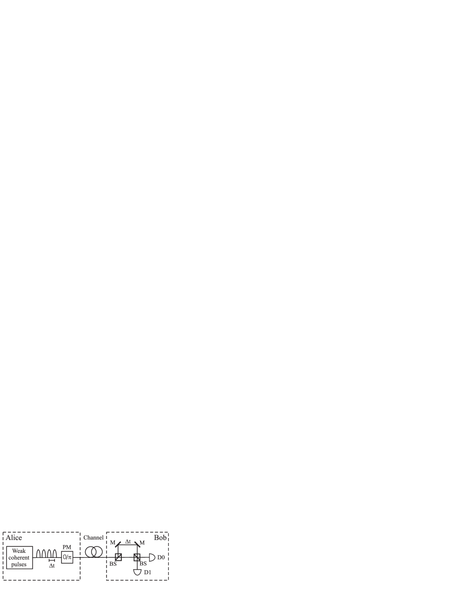
Figure 1: Basic setup of a DPS QKD scheme. PM denotes a phase modulator, BS, a $50:50$ beam splitter, M, a mirror, D0 and D1 are two photon detectors and $\Delta{}t$ represents the time difference between two consecutive pulses.

Alice prepares first a train of coherent states $|\alpha\rangle$ and, afterwards, she modulates, at random and independently every time, the phase of each pulse to be $0$ or $\pi$. As a result, she produces a random train of signal states $|\alpha\rangle$ or $|-\alpha\rangle$ that are sent to Bob through the quantum channel. On the receiving side, Bob uses a $50:50$ beam splitter to divide the incoming pulses into two possible paths and then he recombines then again using another $50:50$ beam splitter. The time delay introduced by Bob’s interferometer is set equal to the time difference $\Delta{}t$ between two pulses. Whenever the relative phase between two consecutive signals is $0$ ($\pm\pi$) only the photon detector $D0$ ($D1$) may produce a “click” (at least one photon is detected). For each detected event, Bob records the time slot where he obtained a click and the actual detector that fired.

Once the quantum communication phase is completed, Bob uses a classical authenticated channel to announce the time slots where he obtained a click, but he does not reveal which detector fired each time. From this information provided by Bob, together with the knowledge of the phase value used to modulate each pulse, Alice might infer which photon detector had clicked at Bob’s side each given time. Then, Alice and Bob can agree, for instance, to select a bit value “0” whenever the photon detector $D0$ fired, and a bit value “1” if the detector $D1$ clicked. In an ideal scenario, Alice and Bob end up with an identical string of bits representing the sifted key. Due to the noise introduced by the quantum channel, together with possible imperfections of Alice and Bob’s devices, however, the sifted key typically contains some errors. Then, Alice and Bob perform error-correction to reconcile the data and privacy amplification to decouple the data from Eve. (See, for instance, Ref. gisin_rev_mod .)

III Sequential attacks against DPS QKD

A sequential attack can be seen as a special type of intercept-resend attack dpsqkd2 ; curty_dps ; tsurumaru_dps . First, Eve measures out every coherent state emitted by Alice with a detection apparatus located very close to the sender. Afterwards, she transmits each measurement result through a lossless classical channel to a source close to Bob. Whenever Eve considers a sequence of measurement outcomes successful, this source prepares a new train of signal states that is forwarded to Bob. Otherwise, Eve typically sends vacuum signals to Bob to avoid errors. Whether a sequence of measurement results is considered to be successful or not, and which type of non-vacuum signal states Eve sends to Bob, depends on Eve’s particular eavesdropping strategy and on her measurement device. Sequential attacks transform the original quantum channel between Alice and Bob into an entanglement breaking channel Horodecki03 and, therefore, they do not allow the distribution of quantum correlations needed to establish a secret key Curty04 .

Let us begin by introducing Eve’s measurement apparatus. As mentioned previously, we shall consider that Eve realizes USD usd ; chef of each signal state sent by Alice. That is, whenever she obtains a conclusive result then it is guaranteed that the result is always correct. In order to do that, we will assume that Eve has always access to a local oscillator that is phase-locked to the coherent light source employed by Alice Note2 . Whenever Eve identifies unambiguously a predetermined number of consecutive signal states, i.e., she determines without error whether each signal state is $|\alpha\rangle$ or $|-\alpha\rangle$, she considers this sequence of measurement outcomes successful. Otherwise she considers it a failure Note3 . We define the integer parameter $M_{min}$ as the minimum number of consecutive USD successful results that Eve needs to obtain in order to consider the sequence of measurement outcomes successful. More precisely, if $k\geq{}0$ denotes the total number of consecutive USD successful outcomes obtained by Eve before she obtains an inconclusive result, then, whenever $k>M_{min}$, Eve prepares a new train of signal states, that we shall denote as $\rho_{e}^{k}$, together with some vacuum states for the inconclusive result, and she sends these signals to Bob. The precise definition of the quantum state $\rho_{e}^{k}$ will be introduced later on, since it will depend on whether we consider the untrusted or the trusted device scenario, respectively. The reason to append some vacuum states to each train of signal states $\rho_{e}^{k}$ is also closely related to the eavesdropping strategy of these two possible cases. The main idea behind this procedure is to guarantee that whenever Bob obtains a click on his detection apparatus then he cannot obtain any other click afterwards during a period of time at least equal to the dead-time of his detectors. That is, these vacuum states sent by Eve will allow her to reproduce the dead-time of Bob’s detectors, whose influence on the security evaluation of a DPS QKD protocol is the main focus of this paper. For simplicity, let us assume for the moment that Eve sends to Bob $1+d$ vacuum states together with each train of signal states $\rho_{e}^{k}$ in order to achieve this goal, while the precise value of the parameter $d$ will be given for the untrusted (trusted) device scenario in Sec. IV (Sec. V). On the other hand, if $k<M_{min}$ Eve sends to Bob $k+1$ vacuum states, where the last vacuum state corresponds to Eve’s inconclusive result. The case $k=M_{min}$ deserves special attention. We shall consider that in this situation Eve employs a probabilistic strategy that combines the two previous ones. In particular, we assume that Eve sends to Bob the signal state $\rho_{e}^{M_{min}}$, together with $1+d$ vacuum states, with probability $q$ and, with probability $1-q$, she sends to Bob $M_{min}+1$ vacuum states. That is, the parameter $q$ allows Eve to smoothly fit her eavesdropping strategy to the observed data curty_dps . Moreover, in order to simplify our calculations, we define the integer parameter $M_{max}>M_{min}$ as the maximum number of consecutive USD successful results that Eve can obtain in order to send to Bob a train of signal states. That is, whenever Eve obtains $M_{max}$ consecutive USD successful outcomes then she discards the next measurement outcome and directly sends to Bob the quantum state $\rho_{e}^{M_{max}}$ together with $1+d$ vacuum states for the discarded measurement result.

Let $p$ denote the probability that Eve obtains an USD successful result per signal state sent by Alice. It has the following form usd

$$p=1-|\mbox{$\langle\alpha|$}-\alpha\rangle|=1-\exp{(-2\mu_{\alpha})},$$ (1)

where $\mu_{\alpha}$ represents the mean photon-number of Alice’s signal states, i.e., $\mu_{\alpha}=|\alpha|^{2}$.

We shall denote with $p_{s}(k)$ the probability that Eve sends to Bob a train of signal states $\rho_{e}^{k}$, together with $1+d$ vacuum states. This probability can be written as

$$p_{s}(k)=\left\{\begin{array}[]{ll}qp^{M_{min}}(1-p)&\textrm{if $k=M_{min}$}\\ p^{k}(1-p)&\textrm{if $M_{min}<k<M_{max}$}\\ p^{M_{max}}&\textrm{if $k=M_{max}$}\\ 0&\textrm{otherwise,}\end{array}\right.$$ (2)

with $p$ given by Eq. (1). Similarly, we shall denote with $p_{v}(k)$ the probability that Eve sends to Bob $k+1$ vacuum states. This probability is given by

$$p_{v}(k)=\left\{\begin{array}[]{ll}p^{k}(1-p)&\textrm{if $0\leq{}k<M_{min}$}\\ (1-q)p^{M_{min}}(1-p)&\textrm{if $k=M_{min}$}\\ 0&\textrm{otherwise.}\end{array}\right.$$ (3)

We illustrate all these possible cases in Fig. 2, where we also include the different a priori probabilities to be in each of these scenarios.

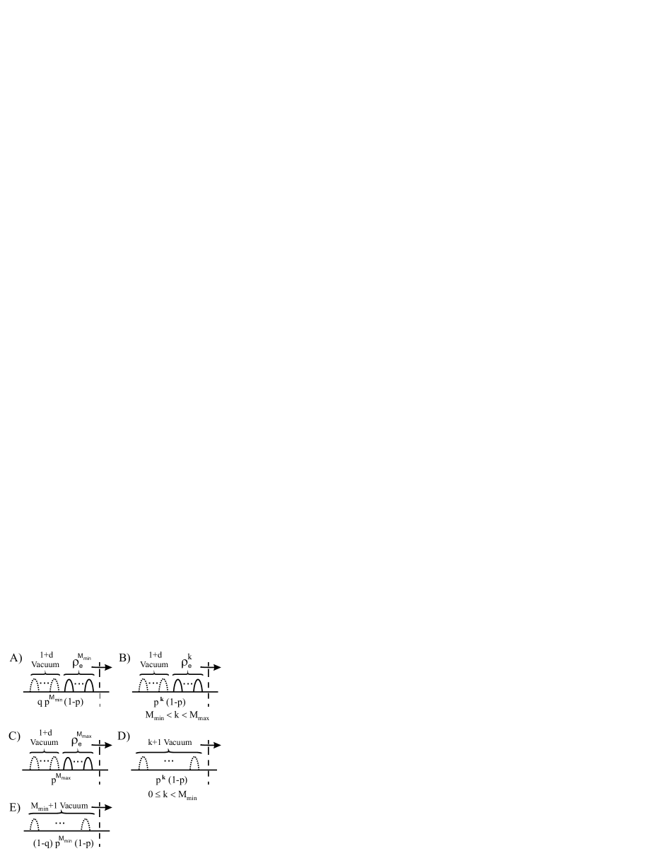
Figure 2: Possible signal states that Eve sends to Bob together with their a priori probabilities. The arrow indicates the transmission direction.

Next we analyze in detail the influence that Bob’s detectors dead-time has on the performance of the sequential attack introduced above. The goal is to find an expression for the gain, i.e., the probability that Bob obtains a click per signal state sent by Alice, together with the quantum bit error rate (QBER) introduced by Eve, in both the untrusted and the trusted device scenarios, respectively.

IV Untrusted device scenario

Here we shall consider that Eve can always control some imperfections in Alice and Bob’s devices together with the quantum channel. Especially, we shall assume that Eve can always replace Bob’s imperfect detection apparatus by an ideal one in order to exploit its detection efficiency, together with the dark count probability and the dead-time of his detectors, to obtain maximal information about the shared key. Of course, to guarantee that Eve’s presence remains unnoticeable to the legitimate users, Eve needs to send Bob signal states that can reproduce the statistics that Alice and Bob expect after their measurements. For this, we shall consider the standard version of a DPS QKD protocol, where Alice and Bob only monitor the raw bit rate (before the key distillation phase) together with the time instances in which Bob obtains a click.

The main limitation on the type of signal states that Eve can send to Bob in this scenario arises from the dead-time of Bob’s detectors. In order to simplify our analysis we shall assume that both detectors $D0$ and $D1$ in Fig. 1 are indistinguishable, i.e., their dark count rate, quantum efficiency and dead-time, are equal. Moreover, we shall consider a conservative scenario where every time that one of these detectors clicks, then both detectors do not respond to any other incident photon during a period of time equal to the dead-time, i.e., we shall assume that after a click both detectors suffer simultaneously from a dead time. This is a key assumption underlying the whole analysis presented in this paper. In the experimental setup employed in Refs. dpsqkd_exp1 ; dpsqkd_exp2 ; dpsqkd_exp2b ; dpsqkd_exp3 both detectors $D0$ and $D1$ are connected to the same Time Interval Analyser (TIA) that also has a dead-time which is typically much higher than the dead-time of the detectors. Whenever one of these detectors clicks then the TIA does not respond to any other click event during a period of time equal to its dead-time. In this situation, however, if $D0$ and $D1$ do not suffer simultaneously from a dead-time, then the effect of the TIA can be understood as just blocking some of the output signals coming from the two detectors. As a result, the raw key obtained by Alice and Bob could contain correlations between different bits which might be known to some extend to Eve. For instance, if one detector clicks, and the clock frequency of the system is high enough, then, because of its dead-time, it is more probable that the next click comes from the other detector. This last scenario is beyond the scope of this paper and the analysis will be presented somewhere else.

In the sequential attack introduced in Sec. III, Eve sends to Bob only two possible classes of signal states: a state $\rho_{e}^{k}$ followed by $1+d$ vacuum states, or a train of $k+1$ vacuum signals. This means, in particular, that Bob can only obtain clicks in his detection apparatus when he receives a signal state $\rho_{e}^{k}$. To be able to mimic the dead-time of Bob’s detectors, therefore, Eve needs to select each state $\rho_{e}^{k}$ such that it can produce only one click on Bob’s side within a dead-time period. For that, Eve chooses $\rho_{e}^{k}$ containing only one photon distributed among $k$ temporal modes. These modes correspond to $k$ consecutive pulses sent by Alice, i.e., the time difference between two consecutive temporal modes in $\rho_{e}^{k}$ is set equal to the time difference $\Delta{}t$ between two consecutive pulses sent by Alice. More precisely, we shall consider that $\rho_{e}^{k}$ denotes a pure state $|\psi_{e}^{k}\rangle$ (i.e., $\rho_{e}^{k}=\mbox{$|\psi_{e}^{k}\rangle$}\mbox{$\langle\psi_{e}^{k}|$}$) given by

$$\mbox{$|\psi_{e}^{k}\rangle$}=\sum_{n=1}^{k}A_{n}^{(k)}\exp{(i\theta_{n})}\hat{a}_{n}^{\dagger}\mbox{$|0\rangle$},$$ (4)

with $A_{n}^{(k)}\in\mathbb{C}$ and where the normalization condition $\sum_{n=1}^{k}|{}A_{n}^{(k)}|{}^{2}=1$ is always satisfied. The angles $\theta_{n}$ fulfill $\theta_{n}=0$ if the signal state identified by Eve’s USD measurement at the time instance $n$ is $|\alpha\rangle$ and $\theta_{n}=\pi$ if the signal state identified by Eve is $|-\alpha\rangle$, the operator $\hat{a}_{n}^{\dagger}$ represents a creation operator for one photon in temporal mode $n$, and the state $|0\rangle$ refers to the vacuum state. Eq. (4) considers the possibility of using different amplitudes $A_{n}^{(k)}$ for the resent signals, following the spirit of Ref. tsurumaru_dps . The superscript $k$ labeling the coefficients $A_{n}^{(k)}$ emphasizes the fact that the value of these coefficients may depend on the number of temporal modes $k$ contained in $|\psi_{e}^{k}\rangle$. Moreover, from now on we will use the convention that the first temporal mode of $|\psi_{e}^{k}\rangle$ that arrives at Bob’s detection device is mode $n=k$, while the last one is mode $n=1$. This labeling convention is illustrated in Fig. 3.

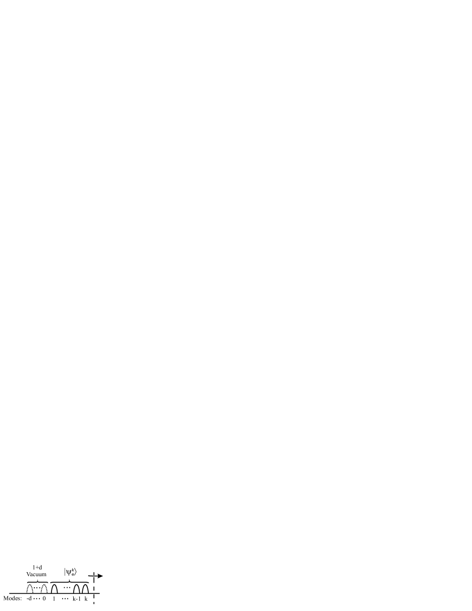
Figure 3: Labeling convention for the $k$ temporal modes of the signal state $|\psi_{k}\rangle$ given by Eq. (4) followed by $1+d$ vacuum states. The arrow indicates the transmission direction.

Let us now determine the minimum number, $1+d$, of vacuum states that Eve needs to send to Bob after each signal state $|\psi_{e}^{k}\rangle$. From the previous paragraph we learn that whenever Bob receives a state $|\psi_{e}^{k}\rangle$ satisfying Eq. (4) then he obtains one single click in his detection device. This click can occur, however, in any temporal mode $n$, with $n\in[0,k]$ Note5 . The minimum value of the parameter $d$ can be calculated from the case where Bob obtains a click in the last possible temporal mode, i.e., $n=0$ (see Fig. 3). Let us assume that such a click occurs, and let $t_{d}$ and $f_{c}$ denote, respectively, the dead-time of Bob’s detectors and the clock frequency of the system. To guarantee that Bob cannot obtain any other click from a following signal state until $t_{d}$ finishes we find that $d$ has to fulfill $d\geq\lceil{}t_{d}f_{c}\rceil$. That is, the parameter $d$ has to be larger than or equal to the number of signal states sent by Alice within a period of time equal to the dead-time. From now on we shall consider that Eve selects $d$ such that

$$d=\lceil{}t_{d}f_{c}\rceil.$$ (5)

Next, we obtain an expression for the gain and for the QBER introduced by Eve in this scenario.

IV.1 Gain

The gain, that we shall denote as $G$, of a sequential attack is defined as the probability that Bob obtains a click per signal state sent by Alice. It can be expressed as $G=N_{clicks}/N$, where $N_{clicks}$ represents the average total number of clicks obtained by Bob, and $N$ is the total number of signal states sent by Alice. The parameter $N_{clicks}$ can be expressed as $N_{clicks}=(N/N^{e})N_{clicks}^{e}$, with $N^{e}$ denoting the average total number of pulses of signal states sent by Eve (see Fig. 2), and where $N_{clicks}^{e}$ represents the average total number of clicks obtained by Bob when Eve sends to him precisely these signal states. With this notation, the gain of a sequential attack can be written as

$$G=\frac{N_{clicks}^{e}}{N^{e}}.$$ (6)

Next, we obtain an expression for $N_{clicks}^{e}$ and $N^{e}$. Let us begin with $N_{clicks}^{e}$. Whenever Eve sends to Bob a signal state $|\psi_{e}^{k}\rangle$ followed by $1+d$ vacuum states (Cases A, B, and C in Fig. 2) Bob always obtains one click in his detection apparatus. On the other hand, if Eve sends to Bob only vacuum states (Cases D and E in Fig. 2) Bob never obtains a click. This means, in particular, that $N_{clicks}^{e}$ can be expressed as

$$N_{clicks}^{e}=\sum_{k=M_{min}}^{M_{max}}p_{s}(k),$$ (7)

with $p_{s}(k)$ given by Eq. (2). This expression can be further simplified as

$$N_{clicks}^{e}=\big{[}q+(1-q)p\big{]}p^{M_{min}}.$$ (8)

The analysis to obtain $N^{e}$ is similar. A signal state $|\psi_{e}^{k}\rangle$ followed by $1+d$ vacuum states can be seen as containing $k+1+d$ pulses. On the other hand, the number of vacuum pulses alone that Eve sends to Bob can vary from $1$ to $M_{min}+1$ (see Fig. 2). Adding all these terms together, and taking into account their a priori probabilities, we obtain that $N^{e}$ can be written as

$$N^{e}=\sum_{k=0}^{M_{max}}p_{v}(k)(k+1)+p_{s}(k)(k+1+d),$$ (9)

with $p_{v}(k)$ given by Eq. (3). This expression can be simplified as

$$N^{e}=\frac{d\big{[}q+(1-2q)p-(1-q)p^{2}\big{]}p^{M_{min}}-p^{M_{max}+1}+1}{1-p}$$ (10)

The gain $G$ can be related with a transmission distance $l$ for a given QKD scheme, i.e., a distance which provides an expected click rate at Bob’s side given by $G$. This last condition can be written as

$$G=1-\exp{(-\mu_{\alpha}\eta_{det}\eta_{t})},$$ (11)

where $\eta_{det}$ represents the detection efficiency of the detectors employed by Bob, and $\eta_{t}$ denotes the transmittivity of the quantum channel. In the case of a DPS QKD scheme, the value of $\eta_{t}$ can be derived from the loss coefficient $\gamma$ of the optical fiber measured in dB/km, the transmission distance $l$ measured in km, and the loss in Bob’s interferometer $L$ measured in dB as

$$\eta_{t}=10^{-\frac{\gamma{}l+L}{10}}.$$ (12)

From Eq. (11) and Eq. (12), we find that the transmission distance $l$ that provides a gain $G$ is given by

$$l=-\frac{1}{\gamma}\bigg{[}L+10\log_{10}\bigg{(}\frac{-\ln{(1-G)}}{\mu_{\alpha}\eta_{det}}\bigg{)}\bigg{]}.$$ (13)

IV.2 Quantum bit error rate

The QBER, that we shall denote as $Q$, is defined as $Q=N_{errors}/N_{clicks}$, where $N_{errors}$ represents the average total number of errors obtained by Bob, and $N_{clicks}$ is again the average total number of clicks at Bob’s side. The parameter $N_{errors}$ can be expressed as $N_{errors}=(N/N^{e})N_{errors}^{e}$, with $N_{errors}^{e}$ denoting the average total number of errors obtained by Bob when Eve sends him the different signal states considered in her strategy (see Fig. 2). With this notation, and using again the fact that $N_{clicks}=(N/N^{e})N_{clicks}^{e}$, we obtain that the QBER of a sequential attack can be expressed as

$$Q=\frac{N_{errors}^{e}}{N_{clicks}^{e}}.$$ (14)

The parameter $N_{clicks}^{e}$ was calculated in the previous section and it is given by Eq. (8). Let us now obtain an expression for $N_{errors}^{e}$. We shall distinguish the same cases like in the previous section, depending on the type of signal states that Eve sends to Bob. Whenever Eve sends to Bob a signal state $|\psi_{e}^{k}\rangle$ followed by $1+d$ vacuum states (Cases A, B, and C in Fig. 2) then we shall denote the average total number of errors in this scenario as $e(k)$. On the other hand, if Eve sends to Bob only vacuum states (Cases D and E in Fig. 2) Bob never obtains an error. This means, in particular, that $N_{errors}^{e}$ can be expressed as

$$N_{errors}^{e}=\sum_{k=M_{min}}^{M_{max}}p_{s}(k)e(k).$$ (15)

The parameters $e(k)$, with $M_{min}\leq{}k\leq{}M_{max}$, can be obtained from the signal states $|\psi_{e}^{k}\rangle$, together with the detection device used by Bob. They are calculated in Appendix A and are given by

$$e(k)=\frac{1}{4}\Bigg{[}|{}A_{1}^{(k)}|{}^{2}+\sum_{n=1}^{k-1}|{}A_{n+1}^{(k)}-A_{n}^{(k)}|{}^{2}+|{}A_{k}^{(k)}|{}^{2}\Bigg{]}.$$ (16)

IV.3 Evaluation

We have seen above that a sequential attack can be parametrized by the minimum number $M_{min}$ of consecutive USD successful results that Eve needs to obtain in order to consider the sequence of measurement outcomes successful, the maximum number $M_{max}$ of consecutive successful results that Eve can obtain in order to send to Bob a train of signal states, the value of the probability $q$, i.e., the probability that Eve actually decides to send to Bob the signal state $|\psi_{e}^{M_{min}}\rangle$ followed by $1+d$ vacuum states instead of $M_{min}+1$ vacuum states, and the state coefficients $A_{n}^{(k)}\in\mathbb{C}$ that characterize the signal states $|\psi_{e}^{k}\rangle$, with $M_{min}\leq{}k\leq{}M_{max}$.

Figures 4, 5, 6 and 7 show a graphical representation of the Gain versus the QBER in this sequential attack for different values of the mean photon-number $\mu_{\alpha}$ of Alice’s signal states, the parameter $d$, and the state coefficients $A_{n}^{(k)}$. It states that no key distillation protocol can provide a secret key from the correlations established by the users above the curves, i.e., the secret key rate in that region is zero. In these examples we consider three possible distributions for $A_{n}^{(k)}$: the flat distribution, the binomial distribution, and we also calculate the optimal distribution, i.e., the one which provides the lowest QBER for a given value of the Gain. The corresponding state coefficients for these distributions are given by

Figure 4: Gain ($G$) versus QBER in a sequential attack for three different distributions of the state coefficients $A_{n}^{(k)}$: flat (solid), binomial (dashed), and the optimal distribution (dotted). The mean photon number of Alice’s signal states is $\mu_{\alpha}=0.2$, and the parameter $d=500$. The triangles represent experimental data from Ref. dpsqkd_exp3 .

Figure 5: Gain ($G$) versus QBER in a sequential attack for three different distributions of the state coefficients $A_{n}^{(k)}$: flat (solid), binomial (dashed), and the optimal distribution (dotted). The mean photon number of Alice’s signal states is $\mu_{\alpha}=0.17$, and the parameter $d=50$. The triangles represent experimental data from Ref. dpsqkd_exp1 . (See also Ref. dpsqkd_exp2b .)

Figure 6: Gain ($G$) versus QBER in a sequential attack for three different distributions of the state coefficients $A_{n}^{(k)}$: flat (solid), binomial (dashed), and the optimal distribution (dotted). The mean photon number of Alice’s signal states is $\mu_{\alpha}=0.16$, and the parameter $d=50$. The triangle represents experimental data from Ref. dpsqkd_exp1 . (See also Ref. dpsqkd_exp2b .)

Figure 7: Gain ($G$) versus QBER in a sequential attack for three different distributions of the state coefficients $A_{n}^{(k)}$: flat (solid), binomial (dashed), and the optimal distribution (dotted). The mean photon number of Alice’s signal states is $\mu_{\alpha}=0.2$, and the parameter $d=50$. The triangles represent experimental data from Ref. dpsqkd_exp2 . (See also Ref. dpsqkd_exp2b .)

Flat: $$A^{(k)}_{n}=\frac{1}{\sqrt{k}},\;\text{for all }n\in[1,k],$$

Binomial: $$A^{(k)}_{n}=\left(\frac{1}{\sqrt{2}}\right)^{k-1}\sqrt{\left(\begin{array}[]{c}k-1\\ n-1\end{array}\right)},$$ (19)

while the method to obtain the optimal distribution is described in Appendix B. Figures 4, 5, 6 and 7 assume as well that $M_{max}$ is fixed and given by $M_{max}=25$, and we vary the parameters $M_{min}<M_{max}$ and $q\in[0,1]$. They also include experimental data from Refs. dpsqkd_exp1 ; dpsqkd_exp2 ; dpsqkd_exp2b ; dpsqkd_exp3 . For instance, in the experiment reported in Ref. dpsqkd_exp3 the dead-time of Bob’s detectors is $t_{d}=50$ ns and the clock frequency of the system is $f_{c}=10$ GHz. From Eq. (5) we obtain, therefore, that $d=500$. (See Fig. 4.) Similarly, in the experiments realized in Refs. dpsqkd_exp1 ; dpsqkd_exp2 ; dpsqkd_exp2b we have that $t_{d}=50$ ns and $f_{c}=1$ GHz. This means, in particular, that in all these cases $d=50$. (See Figs. 5, 6 and 7.) According to our results it seems that all the long-distance implementations of DPS QKD reported in Refs. dpsqkd_exp1 ; dpsqkd_exp2 ; dpsqkd_exp2b ; dpsqkd_exp3 would be insecure against a sequential attack in the untrusted device scenario. That is, there exists no improved classical communication protocol or improved security analysis which might allow the data of Refs. dpsqkd_exp1 ; dpsqkd_exp2 ; dpsqkd_exp2b ; dpsqkd_exp3 to be turned into secret key.

V Trusted device scenario

In this section we impose constraints on Eve’s capabilities, and we are interested in the effect that these constraints have on her eavesdropping strategy. In particular, we study the situation where Eve is not able to manipulate Alice and Bob’s devices at all, but she is limited to act exclusively on the quantum channel (See, e.g., Refs. jahma01 ; curty_pns ). That is, we shall consider that the detection efficiency, the dark count probability, and the dead-time of Bob’s detectors are now fixed by the actual experiment, and Eve cannot influence them to obtain extra information about the shared key. The main motivation to analyze this scenario is that, from a practical point of view, it constitutes a reasonable description of a realistic situation, where Alice and Bob could in principle limit Eve’s influence on their apparatus by some counterattack techniques Note6 . Moreover, this could only enhance Alice and Bob’s ability to distill a secret key.

The detection efficiency $\eta_{det}$ of Bob’s detectors typically satisfies $\eta_{det}<1$. Therefore, in this scenario, Eve might be interested in sending Bob multi-photon signals, instead of single-photon states like in Sec. IV, in order to increase the gain. Moreover, as mentioned above, we assume now that the dead-time of Bob’s detectors is already present in $D0$ and $D1$ and Eve does not need to select her signal states such that they can reproduce it. These two facts motivate the following definition for the signal states $\rho_{e}^{k}$ in this case. In particular, we shall consider that $\rho_{e}^{k}$ consists of a classical mixture of pure states, that we shall denote as $|\psi_{k}^{m}\rangle$, containing $m\geq{}1$ photons that are distributed among $k$ temporal modes, i.e.,

$$\rho_{e}^{k}=\sum_{m=1}^{\infty}p_{m}\mbox{$|\psi_{k}^{m}\rangle$}\mbox{$\langle\psi_{k}^{m}|$},$$ (20)

with the photon-number probabilities $p_{m}$ satisfying $\sum_{m=1}^{\infty}p_{m}=1$ Note7 . The states $|\psi_{k}^{m}\rangle$ are defined as

$$\mbox{$|\psi_{k}^{m}\rangle$}=\frac{\big{(}\hat{\psi}_{k,m}^{{\dagger}}\big{)}^{m}}{\sqrt{m!}}\mbox{$|0\rangle$},$$ (21)

with $|0\rangle$ representing the vacuum state, and where the operators $\hat{\psi}_{k,m}^{{\dagger}}$ are given by

$$\hat{\psi}_{k,m}^{{\dagger}}=\sum_{n=1}^{k}A_{n,m}^{(k)}\exp{(i\theta_{n})}\hat{a}_{n}^{\dagger}.$$ (22)

As before, $\hat{a}_{n}^{\dagger}$ represents a creation operator for one photon in temporal mode $n$, and the coefficients $A_{n,m}^{(k)}$ satisfy the normalization condition $\sum_{n=1}^{k}|{}A_{n,m}^{(k)}|{}^{2}=1$. The superscript $k$ and the subscript $m$ labeling these coefficients are used to emphasize that the value of $A_{n,m}^{(k)}$ may depend, respectively, on the number of temporal modes $k$, and on the number of photons $m$, contained in $|\psi_{k}^{m}\rangle$. Moreover, like in Sec. IV, we shall consider that the time difference between two consecutive temporal modes in $|\psi_{k}^{m}\rangle$ is set equal to the time difference $\Delta{}t$ between two consecutive pulses sent by Alice. The definition of $\theta_{n}$ in Eq. (22) is also equal to the one provided for these angles in Sec. IV. That is, $\theta_{n}=0$ if the signal state identified by Eve’s USD measurement at the time instance $n$ is $|\alpha\rangle$, and $\theta_{n}=\pi$ if the state identified by Eve is $|-\alpha\rangle$. Besides, since Eve does not need to choose an eavesdropping strategy that reproduces Bob’s detectors dead-time, the number of vacuum states that she sends to him following each signal state $\rho_{e}^{k}$ can be set equal to one, i.e., we will assume that $d=0$ in Fig. 2. This vacuum state corresponds to the inconclusive result. Of course, Eve could choose as well an eavesdropping strategy where the parameter $d$ satisfies $d>0$; this strategy would only cause that the value of the gain decreases and, therefore, it would also diminish the strength of Eve’s attack. Finally, for simplicity, we shall consider that the parameter $M_{max}$ satisfies $M_{max}\leq{}\lceil{}t_{d}f_{c}\rceil$. This condition guarantees that, within each of the blocks of signal states illustrated in Fig. 2, Bob can obtain, at most, only one click in his detection apparatus.

Next, we obtain an expression for the gain and for the QBER introduced by Eve in this scenario. We will analyze as well the resulting double click rate at Bob’s side in this eavesdropping strategy. Note that now the double click rate obtained by Bob may increase due to the multi-photon signals used by Eve.

V.1 Gain

As shown previously, in this sequential attack the gain is given by Eq. (6). However, the analysis to obtain an expression for the parameters $N_{clicks}^{e}$ and $N^{e}$ is now slightly different from the one considered in Sec. IV, where Bob’s detectors dead-time was reproduced by the signal states sent by Eve. In particular, now we need to include the effect of the dead-time of Bob’s detectors in the detection model. Moreover, in this scenario Bob can obtain as well double clicks in his detection apparatus. We shall consider that these double click events are not discarded by Bob, but they contribute to the raw key. Every time Bob obtains a double click, he just decides randomly the bit value Norbert99 .

Let us start by considering again the type of signal states that Eve sends to Bob in this strategy. These signals are illustrated in Fig. 2, where the states $\rho_{e}^{k}$ are given by Eq. (20) and the parameter $d=0$. However, once Bob’s detectors are recovered from a dead-time produced by a previous click, the first temporal mode that arrives at Bob’s side at this time instant might not coincide with the first temporal mode of any of the blocks of signal states considered in Fig. 2. This first mode could be, in principle, any of the temporal modes contained in these blocks of signal states. For instance, it could be any of the $k$ temporal modes contained in $\rho_{e}^{k}$. Note that this last case was never possible in the scenario analyzed in Sec. IV. Figure 8 shows a graphical representation of the possible blocks of signal states that can arrive at Bob’s side after a dead-time. These blocks of signals are just obtained from those illustrated in Fig. 2 by discarding some of their first temporal modes. For example, the block which contains only one vacuum state (Case A in Fig. 8) could arise from every block of signals considered in Fig. 2, just by discarding all their temporal modes except the last one. The block composed by two vacuum states (Case C in Fig. 8) could originate from any block of signals in Fig. 2 that contains at least two vacuum states at the end of the block (Cases D and E in Fig. 2 when $d=0$), and so on. The a priori probabilities of the different blocks of signals illustrated in Fig. 8, that we shall denoted as $q(k)$, $r(k)$, and $s(k)$, respectively, are calculated in Appendix C.

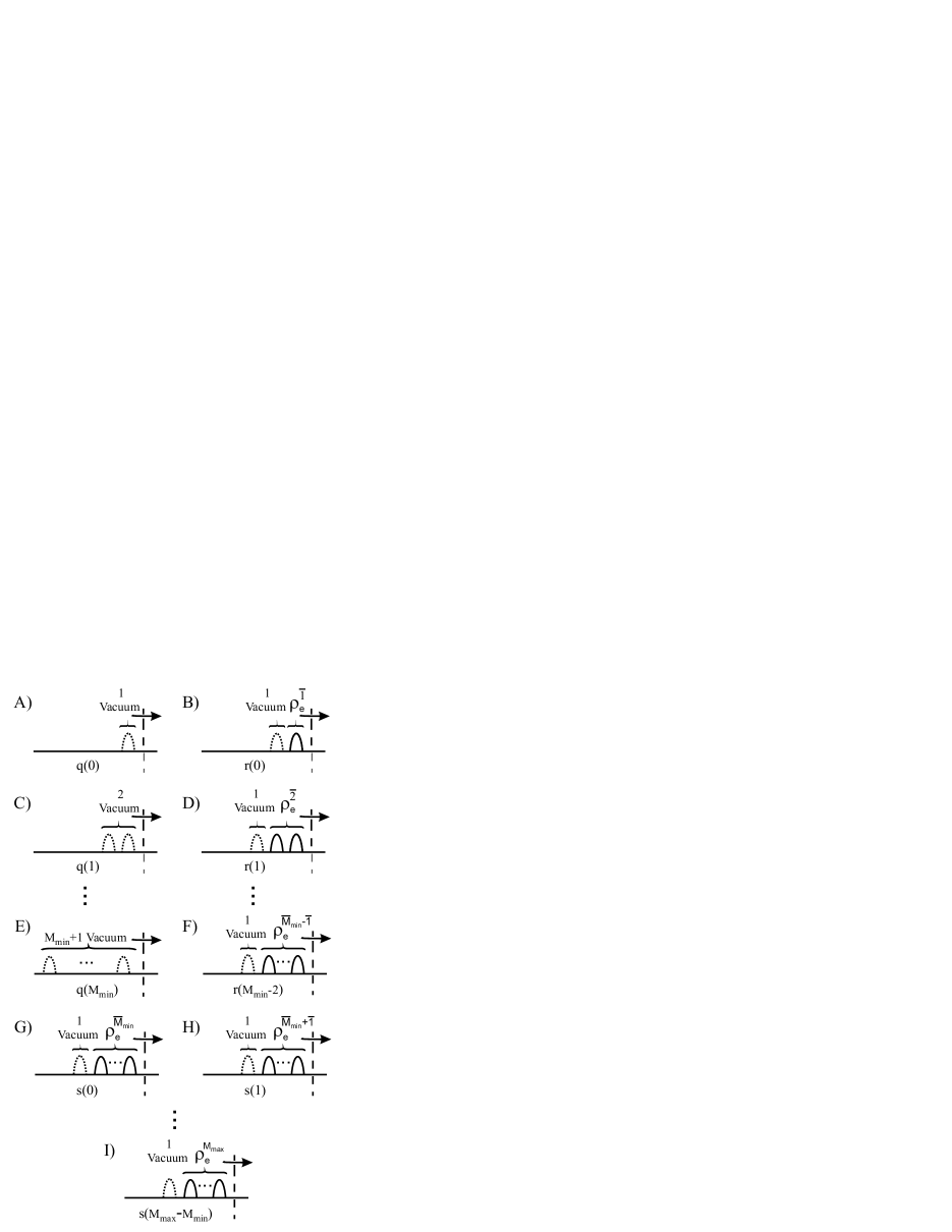
Figure 8: Possible signal states arriving at Bob’s detection apparatus after a dead-time, together with their a priori probabilities. The arrow indicates the transmission direction.

The superscript $\bar{k}$, with $1\leq{}\bar{k}<M_{max}$, that labels the states $\rho_{e}^{\bar{k}}$ in Fig. 8 is used to emphasize the fact that these signals may correspond to the last $\bar{k}$ temporal modes of any signal state $\rho_{e}^{k}$ with $k\geq{}\bar{k}$.

The parameters $N_{clicks}^{e}$ and $N^{e}$ can now be expressed, respectively, as

$$N_{clicks}^{e}=\sum_{m=1}^{\infty}p_{m}N_{clicks}^{e}(m),$$ (23)

where $N_{clicks}^{e}(m)$ denotes the average total number of clicks obtained by Bob when he receives the different blocks of signal states illustrated in Fig. 8 with $\rho_{e}^{\bar{k}}$ being the last $\bar{k}$ temporal modes of any state $|\psi_{k}^{m}\rangle$, and

$$N^{e}=\sum_{m=1}^{\infty}p_{m}N^{e}(m),$$ (24)

with $N^{e}(m)$ representing the average total number of pulses caused by these blocks of signal states. That is, to calculate $N^{e}(m)$ we need to consider not only the number of temporal modes contained in the signals illustrated in Fig. 8 but also the fact that whenever Bob obtains a click in any of these modes then he cannot obtain any other click during the following $\tilde{d}=\lceil{}t_{d}f_{c}\rceil$ pulses nsqp . The main idea behind the whole analysis contained in this section is to study the behaviour of the possible blocks of signals that Bob can receive from Eve after a dead-time, together with their a priori probabilities. Every time a dead-time finishes we have a new trial of this random process.

Next, we calculate an expression for $N_{clicks}^{e}(m)$ and $N^{e}(m)$. We shall distinguish several cases, depending on the block of signal states that arrives at Bob’s side after a dead-time. Let us begin with Case A in Fig. 8. The probability that Bob obtains a click in this scenario depends on the identity of the preceding signal. We shall denote with $p_{vv}$ the probability to obtain a click when the previous signal is also a vacuum state, and we shall denote with $p_{vk}^{m}$ the probability to obtain a click when the previous signal is the state $|\psi_{k}^{m}\rangle$. These two probabilities are calculated in Appendix D. In general, we have that $p_{vv}>0$ due to the dark counts in Bob’s detectors. Let $p_{pv}$ ($p_{pk}$) denote the probability that the previous signal is a vacuum state (the signal $|\psi_{k}^{m}\rangle$). These probabilities are calculated in Appendix E. With this notation, we find that the average total number of clicks in this scenario, that we shall represent as $N_{clicks,q(0)}^{e}(m)$, is given by

$$N_{clicks,q(0)}^{e}(m)=p_{pv}p_{vv}+\sum_{k=M_{min}}^{M_{max}}p_{pk}p_{vk}^{m}.$$ (25)

Next, we calculate an expression for the average total number of pulses, that we shall denote as $N^{e}_{q(0)}(m)$. This parameter depends on whether Bob’s detectors click or do not click. In particular, we have that whenever Bob obtains a click in his detection apparatus then the total number of pulses that we need to consider is $1+\tilde{d}$. That is, in this case we need to include the effect of the dead-time. Otherwise, the number of pulses is one. We obtain, therefore, that

$$N^{e}_{q(0)}(m) = p_{pv}[p_{vv}(1+\tilde{d})+(1-p_{vv})]$$

$$+ \sum_{k=M_{min}}^{M_{max}}p_{pk}[p_{vk}^{m}(1+\tilde{d})+(1-p_{vk}^{m})]$$

$$= p_{pv}(1+\tilde{d}p_{vv})+\sum_{k=M_{min}}^{M_{max}}p_{pk}(1+\tilde{d}p_{vk}^{m}).$$

The analysis of the remaining cases included in Fig. 8 is similar. Whenever Bob receives a block of $k+1$ vacuum states (Cases C and E in Fig. 8), with $1\leq{}k\leq{}M_{min}$, it is guaranteed that the signal which precedes the block is always a vacuum state. This is justified by the particular structure of the different blocks of signal states that Eve can send to Bob (see Fig. 2). In this case, due to the dead-time of Bob’s detectors, Bob can only obtain a click in a given temporal mode if the previous modes of the block did not click. The average total number of clicks, that we shall denote as $N_{clicks,q(k)}^{e}(m)$, can then be expressed as

$$N_{clicks,q(k)}^{e}(m)=\sum_{n=0}^{k}(1-p_{vv})^{n}{}p_{vv}=1-(1-p_{vv})^{k+1}.$$ (27)

In order to calculate the average total number of pulses, that we shall denote as $N^{e}_{q(k)}(m)$, note that, like before, whenever Bob obtains a click in temporal mode $l\in[0,k]$ then the total number of pulses that we need to consider is $(k-l)+(1+\tilde{d})$. The first term in the summation, $(k-l)$, represents the total number of modes contained in the block before the mode that actually clicked (see the labeling convention illustrated in Fig. 3), while the second term, $(1+\tilde{d})$, includes the effect of the dead-time. Otherwise, the number of pulses is $k+1$. We find, therefore, that $N^{e}_{q(k)}(m)$ can be written as

$$N^{e}_{q(k)}(m) = (k+1)(1-p_{vv})^{k+1}$$

$$+ \sum_{n=0}^{k}(n+1+\tilde{d})(1-p_{vv})^{n}p_{vv}$$

$$= \frac{(1+\tilde{d}p_{vv})\big{[}1-(1-p_{vv})^{k+1}\big{]}}{p_{vv}}.$$ (28)

When Bob receives a state $\rho_{e}^{\bar{k}}$, with $1\leq{}\bar{k}\leq{}M_{min}-1$, followed by one vacuum state (Cases B, D, and F in Fig. 8), then the state which precedes that block of signals can never be a vacuum state. Let $p_{\bar{k}}^{k}$ denote the probability that $\rho_{e}^{\bar{k}}$ stems from the last $\bar{k}$ temporal modes of a signal state $|\psi_{k}^{m}\rangle$ with $M_{min}\leq{}k\leq{}M_{max}$, and let $q_{\bar{k}}^{m}(k)$ be the average total number of clicks obtained by Bob in this scenario. The probability $p_{\bar{k}}^{k}$ is calculated in Appendix F, while the parameter $q_{\bar{k}}^{m}(k)$ can be written as

$$q_{\bar{k}}^{m}(k)=\sum_{n=0}^{\bar{k}}p_{c,\bar{k},k}^{m}(n),$$ (29)

with $p_{c,\bar{k},k}^{m}(n)$ denoting the probability that Bob obtains a click in temporal mode $n$ and he does not obtain a click in any previous mode $l$ with $n<l\leq{}\bar{k}$. This last quantity is calculated in Appendix D. With this notation, we have that the average total number of clicks in this case, that we shall denote as $N_{clicks,r(\bar{k}-1)}^{e}(m)$, can be expressed as

$$N_{clicks,r(\bar{k}-1)}^{e}(m)=\sum_{k=M_{min}}^{M_{max}}p_{\bar{k}}^{k}q_{\bar{k}}^{m}(k),$$ (30)

Similarly, the average total number of pulses has now the form

$$N^{e}_{r(\bar{k}-1)}(m)=\sum_{k=M_{min}}^{M_{max}}p_{\bar{k}}^{k}n_{\bar{k}}^{m}(k),$$ (31)

where the parameter $n_{\bar{k}}^{m}(k)$ represents the average total number of pulses when Bob receives the last $\bar{k}$ temporal modes of the signal $|\psi_{k}^{m}\rangle$ together with one vacuum state. This parameter is given by

$$n_{\bar{k}}^{m}(k) = \sum_{n=0}^{\bar{k}}p_{c,\bar{k},k}^{m}(n)[\bar{k}-n+1+\tilde{d}]$$

$$+ [1-q_{\bar{k}}^{m}(k)](1+\bar{k}).$$ (32)

Bob can receive as well a state $\rho_{e}^{\bar{k}}$, with $M_{min}\leq{}\bar{k}\leq{}M_{max}$, followed by one vacuum state (Cases G, H and I in Fig. 8). Let $p_{pv\bar{k}}$ denote the probability that the preceding signal is a vacuum state, and let $p_{p\bar{k}}^{k}$ be the probability that $\rho_{e}^{\bar{k}}$ stems from the last $\bar{k}$ temporal modes of the signal state $|\psi_{k}^{m}\rangle$, with $\bar{k}<k\leq{}M_{max}$. These two probabilities are calculated in Appendix G. Using this notation, we obtain that the average total number of clicks in this scenario, that we shall denote as $N_{clicks,s(\bar{k}-M_{min})}^{e}(m)$, with $M_{min}\leq{}\bar{k}\leq{}M_{max}$, can be expressed as

$$N_{clicks,s(\bar{k}-M_{min})}^{e}(m)=p_{pv\bar{k}}q_{\bar{k}}^{m}(\bar{k})+\sum_{k=\bar{k}+1}^{M_{max}}p_{p\bar{k}}^{k}q_{\bar{k}}^{m}(k),$$ (33)

while the average total number of pulses, that we shall denote as $N_{s(\bar{k}-M_{min})}^{e}(m)$, can directly be obtained from Eq. (33) just by substituting the parameters $q_{\bar{k}}^{m}(k)$, with $\bar{k}\leq{}k\leq{}M_{max}$, by $n_{\bar{k}}^{m}(k)$.

Finally, $N_{clicks}^{e}(m)$ and $N^{e}(m)$ can be calculated by adding all these terms together with their a priori probabilities. That is,

$$N_{clicks}^{e}(m) = \sum_{k=0}^{M_{min}}q(k)N_{clicks,q(k)}^{e}(m)$$

$$+ \sum_{k=0}^{M_{min}-2}r(k)N_{clicks,r(k)}^{e}(m)$$

$$+ \sum_{k=0}^{M_{max}-M_{min}}s(k)N_{clicks,s(k)}^{e}(m),$$ (34)

and similarly for $N^{e}(m)$.

V.2 Quantum bit error rate

The QBER in this strategy is given by Eq. (14), with the parameter $N_{clicks}^{e}$ now given by Eq. (23). In order to obtain $N_{errors}^{e}$ we follow the same method like in the previous section. In particular, this quantity can now be expressed as

$$N_{errors}^{e}=\sum_{m=1}^{\infty}p_{m}N_{errors}^{e}(m),$$ (35)

where $N_{errors}^{e}(m)$ denotes the average total number of errors obtained by Bob when he receives from Eve the different blocks of signal states illustrated in Fig. 8 with $\rho_{e}^{\bar{k}}$ representing the last $\bar{k}$ temporal modes of any state $|\psi_{k}^{m}\rangle$ with $k\geq{}\bar{k}$. Note, moreover, that in this scenario vacuum states can also produce errors in Bob’s detection apparatus due to the dark counts.

The analysis to obtain the parameter $N_{errors}^{e}(m)$ is completely equivalent to the one included in Sec. V.1 to calculate $N_{clicks}^{e}(m)$; basically one only needs to substitute Bob’s probabilities to obtain a click $p_{vv}$, $p_{vk}^{m}$, and $p_{c,\bar{k},k}^{m}(n)$ by the probabilities to obtain an error in precisely the same situations when these probabilities were introduced. For instance, we need to substitute $p_{vv}$ by the probability that Bob obtains an error when he receives from Eve a vacuum state and the preceding signal is also a vacuum state, and similar for the other cases. These error probabilities, that we shall denote, respectively, as $e_{vv}$, $e_{vk}^{m}$, and $p_{e,\bar{k},k}^{m}(n)$ are calculated in Appendix H. The only exception is the parameter $N_{errors,q(k)}^{e}(m)$ (Cases C and E in Fig. 8), with $1\leq{}k\leq{}M_{min}$. This exception only arises due to the notation used in Sec. V.1. Bob can obtain an error in a given temporal mode $n+1$ if the previous modes of the block did not clicked; that is, the probability to have an error in that mode is $(1-p_{vv})^{n}{}e_{vv}$. We obtain, therefore, that $N_{errors,q(k)}^{e}(m)$ is now given by

$$N_{errors,q(k)}^{e}(m) = \sum_{n=0}^{k}(1-p_{vv})^{n}{}e_{vv}$$

$$= e_{vv}+e_{vv}\frac{1-p_{vv}}{p_{vv}}\big{[}1-(1-p_{vv})^{k}\big{]}.$$

V.3 Double click rate

So far we have considered the case of the standard DPS QKD protocol, where only the raw bit rate, together with the time slots in which Bob obtains a click, are monitored. In this section, however, we briefly analyze the case of an extended version of the protocol, where Alice and Bob can also make use of the double click rate at Bob’s side to try to detect Eve. That is, every time Bob obtains a double click in his detection apparatus he first records this event and, afterwards, he selects randomly the bit value. This is motivated by the fact that, unlike the type of signal states considered in Sec. IV, now the states $\rho_{e}^{k}$ given by Eq. (20) always present a non vanishing probability of producing a double click. This means, in particular, that Alice and Bob could employ this information to discard those sequential attacks that increase the double click rate that they expect due to the statistical fluctuations in the channel, together with the effect of dark counts in Bob’s detectors dcr_uds .

The double click rate at Bob’s side, that we shall denote as $D_{c}$, is typically defined as $D_{c}=N_{D_{c}}/N$, where $N_{D_{c}}$ refers to the average total number of double clicks obtained by Bob, and $N$ is again the total number of signal states sent by Alice. $N_{D_{c}}$ can be expressed as $N_{D_{c}}=(N/N^{e})N_{D_{c}}^{e}$, with $N^{e}$ given by Eq. (24) and where $N_{D_{c}}^{e}$ denotes the average total number of double clicks obtained by Bob when he receives from Eve the different blocks of signals illustrated in Fig. 8. With this notation, we find that $D_{c}$ can be written as

$$D_{c}=\frac{N_{D_{c}}^{e}}{N^{e}}.$$ (37)

The parameter $N_{D_{c}}^{e}$ can be expressed as

$$N_{D_{c}}^{e}=\sum_{m=1}^{\infty}p_{m}N_{D_{c}}^{e}(m),$$ (38)

where $N_{D_{c}}^{e}(m)$ denotes the average total number of double clicks obtained by Bob when the signal states $\rho_{e}^{\bar{k}}$ illustrated in Fig. 8 represent the last $\bar{k}$ temporal modes of any state $|\psi_{k}^{m}\rangle$.

Again, the analysis to obtain $N_{D_{c}}^{e}(m)$ is completely equivalent to the one included in Sec. V.1 to calculate $N_{clicks}^{e}(m)$. We only need to substitute in Eq. (V.1) the probabilities to obtain a click $p_{vv}$, $p_{vk}^{m}$, and $p_{c,\bar{k},k}^{m}(n)$ by the probabilities to obtain a double click in the same situation. We shall denote these double click probabilities as $dc_{vv}$, $dc_{vk}^{m}$ and $p_{dc,\bar{k},k}^{m}(n)$, and they are calculated in Appendix I. The only exception is the parameter $N_{D_{c},q(k)}^{e}(m)$ (Cases C and E in Fig. 8), with $1\leq{}k\leq{}M_{min}$. The reason for this exception is similar to the one presented in Sec. V.2 for the parameter $N_{errors,q(k)}^{e}(m)$. In particular, $N_{D_{c},q(k)}^{e}(m)$ can be obtained from Eq. (V.2) by substituting the probability $e_{vv}$ by $dc_{vv}$.

V.4 Evaluation

In Figs. 9, 10, 11 and 12 we plot the gain $G$ versus the QBER in a sequential attack for different values of the mean photon number $\mu_{\alpha}$ of Alice’s signal states, the parameter $\tilde{d}$, the dark count probability $p_{d}$ and the detection efficiency $\eta_{det}$ of Bob’s detectors, and the photon number $m$ of Eve’s signal states dete_effi . These examples illustrate the case of the standard DPS QKD protocol where Alice and Bob do not monitor separately the double click rate at Bob’s side and Eve can select the parameter $m$ without any restriction on the maximum tolerable double click rate. As before, these figures state that the secret key rate above the curves is zero.

Figure 9: Gain ($G$) versus QBER in a sequential attack for different values of the photon number $m$, and for the optimal distribution of the state coefficients $A_{n,m}^{(k)}$ derived in Sec. IV. The mean photon number of Alice’s signal states is $\mu_{\alpha}=0.2$, the parameter $\tilde{d}=500$, the dark count probability of Bob’s detectors is $p_{d}=2.5\times{}10^{-9}$, and the detection efficiency $\eta_{det}=0.005$. The triangles represent experimental data from Ref. dpsqkd_exp3 .

Figure 10: Gain ($G$) versus QBER in a sequential attack for different values of the photon number $m$, and for the optimal distribution of the state coefficients $A_{n,m}^{(k)}$ derived in Sec. IV. The mean photon number of Alice’s signal states is $\mu_{\alpha}=0.17$, the parameter $\tilde{d}=50$, the dark count probability of Bob’s detectors is $p_{d}=7.8\times{}10^{-6}$, and the detection efficiency $\eta_{det}=0.0327$. The triangle represents experimental data from Ref. dpsqkd_exp1 . (See also Ref. dpsqkd_exp2b .)

Figure 11: Gain ($G$) versus QBER in a sequential attack for different values of the photon number $m$, and for the optimal distribution of the state coefficients $A_{n,m}^{(k)}$ derived in Sec. IV. The mean photon number of Alice’s signal states is $\mu_{\alpha}=0.16$, the parameter $\tilde{d}=50$, the dark count probability of Bob’s detectors is $p_{d}=2.7\times{}10^{-7}$, and the detection efficiency $\eta_{det}=0.0045$. The triangle represents experimental data from Ref. dpsqkd_exp1 . (See also Ref. dpsqkd_exp2b .)

Figure 12: Gain ($G$) versus QBER in a sequential attack for different values of the photon number $m$, and for the optimal distribution of the state coefficients $A_{n,m}^{(k)}$ derived in Sec. IV. The mean photon number of Alice’s signal states is $\mu_{\alpha}=0.2$, the parameter $\tilde{d}=50$, the dark count probability of Bob’s detectors is $p_{d}=3.5\times{}10^{-8}$, and the detection efficiency $\eta_{det}=0.0011$. The triangles represent experimental data from Ref. dpsqkd_exp2 . (See also Ref. dpsqkd_exp2b .)

We fix the value of $M_{max}=\tilde{d}$ and we vary the value of the parameters $M_{min}<M_{max}$ and $q\in[0,1]$ like in Sec. IV.3. Moreover, for simplicity, we select the state coefficients $A_{n,m}^{(k)}$ of the signal states $\rho^{k}_{e}$ given by Eq. (20) as $A_{n,m}^{(k)}=A_{n}^{(k)}$ for all $m\geq{}1$, with $A_{n}^{(k)}$ given by the optimal distribution derived in Appendix B for the case of the untrusted device scenario. It can be shown that also in this case this distribution provides a lower QBER than the one obtained with a flat or a binomial distribution. As expected, the QBER produced by a sequential attack starts decreasing as the losses in the channel increase, and, at some point, it begins to increase again. This inflexion point is due to the dark count probability of Bob’s detectors, which Eve cannot manipulate in the trusted device scenario. In particular, when the gain is low enough such that most of the clicks obtained by Bob originate from the dark counts of his detectors then the QBER starts increasing again. In the limit case where all the detected events arise from dark counts we have that the QBER=0.5. Figs. 9, 10, 11 and 12 also include experimental data from Refs. dpsqkd_exp1 ; dpsqkd_exp2 ; dpsqkd_exp2b ; dpsqkd_exp3 . According to our results, and for the values of the parameter $m$ considered in these examples, we find that the $200$ km DPS QKD experiment reported in Ref. dpsqkd_exp3 together with the $105$ km DPS QKD experiment reported in Ref. dpsqkd_exp1 would be insecure against a sequential attack even in the trusted device scenario. That is, the data of these experiments could never be turned into secret key.

As already suggested in Ref. curty_dps , in this QKD protocol it is not enough for Alice and Bob to include the effect of the double clicks obtained by Bob in the QBER, but it might be very useful for the legitimate users to monitor also the double click rate to guarantee security against a sequential attack. Fig. 13 shows a graphical representation of the gain versus the double click rate for the case where $\mu_{\alpha}=0.17$, $\tilde{d}=50$, $p_{d}=7.8\times{}10^{-6}$, $\eta_{det}=0.0327$, and for different values of the parameter $m$ dpsqkd_exp1 . (See also Ref. dpsqkd_exp2b .) Similar results can also be obtained for the experimental parameters used in Refs. dpsqkd_exp2 ; dpsqkd_exp3 . As expected, the double click rate at Bob’s side decreases as the losses in the channel increases and the photon number $m$ decreases. If Alice and Bob only accept a double click rate below the curve which corresponds to the case $m=1$ then they could always detect the sequential attacks presented in this section.

Figure 13: Gain ($G$) versus double click rate ($D_{c}$) in a sequential attack for different values of the photon number $m$, and for the optimal distribution of the state coefficients $A_{n,m}^{(k)}$ derived in Sec. IV. The experimental parameters coincide with those used in Fig. 10.

VI CONCLUSION

In this paper we have quantitatively analyzed the effect that Bob’s detectors dead-time has on the performance of sequential attacks against a differential-phase-shift (DPS) quantum key distribution (QKD) protocol based on weak coherent pulses. A sequential attack consists of Eve measuring out every coherent state emitted by Alice and, afterwards, she prepares new signal states, depending on the results obtained, that are given to Bob. Whenever Eve obtains a predetermined number of consecutive successful measurement outcomes, then she prepares a new train of non-vacuum signal states that is forwarded to Bob. Otherwise, Eve can send vacuum signals to Bob to avoid errors. Sequential attacks transform the original quantum channel between Alice and Bob into an entanglement breaking channel and, therefore, they do not allow the distribution of quantum correlations needed to establish a secret key.

Specifically, we have studied sequential attacks where Eve realizes unambiguous state discrimination of Alice’s signal states. When Eve identifies unambiguously a signal state sent by Alice, then she considers this result as successful. Otherwise, she considers it as a failure. Moreover, we have considered two possible scenarios for our analysis. In the first one, so-called untrusted device scenario, we assumed that Eve can control some imperfections in Alice and Bob’s devices (e.g., the detection efficiency, the dark count probability, and the dead-time of Bob’s detectors), together with the quantum channel, and she exploits them to obtain maximal information about the shared key. In the second scenario, so-called trusted device scenario, we considered that Eve cannot modify the actual detection devices employed by Alice and Bob. That is, the legitimate users have complete knowledge about their detectors, which are fixed by the actual experiment. From a practical point of view, this last case constitutes a reasonable description of a realistic situation, where Alice and Bob could in principle try to limit Eve’s influence on their apparatus by some counterattack techniques.

As a result, we obtained upper bounds on the maximal distance achievable by a DPS QKD scheme as a function of the error rate in the sifted key, and the detection efficiency, the dark count probability, and the dead-time of Bob’s detectors. It states that no key distillation protocol can provide a secret key from the correlations established by the users. While our analysis seems to indicate that in the untrusted device scenario all the long-distance implementations of DPS QKD reported so far in the literature would be insecure against a sequential attack, it also suggests that, in the trusted device scenario, it might be very useful for the legitimate users to monitor also the double click rate at Bob’s side. This fact might dramatically increase Alice and Bob’s ability in defeating sequential attacks in this case.

VII ACKNOWLEDGEMENTS

The authors wish to thank Norbert Lütkenhaus, Bing Qi and especially Hoi-Kwong Lo for very fruitful discussions on the topic of this paper and very useful comments on the manuscript. Financial support from DFG under the Emmy Noether programme, and the European Commission (Integrated Project SECOQC) are gratefully acknowledged. This research was supported in part by Perimeter Institute for Theoretical Physics. Research at Perimeter Institute is supported in part by the Government of Canada through NSERC and by the province of Ontario through MEDT. M.C. and K.T. would like to thank Hoi-Kwong Lo for hospitality and support during their stays at the University of Toronto. K.T. also thanks the National Institute of Information and Communications Technology, in Japan, for the support.

Appendix A Average total number of errors $e(k)$

In this appendix we obtain an expression for the average total number of errors $e(k)$ obtained by Bob when Eve sends him a signal state $|\psi_{e}^{k}\rangle$ followed by $1+d$ vacuum states (Cases A, B, and C in Fig. 2). These signal states always produce one single click in Bob’s detection apparatus and, therefore, they can cause at most one single error (i.e., $e(k)\leq{}1$). This error can occur in any temporal mode $n\in[0,k]$. The parameter $e(k)$ can be written as

$$e(k)=\sum_{n=0}^{k}p_{err}^{k,n},$$ (39)

where $p_{err}^{k,n}$ denotes the probability that Bob obtains an error in temporal mode $n$. Next, we calculate this probability.

We shall consider that Bob employs the detection setup shown in Fig. 1. We will assume as well that his detectors, $D0$ and $D1$, have a detection efficiency equal to one, a dark count probability equal to zero, and they cannot distinguish the number of photons of arrival signals. That is, they provide only two possible outcomes: “click” (at least one photon is detected), and “no click” (no photon is detected in the pulse). The action of $D0$ and $D1$ in the time slot $n$ can be characterized by one positive operator value measure (POVM) that contains four elements: $D_{vac}^{n}$, $D_{0}^{n}$, $D_{1}^{n}$, and $D_{Dc}^{n}$. The outcome of the first operator $D_{vac}^{n}$ corresponds to no click in the detectors, the following POVM operator $D_{0}^{n}$ ($D_{1}^{n}$) gives precisely one detection click in detector $D0$ ($D1$), and the last one $D_{Dc}^{n}$ gives rise to both detectors being triggered. If we denote by $\mbox{$|p,q\rangle$}_{D0,D1}^{n}$ the state that, in temporal mode $n$, contains $p$ photons in the spatial mode arriving to detector $D0$ and $q$ photons in the spatial mode corresponding to detector $D1$, then the elements of this POVM can be expressed as

$$D_{vac}^{n}=\mbox{$|0,0\rangle$}\mbox{$\langle 0,0|$}^{n}_{D0,D1}$$

$$D_{0}^{n}=\sum_{p=1}^{\infty}\mbox{$|p,0\rangle$}\mbox{$\langle p,0|$}^{n}_{D0,D1}$$

$$D_{1}^{n}=\sum_{p=1}^{\infty}\mbox{$|0,p\rangle$}\mbox{$\langle 0,p|$}^{n}_{D0,D1}$$

$$D_{Dc}^{n}=\sum_{p,q=1}^{\infty}\mbox{$|p,q\rangle$}\mbox{$\langle p,q|$}^{n}_{D0,D1}$$ (40)

Once the state $|\psi_{e}^{k}\rangle$ followed by $1+d$ vacuum states passes Bob’s interferometer, the signal that arrives at Bob’s detectors, that we shall denote as $|\tilde{\psi}_{e}^{k}\rangle$, is given by

$$\mbox{$|\tilde{\psi}_{e}^{k}\rangle$}=\sum_{n=1}^{k}B_{n}^{(k)}\big{[}\hat{a}_{n,D0}^{\dagger}-\hat{a}_{n,D1}^{\dagger}+\hat{a}_{n-1,D0}^{\dagger}+\hat{a}_{n-1,D1}^{\dagger}\big{]}\mbox{$|0\rangle$}$$ (41)

followed by $d$ vacuum states. The coefficients $B_{n}^{(k)}$ in Eq. (41) are given by $B_{n}^{(k)}=[A_{n}^{(k)}\exp{(i\theta_{n})}]/2$, and $\hat{a}_{n,D0}^{\dagger}$ ($\hat{a}_{n,D1}^{\dagger}$) represents a creation operator for one photon in temporal mode $n$ and in the spatial mode corresponding to detector $D0$ ($D1$).

It turns out that the probability $p_{err}^{k,n}$ remains constant independently of the different possible combinations of correct phases $\theta_{n}$ identified by Eve. Therefore, without loss of generality, we can assume a fixed value for the angles $\theta_{n}$. In particular, we shall consider, for instance, that $\theta_{n}=0$ for all $n\in[1,k]$ and, consequently, $B_{n}^{(k)}=A_{n}^{(k)}/2$. In this scenario an error occurs when detector $D1$ clicks. The probability $p_{err}^{k,n}$ can then be expressed as $p_{err}^{k,n}=\text{Tr}(D_{1}^{n}\mbox{$|\tilde{\psi}_{e}^{k}\rangle$}\mbox{$\langle\tilde{\psi}_{e}^{k}|$})$, with $|\tilde{\psi}_{e}^{k}\rangle$ given by Eq. (41). As a result, we obtain

$$p_{err}^{k,k} = \frac{1}{4}|{}A_{k}^{(k)}|{}^{2}$$

$$p_{err}^{k,0<n<k} = \frac{1}{4}|{}A_{n+1}^{(k)}-A_{n}^{(k)}|{}^{2}$$

$$p_{err}^{k,0} = \frac{1}{4}|{}A_{1}^{(k)}|{}^{2}.$$ (42)

Adding all these terms together according to Eq. (39) we finally obtain

$$e(k)=\frac{1}{4}\Bigg{[}|{}A_{1}^{(k)}|{}^{2}+\sum_{n=1}^{k-1}|{}A_{n+1}^{(k)}-A_{n}^{(k)}|{}^{2}+|{}A_{k}^{(k)}|{}^{2}\Bigg{]}.$$ (43)

Appendix B Optimization of $A_{n}^{(k)}$

In this appendix we describe a method to optimize the state coefficients $A_{n}^{(k)}$ introduced in Eq. (4) for the untrusted device scenario. As shown in Sec. IV.1, in this case the overall gain $G$ is independent of the chosen distribution for these coefficients. This means that the minimum value of the QBER can be attained by optimizing the average total number of errors $e(k)$ independently of $G$.

The coefficients $A_{n}^{(k)}\in\mathbb{C}$ satisfy the normalization condition $\sum_{n=1}^{k}|{}A_{n}^{(k)}|{}^{2}=1$. In polar coordinates each of these coefficients can be expressed as $A_{n}^{(k)}=a^{(k)}_{n}\exp(i\psi^{(k)}_{n})$, with $a^{(k)}_{n}$, and $\psi^{(k)}_{n}\in\mathbb{R}$. With this notation, the terms $|A_{n+1}^{(k)}-A_{n}^{(k)}|^{2}$ in Eq. (16) simplify to

$$|A_{n+1}^{(k)}-A_{n}^{(k)}|^{2} = (a^{(k)}_{n+1})^{2}+(a^{(k)}_{n})^{2}$$ (44)

$$- 2a^{(k)}_{n}a^{(k)}_{n+1}\cos(\psi^{(k)}_{n+1}-\psi^{(k)}_{n})$$

$$\geq (a^{(k)}_{n+1}-a^{(k)}_{n})^{2},$$

where equality is obtained iff $\psi^{(k)}_{n+1}-\psi^{(k)}_{n}$ is an even multiple of $\pi$, i.e., both $A_{n+1}^{(k)}$ and $A_{n}^{(k)}$ have the same phase. Then, without loss of generality, we can always impose the phases $\psi^{(k)}_{n}$, with $n\in[1,k]$, to be equal to zero. With this constraint, together with the normalization condition of the state coefficients, one can further simplify the parameters $e(k)$ as

$$e(k)=\frac{1}{2}\left(1-\sum_{n=1}^{k-1}a_{n+1}^{(k)}a_{n}^{(k)}\right).$$ (45)

Now, in order to minimize this quantity one can equivalently solve the following optimization problem,

minimize $$c\sum_{n=1}^{k}(a_{n}^{(k)})^{2}-\sum_{n=1}^{k-1}a_{n+1}^{(k)}a_{n}^{(k)}$$

subject to $$\sum_{n=1}^{k}(a_{n}^{(k)})^{2}=1,$$ (46)

where $c>0$ is an arbitrary positive constant. This optimization problem can be written in matrix form as

$$\text{minimize}_{\|\vec{a}_{k}\|=1}f(\vec{a}_{k})=\vec{a}_{k}M(c)\vec{a}_{k}^{T},$$ (47)

where the vector $\vec{a}_{k}$ is defined as $\vec{a}_{k}=(a_{1}^{(k)},\dots,a_{k}^{(k)})$, and the matrix $M(c)=c\openone-K/2$ with $K=K^{T}$ being a $k\times k$ matrix with ones only on the first off-diagonals and zeros elsewhere, i.e.,

$$K=\left(\begin{array}[]{ccccccc}0&1&0&\ldots\\ 1&0&1&\ldots\\ 0&1&0&\ldots\\ \vdots&\vdots&\vdots&\ddots\end{array}\right).$$ (48)

The Hessian matrix of the function $f(\vec{a}_{k})$ is $M(c)$; hence if one selects the constant $c$ such that $M(c)>0$ then the resulting optimization problem is convex, and it suffices to find a local minimum. The solution is given by

$$\text{minimize}_{\|\vec{a}_{k}\|=1}f(\vec{a}_{k}) = c-\text{maximize}_{\|\vec{a}_{k}\|=1}\vec{a}_{k}K\vec{a}_{k}$$ (49)

$$= c-\lambda_{max}(K),$$

where $\lambda_{max}(K)$ denotes the maximal eigenvalue of the matrix $K$. The optimal solution for the state coefficients $A_{n}^{(k)}$ coincides then with the elements of the normalized eigenvector of $K$ that is associated with its maximal eigenvalue.

Fig. 14 shows a graphical representation of $e(k)$ versus $k$ for the optimal distribution of $A_{n}^{(k)}$ together with the flat and the binomial distributions given in Eq. (IV.3).

Figure 14: The average total number of errors $e(k)$ versus $k$ for different distributions of the state coefficients $A_{n}^{(k)}$: flat (solid), binomial (dashed), and the optimal distribution (dotted).

Appendix C Probabilities $q(k)$, $r(k)$ and $s(k)$

In this appendix we provide the expressions for the a priori probabilities of the blocks of signal states illustrated in Fig. 8: $q(k)$, $r(k)$ and $s(k)$. As already explained in Sec. V, these blocks of signal states arise due to the effect of the dead-time of Bob’s detectors. In particular, in the trusted device scenario it is not guaranteed that the first temporal mode that arrives at Bob’s side once his detectors are recovered from a dead-time coincides with the first temporal mode of any of the blocks of signals considered in Fig. 2. In this scenario, and for a given block of signals containing $k+1$ modes (see Fig. 2), we shall denote with $p_{d}(n)$ the probability that the first temporal mode of the block that arrives at Bob’s side after a dead-time is mode $k-n$. That is, $p_{d}(n)$ represents the probability that a dead-time finishes once Bob has already received the first $n$ temporal modes of a given block of signals. For instance, $p_{d}(0)$ represents the probability that the first mode that arrives at Bob’s side after a dead-time coincides with the first temporal mode of the block, $p_{d}(1)$ denotes the probability that the first mode arriving at Bob’s side corresponds to the second temporal mode of the block, and so on. Here we use again the labeling convention illustrated in Fig. 3.

With this notation, let us now calculate the parameter $q(0)$, i.e., the probability that Bob receives a vacuum state after a dead-time (Case A in Fig. 8). In principle, this vacuum state could originate from the last temporal mode of every block of signal states illustrated in Fig. 2 with $d=0$. For instance, the probability that it originates from the block of signals which contains only one vacuum state (Case D in Fig. 2 when the parameter $k=0$) is given by $p_{d}(0)p_{v}(0)$, where $p_{v}(0)$ is given by Eq. (3). In general, we have that the probability that this vacuum state arises from a block of signals which contains $k+1$ vacuum states, with $0\leq{}k\leq{}M_{min}$ (Cases D and E in Fig. 2), is given by $p_{d}(k)p_{v}(k)/[\sum_{m=n-k}^{M_{min}}p_{v}(m)+\sum_{m^{\prime}=M_{min}}^{M_{max}}p_{s}(m^{\prime})]$, where the normalization factor $\sum_{m=n-k}^{M_{min}}p_{v}(m)+\sum_{m^{\prime}=M_{min}}^{M_{max}}p_{s}(m^{\prime})$ is used to guarantee that, for each value of the parameter $p_{d}(n)$, the probabilities of the different blocks of signal states which contain at least $n+1$ temporal modes add one. Similarly, we find that the probability that this vacuum state originates from a block of signals containing a state $\rho_{e}^{k}$ followed by one vacuum state, with $M_{min}\leq{}k\leq{}M_{max}$ (Cases A, B, and C in Fig. 2 with $d=0$), can be written as $p_{d}(k)p_{s}(k)/\{\sum_{m=k}^{M_{max}}[p_{v}(m)+p_{s}(m)]\}$. After adding all these terms together, we obtain that $q(0)$ can be expressed as

$$q(0) = \sum_{n=0}^{M_{min}}\frac{p_{d}(n)p_{v}(n)}{1-\sum_{m=0}^{n-1}p_{v}(m)}$$

$$+ \sum_{k=M_{min}}^{M_{max}}\frac{p_{d}(k)p_{s}(k)}{\sum_{m=k}^{M_{max}}\big{[}p_{v}(m)+p_{s}(m)\big{]}}$$ (50)

The analysis of the remaining cases is completely analogous. In particular, we find that

$$q(k)=\sum_{n=k}^{M_{min}}\frac{p_{d}(n-k)p_{v}(n)}{1-\sum_{m=0}^{n-1-k}p_{v}(m)},$$ (51)

with $1\leq{}k\leq{}M_{min}$,

$$r(k)=\sum_{n=M_{min}}^{M_{max}}\frac{p_{d}(n-1-k)p_{s}(n)}{\sum_{m=n-1-k}^{M_{max}}\big{[}p_{v}(m)+p_{s}(m)\big{]}},$$ (52)

with $0\leq{}k\leq{}M_{min}-2$, and

$$s(k)=\sum_{n=M_{min}+k}^{M_{max}}\frac{p_{d}(n-M_{min}-k)p_{s}(n)}{\sum_{m=n-M_{min}-k}^{M_{max}}\big{[}p_{v}(m)+p_{s}(m)\big{]}},$$ (53)

with $0\leq{}k\leq{}M_{max}-M_{min}$.

To conclude, let us present very briefly a numerical method to calculate the probabilities $p_{d}(n)$, with $0\leq{}n\leq{}M_{max}$. This procedure is used in Sec. V.4 for the graphical representation of the gain $G$ versus the QBER (and also of the double click rate versus $G$) in a sequential attack. For simplicity, let us consider the situation where $M_{max}=\lceil{}t_{d}f_{c}\rceil$. That is, each block of signal states illustrated in Fig. 8 could produce, at most, only one single click in Bob’s detectors due to the effect of the dead-time. In this scenario, the probabilities $p_{d}(n)$ only depend on whether the previous $M_{max}+1$ temporal modes which precede a block of signals clicked or did not click. Especifically, we have that $p_{d}(0)$ is given by the probability that none of these $M_{max}+1$ previous modes clicked or it only clicked the first of them. That is,

$$p_{d}(0)=G+(1-G)^{M_{max}+1}.$$ (54)

Similarly, $p_{d}(n)$, with $1\leq{}n\leq{}M_{max}$, can be expressed as

$$p_{d}(n)=G(1-G)^{n}.$$ (55)

Then, in order to obtain $p_{d}(n)$ an plot the figures included in Sec. V.4, we perform several iterations for each value of the gain $G$. First, we calculate the probabilities $p_{d}(n)$ according to Eq. (54) and Eq. (55) and, with these probabilities, we obtain a new value for the gain $G$. We repeat this procedure several times until the value of $G$ converges to a constant value.

Appendix D Probabilities $p_{vv}$, $p_{vk}^{m}$ and $p_{c,\bar{k},k}^{m}(n)$

In this appendix we obtain an expression for the probabilities of obtaining a click at Bob’s side: $p_{vv}$, $p_{vk}^{m}$ and $p_{c,\bar{k},k}^{m}(n)$, introduced in Sec. V.1.

Let us start by describing Bob’s detectors $D0$ and $D1$ in the trusted device scenario. As already introduced in Sec. V, these detectors are characterized by their detection efficiency $\eta_{det}$, their dark count probability $p_{d}$, and their dead-time. The detection efficiency of $D0$ and $D1$ can be modeled by a combination of beam splitters of transmittance $\eta_{det}$ and ideal detectors yurke_85 . This model can be simplified further by considering that both detectors have the same detection efficiency. In this situation, it is possible to attribute the losses of both detectors to a single-loss beam splitter which is located after the transmission channel. Moreover, like in Sec. IV, we shall assume that $D0$ and $D1$ cannot distinguish the number of photons of arrival signals, but they provide only as possible outcomes “click” and “no click”. This means, in particular, that the action of Bob’s ideal detectors can be characterized by the POVM given by Eq. (A). Furthermore, the noise introduced by $D0$ and $D1$ due to their dark counts can be considered to be independent of the incoming signals. Note that the clicks that Bob observes can be thought as coming from a two-step process: in the first step the signal states sent by Eve can produce clicks in his detectors, while in the second step random clicks from the detector’s dark counts is added.

Next, we calculate an expression for the probability $p_{c,\bar{k},k}^{m}(n)$. For that, we obtain first the probability that Bob’s detectors fire due to the signal states sent by Eve only, i.e., without taking into account the dark counts of $D0$ and $D1$; afterwards we will include in the analysis the effect of the dark counts of the detectors.

Once a state $|\psi_{k}^{m}\rangle$, followed by one vacuum state, passes Bob’s interferometer together with the beam splitter which models the losses of his detectors, the signal that arrives at Bob’s ideal detectors, that we shall denote as $|\tilde{\psi}_{k}^{m}\rangle$, is given by

$$\mbox{$|\tilde{\psi}_{k}^{m}\rangle$}=\frac{1}{\sqrt{m!}}\Big{[}\sum_{n=0}^{k}(E_{n}^{m}\hat{a}_{n,D1}^{\dagger}+F_{n}^{m}\hat{a}_{n,D0}^{\dagger})+\sum_{n=1}^{k}G_{n}^{m}\hat{b}_{n}^{\dagger}\Big{]}^{m}\mbox{$|0\rangle$},$$ (56)

where $\hat{a}_{n,D0}^{\dagger}$ ($\hat{a}_{n,D1}^{\dagger}$) represents again a creation operator for one photon in temporal mode $n$ and in the spatial mode arriving to detector $D0$ ($D1$), $\hat{b}_{n}^{\dagger}$ denotes a creation operator for one photon in temporal mode $n$ and in the spatial mode that goes out of the beam splitter that models the losses of the detectors, and the coefficients $E_{n}^{m}$, $F_{n}^{m}$, and $G_{n}^{m}$ are given by

$$E_{n}^{m}=\left\{\begin{array}[]{ll}\eta A_{1,m}^{(k)}e^{i\theta_{1}}&\textrm{if $n=0$}\\ \eta[A_{n+1,m}^{(k)}e^{i\theta_{n+1}}-A_{n,m}^{(k)}e^{i\theta_{n}}]&\textrm{if $1\leq{}n\leq{}k-1$}\\ -\eta A_{k,m}^{(k)}e^{i\theta_{k}}&\textrm{if $n=k$},\\ \end{array}\right.$$ (57)

with $\eta=\sqrt{\eta_{det}}/2$,

$$F_{n}^{m}=\left\{\begin{array}[]{ll}\eta A_{1,m}^{(k)}e^{i\theta_{1}}&\textrm{if $n=0$}\\ \eta[A_{n+1,m}^{(k)}e^{i\theta_{n+1}}+A_{n,m}^{(k)}e^{i\theta_{n}}]&\textrm{if $1\leq{}n\leq{}k-1$}\\ \eta A_{k,m}^{(k)}e^{i\theta_{k}}&\textrm{if $n=k$},\\ \end{array}\right.$$ (58)

and

$$G_{n}^{m}=\sqrt{1-\eta_{det}}A_{n,m}^{(k)}e^{i\theta_{n}},$$ (59)

respectively.

Let $p_{c,\bar{k},k}^{m,s}(n)$ denote the probability that Bob obtains a click in mode $n$, with $0\leq{}n\leq{}\bar{k}$, and he does not obtain a click in any previous temporal mode $l$, with $n<l\leq{}\bar{k}$, when he receives the last $\bar{k}$ temporal modes of a signal state $|\psi_{k}^{m}\rangle$ followed by one vacuum state. This probability can be expressed as

$$p_{c,\bar{k},k}^{m,s}(n)=p_{\bar{k},k,D0}^{m}(n)+p_{\bar{k},k,D1}^{m}(n)+p_{\bar{k},k,D_{Dc}}^{m}(n),$$ (60)

where $p_{\bar{k},k,D0}^{m}(n)$ ($p_{\bar{k},k,D1}^{m}(n)$) represents the probability that only detector $D0$ ($D1$) clicks in temporal mode $n$, and $p_{\bar{k},k,D_{Dc}}^{m}(n)$ denotes the probability that both detectors $D0$ and $D1$ click in temporal mode $n$ nuevotexto . These probabilities are given by

$$p_{\bar{k},k,Di}^{m}(n)=\text{Tr}\bigg{(}\bigotimes_{l=n+1}^{\bar{k}}D_{vac}^{l}\otimes{}D_{i}^{n}\mbox{$|\tilde{\psi}_{k}^{m}\rangle$}\mbox{$\langle\tilde{\psi}_{k}^{m}|$}\bigg{)},$$ (61)

where the POVM elements $D_{vac}^{l}$ and $D_{i}^{n}$, with $i\in{}\{0,1,D_{c}\}$, are given by Eq. (A). After some calculations, we obtain that these probabilities can be written, respectively, as

$$p_{\bar{k},k,D0}^{m}(n) = \sum_{\begin{subarray}{c}\sum_{\begin{subarray}{c}r=0\\ r\notin{}I_{0}\end{subarray}}^{3k+1}t_{r}=m\\ t_{(k+n+1)}\geq{}1\end{subarray}}\frac{m!}{\prod_{\begin{subarray}{c}l=0\\ l\notin{}I_{0}\end{subarray}}^{3k+1}t_{l}!}\prod_{\begin{subarray}{c}i=0\\ i\notin{}[n,\bar{k}]\end{subarray}}^{k}|{}E_{i}^{m}|{}^{2t_{i}}$$

$$\times \prod_{\begin{subarray}{c}j=0\\ j\notin{}[n+1,\bar{k}]\end{subarray}}^{k}|{}F_{j}^{m}|{}^{2t_{(j+k+1)}}\prod_{s=1}^{k}|{}G_{s}^{m}|{}^{2t_{(s+2k+1)}},$$

$$p_{\bar{k},k,D1}^{m}(n) = \sum_{\begin{subarray}{c}\sum_{\begin{subarray}{c}r=0\\ r\notin{}I_{1}\end{subarray}}^{3k+1}t_{r}=m\\ t_{n}\geq{}1\end{subarray}}\frac{m!}{\prod_{\begin{subarray}{c}l=0\\ l\notin{}I_{1}\end{subarray}}^{3k+1}t_{l}!}\prod_{\begin{subarray}{c}i=0\\ i\notin{}[n+1,\bar{k}]\end{subarray}}^{k}|{}E_{i}^{m}|{}^{2t_{i}}$$

$$\times \prod_{\begin{subarray}{c}j=0\\ j\notin{}[n,\bar{k}]\end{subarray}}^{k}|{}F_{j}^{m}|{}^{2t_{(j+k+1)}}\prod_{s=1}^{k}|{}G_{s}^{m}|{}^{2t_{(s+2k+1)}},$$

$$p_{\bar{k},k,D_{Dc}}^{m}(n) = \sum_{\begin{subarray}{c}\sum_{\begin{subarray}{c}r=0\\ r\notin{}I_{Dc}\end{subarray}}^{3k+1}t_{r}=m\\ t_{(k+n+1)}\geq{}1\\ t_{n}\geq{}1\end{subarray}}\frac{m!}{\prod_{\begin{subarray}{c}l=0\\ l\notin{}I_{Dc}\end{subarray}}^{3k+1}t_{l}!}\prod_{\begin{subarray}{c}i=0\\ i\notin{}[n+1,\bar{k}]\end{subarray}}^{k}\big{[}|{}E_{i}^{m}|{}^{t_{i}}$$

$$\times |{}F_{i}^{m}|{}^{t_{(i+k+1)}}\big{]}^{2}\prod_{s=1}^{k}|{}G_{s}^{m}|{}^{2t_{(s+2k+1)}},$$ (62)

where the sets of indexes $I_{0}$, $I_{1}$ and $I_{Dc}$ are given by: $I_{0}=[n,\bar{k}]\cup[n+k+2,\bar{k}+k+1]$, $I_{1}=[n+1,\bar{k}]\cup[n+k+1,\bar{k}+k+1]$ and $I_{Dc}=[n+1,\bar{k}]\cup[n+k+2,\bar{k}+k+1]$. It turns out that the probability $p_{c,\bar{k},k}^{m,s}(n)$ remains invariable independently of the different possible combinations of correct consecutive phases $\theta_{n}$ identified by Eve. Therefore, without loss of generality, we can always assume a fixed value for the angles $\theta_{n}$; for instance, we can consider that $\theta_{n}=0$ for all $n\in[1,k]$. This means, in particular, that the parameters $E_{n}^{m}$, $F_{n}^{m}$ and $G_{n}^{m}$ that appear in Eq. (D) depend only on the state coefficients $A_{n,m}^{(k)}$ and the detection efficiency of Bob’s detectors.

In order to include the effect of the dark counts of $D0$ and $D1$ in the analysis, let us define the parameter $P_{d}$ as

$$P_{d}=p_{d}(2-p_{d}).$$ (63)

This is the probability to have a click at Bob’s side in a given time slot due to the dark counts of his detectors only. As already mentioned in Sec. V.1, here we consider that double click events are not discarded by Bob. Every time Bob obtains a double click, he just decides randomly the bit value Norbert99 . With this notation, it turns out that the probability that Bob obtains a click in temporal mode $n$, with $0\leq{}n\leq{}\bar{k}$, and he does not obtain a click in any previous mode $l$, with $n<l\leq{}\bar{k}$, due to the dark counts of his detectors only, probability that we shall denote as $p_{c,\bar{k}}^{m,d}(n)$, is given by

$$p_{c,\bar{k}}^{m,d}(n)=P_{d}(1-P_{d})^{\bar{k}-n}.$$ (64)

Combining Eq. (60) and Eq. (64), we obtain that the probability $p_{c,\bar{k},k}^{m}(n)$ can be expressed as

$$p_{c,\bar{k},k}^{m}(n) = p_{c,\bar{k},k}^{m,s}(n)(1-P_{d})^{\bar{k}-n+1}+p_{c,\bar{k}}^{m,d}(n)$$ (65)

$$\times p_{\bar{k},k,D_{vac}}^{m}(n)+p_{c,\bar{k},k}^{m,s}(n)p_{c,\bar{k}}^{m,d}(n)$$

$$= p_{c,\bar{k},k}^{m,s}(n)(1-P_{d})^{\bar{k}-n}+p_{c,\bar{k}}^{m,d}(n)p_{\bar{k},k,D_{vac}}^{m}(n),$$

where $p_{\bar{k},k,D_{vac}}^{m}(n)$ is given by Eq. (61) with $D_{i}=D_{vac}$, i.e., it represents the probability that Bob does not obtain a click in any temporal mode $l$, with $n\leq{}l\leq{}\bar{k}$, due to the signals sent by Eve only. This probability can be written as

$$p_{\bar{k},k,D_{vac}}^{m}(n) = \sum_{\begin{subarray}{c}\sum_{\begin{subarray}{c}r=0\\ r\notin{}I_{vac}\end{subarray}}^{3k+1}t_{r}=m\end{subarray}}\frac{m!}{\prod_{\begin{subarray}{c}l=0\\ l\notin{}I_{vac}\end{subarray}}^{3k+1}t_{l}!}\prod_{\begin{subarray}{c}i=0\\ i\notin{}[n,\bar{k}]\end{subarray}}^{k}\big{[}|{}E_{i}^{m}|{}^{t_{i}}$$

$$\times |{}F_{i}^{m}|{}^{t_{(i+k+1)}}\big{]}^{2}\prod_{s=1}^{k}|{}G_{s}^{m}|{}^{2t_{(s+2k+1)}},$$ (66)

with the set $I_{vac}=[n,\bar{k}]\cup[n+k+1,\bar{k}+k+1]$.

Finally, we obtain an expression for the probabilities $p_{vv}$ and $p_{vk}^{m}$. The first one, $p_{vv}$, represents the probability that Bob obtains a click when he receives a vacuum state and the preceding signal is also a vacuum state. This probability has the form $p_{vv}=P_{d}$, where $P_{d}$ is given by Eq. (63). Similarly, $p_{vk}^{m}$ denotes the probability that Bob obtains a click when he receives a vacuum state and the preceding signal is the state $|\psi_{k}^{m}\rangle$. This probability is given by $p_{vk}^{m}=p_{c,0,k}^{m}(0)$, where $p_{c,\bar{k},k}^{m}(n)$ is defined in Eq. (65).

Appendix E Probabilities $p_{pv}$ and $p_{pk}$

In this appendix we obtain an expression for the probabilities $p_{pv}$ and $p_{pk}$. Let us begin with $p_{pv}$, i.e., the probability that the signal which precedes a vacuum state (Case A in Fig. 8) is also a vacuum state.

As shown in Appendix C, after a dead-time Bob receives a vacuum state with a probability given by Eq. (C). The first summation in Eq. (C) refers to the probability that this vacuum state originates from a block of signal states containing only vacuum pulses (Cases D and E in Fig. 2). We have, therefore, that $p_{pv}$ can be written as

$$p_{pv}=\frac{1}{q(0)}\sum_{n=0}^{M_{min}}\frac{p_{d}(n)p_{v}(n)}{1-\sum_{m=0}^{n-1}p_{v}(m)},$$ (67)

where the normalization factor $q(0)$ is used to guarantee that $p_{pv}+\sum_{M_{min}}^{M_{max}}p_{pk}=1$. Similarly, each term $p_{d}(k)p_{s}(k)/\sum_{m=k}^{M_{max}}\big{[}p_{v}(m)+p_{s}(m)\big{]}$ that appears in the second summation of Eq. (C) represents the probability that Bob receives a vacuum state preceded by a signal $|\psi_{k}^{m}\rangle$ (Cases A, B and C in Fig. 2 when the number of photons contained in $\rho_{e}^{k}$ is equal to $m$). After normalizing by the factor $q(0)$ we find that $p_{pk}$ is given by

$$p_{pk}=\frac{p_{d}(k)p_{s}(k)}{q(0)\sum_{m=k}^{M_{max}}\big{[}p_{v}(m)+p_{s}(m)\big{]}},$$ (68)

with $M_{min}\leq{}k\leq{}M_{max}$.

Appendix F Probability $p^{k}_{\bar{k}}$

In this appendix we calculate the probability $p^{k}_{\bar{k}}$ with $1\leq{}\bar{k}\leq{}M_{min}-1$, i.e., the probability that $\rho_{e}^{\bar{k}}$ represents the last $\bar{k}$ temporal modes of a signal state $|\psi_{k}^{m}\rangle$ with $M_{min}\leq{}k\leq{}M_{max}$ (Cases B, D, and F in Fig. 8).

As shown in Appendix C, after a dead-time Bob receives the signal $\rho_{e}^{\bar{k}}$ followed by one vacuum state with probability $r(\bar{k}-1)$, where the probability $r(k)$ is given by Eq. (52). Each term $p_{d}(n-1-l)p_{s}(n)/\sum_{m=n-1-l}^{M_{max}}[p_{v}(m)+p_{s}(m)]$ that appears in the summation of Eq. (52) denotes the probability that Bob receives a state $\rho_{e}^{l+1}$ which corresponds to the last $l+1$ temporal modes of a signal $|\psi_{n}^{m}\rangle$. After substituting $l+1=\bar{k}$ and $n=k$, and normalizing by the factor $r(\bar{k}-1)$ we find that $p^{k}_{\bar{k}}$ is given by

$$p_{\bar{k}}^{k}=\frac{p_{d}(k-\bar{k})p_{s}(k)}{r(\bar{k}-1)\sum_{m=k-\bar{k}}^{M_{max}}[p_{v}(m)+p_{s}(m)]}.$$ (69)

Appendix G Probabilities $p_{pv\bar{k}}$ and $p_{p\bar{k}}^{k}$

In this appendix we obtain an expression for the probabilities $p_{pv\bar{k}}$ and $p_{p\bar{k}}^{k}$, i.e., the probability that the signal state $\rho_{e}^{\bar{k}}$ received by Bob, with $M_{min}\leq{}\bar{k}\leq{}M_{max}$, is preceded by a vacuum state, and the probability that $\rho_{e}^{\bar{k}}$ represents the last $\bar{k}$ temporal modes of $|\psi_{k}^{m}\rangle$, with $\bar{k}<k\leq{}M_{max}$, respectively (Cases G, H and I in Fig. 8).

As shown in Appendix C, after a dead-time Bob receives the signal state $\rho_{e}^{\bar{k}}$ with a probability given by Eq. (53). This probability can be equivalently written as

$$s(\bar{k}-M_{min})=\sum_{n=\bar{k}}^{M_{max}}\frac{p_{d}(n-\bar{k})p_{s}(n)}{\sum_{m=n-\bar{k}}^{M_{max}}\big{[}p_{v}(m)+p_{s}(m)\big{]}},$$ (70)

with $M_{min}\leq{}\bar{k}\leq{}M_{max}$. The first term in the summation given by Eq. (70), i.e, the case $n=\bar{k}$, refers to the probability that Bob receives a state $\rho_{e}^{\bar{k}}=\mbox{$|\psi_{\bar{k}}^{m}\rangle$}\mbox{$\langle\psi_{\bar{k}}^{m}|$}$. Because of the particular structure of the blocks of signal states that Eve can send to Bob (see Fig. 2), these states are always preceded by a vacuum state. After normalizing by the factor $s(\bar{k}-M_{min})$ we obtain, therefore, that $p_{pv\bar{k}}$ is given by

$$p_{pv\bar{k}}=\frac{p_{d}(0)p_{s}(\bar{k})}{s(\bar{k}-M_{min})}.$$ (71)

Similarly, each term $p_{d}(n-\bar{k})p_{s}(n)/\sum_{m=n-\bar{k}}^{M_{max}}[p_{v}(m)+p_{s}(m)]$ that appears in Eq. (70), with $\bar{k}<n\leq{}M_{max}$, represents the probability that Bob receives a state $\rho_{e}^{\bar{k}}$ which originates from the signal state $|\psi_{n}^{m}\rangle$. We find, therefore, that

$$p_{p\bar{k}}^{k}=\frac{p_{d}(k-\bar{k})p_{s}(k)}{s(\bar{k}-M_{min})\sum_{n=k-\bar{k}}^{M_{max}}[p_{v}(n)+p_{s}(n)]}.$$ (72)

The normalization factor $s(\bar{k}-M_{min})$ included in Eq. (71) and in Eq. (72) guarantees that $p_{pv\bar{k}}+\sum_{k=\bar{k}+1}^{M_{max}}p_{p\bar{k}}^{k}=1$.

Appendix H Probabilities $e_{vv}$, $e_{vk}^{m}$ and $p_{e,\bar{k},k}^{m}(n)$

In this appendix we obtain an expression for the error probabilities $e_{vv}$, $e_{vk}^{m}$, and $p_{e,\bar{k},k}^{m}(n)$ introduced in Sec. V.2.

Let us start with the parameter $e_{vv}$, i.e., the probability that Bob obtains an error when he receives from Eve a vacuum state and the preceding signal is also a vacuum state. This quantity is given by $e_{vv}=p_{d}(1-p_{d})+p_{d}^{2}/2$, where $p_{d}$ denotes the dark count probability of Bob’s detectors. This quantity can be further simplified as

$$e_{vv}=\frac{1}{2}P_{d},$$ (73)

with $P_{d}$ given by Eq. (63).

The parameter $p_{e,\bar{k},k}^{m}(n)$, i.e., the probability that Bob obtains an error in temporal mode $n$ and he does not obtain a click in any previous temporal mode $l$, with $n<l\leq{}\bar{k}$, when he receives the last $\bar{k}$ temporal modes of the signal $|\psi_{k}^{m}\rangle$ followed by one vacuum state can be calculated as the probability that Bob obtains a click in the “wrong” detector and no click in the “correct” one, together with one half the probability that he obtains a double click. Like in Sec. IV.2, the total error probability in this strategy remains invariant independently of the different possible combinations of correct phases $\theta_{n}$ identified by Eve. For simplicity, therefore, we can consider again that all these phases are equal to zero. This means, in particular, that in this situation the “wrong” detector corresponds to detector $D1$. The probability $p_{e,\bar{k},k}^{m}(n)$ can then be expressed as $p_{e,\bar{k},k}^{m}(n)=[p_{\bar{k},k,D1}^{m}(n)+p_{\bar{k},k,D_{Dc}}^{m}(n)/2](1-P_{d})^{\bar{k}-n+1}+p_{\bar{k},k,D_{vac}}^{m}(n)(1-P_{d})^{\bar{k}-n}P_{d}/2+[p_{\bar{k},k,D1}^{m}(n)/2+p_{\bar{k},k,D_{Dc}}^{m}(n)/2](1-P_{d})^{\bar{k}-n}p_{d}(1-p_{d})+[p_{\bar{k},k,D0}^{m}(n)/2+p_{\bar{k},k,D_{Dc}}^{m}(n)/2+p_{\bar{k},k,D1}^{m}(n)](1-P_{d})^{\bar{k}-n}p_{d}(1-p_{d})+[p_{\bar{k},k,D0}^{m}(n)+p_{\bar{k},k,D1}^{m}(n)+p_{\bar{k},k,D_{Dc}}^{m}(n)](1-P_{d})^{\bar{k}-n}p_{d}^{2}/2$, where the parameters $p_{\bar{k},k,D0}^{m}(n)$, $p_{\bar{k},k,D1}^{m}(n)$ and $p_{\bar{k},k,D_{Dc}}^{m}(n)$ are given by Eq. (D), and $p_{\bar{k},k,D_{vac}}^{m}(n)$ is given by Eq. (D). This quantity can be further simplified as

$$p_{e,\bar{k},k}^{m}(n) = (1-P_{d})^{\bar{k}-n}\bigg{[}\bigg{(}1-\frac{p_{d}}{2}\bigg{)}p_{\bar{k},k,D1}^{m}(n)$$

$$+ \frac{p_{d}p_{\bar{k},k,D0}^{m}(n)}{2}+\frac{p_{\bar{k},k,D_{Dc}}^{m}(n)}{2}$$

$$+ p_{d}\bigg{(}1-\frac{p_{d}}{2}\bigg{)}p_{\bar{k},k,D_{vac}}^{m}(n)\bigg{]}.$$ (74)

Similarly, the parameter $e_{vk}^{m}$, i.e., the probability that Bob obtains an error when he receives a vacuum state and the preceding signal is the state $|\psi_{k}^{m}\rangle$ has the form $e_{vk}^{m}=p_{e,0,k}^{m}(0)$, with $p_{e,\bar{k},k}^{m}(n)$ given by Eq. (H).

Appendix I Probabilities $dc_{vv}$, $dc_{vk}^{m}$ and $p_{dc,\bar{k},k}^{m}(n)$

In this appendix we obtain an expression for the double click probabilities $dc_{vv}$, $dc_{vk}^{m}$ and $p_{dc,\bar{k},k}^{m}(n)$ introduced in Sec. V.3.

The probability $dc_{vv}$, i.e., the probability that Bob obtains a double click when he receives from Eve a vacuum state and the preceding signal is also a vacuum state is given by

$$dc_{vv}=p_{d}^{2},$$ (75)

where $p_{d}$ denotes again the dark count probability of Bob’s detectors.

The parameter $p_{dc,\bar{k},k}^{m}(n)$, i.e., the probability that Bob obtains a double click in temporal mode $n$ and he does not obtain a click in any previous temporal mode $l$, with $n<l\leq{}\bar{k}$, when he receives the last $\bar{k}$ temporal modes of the signal $|\psi_{k}^{m}\rangle$ followed by one vacuum state is given by $p_{dc,\bar{k},k}^{m}(n)=p_{\bar{k},k,D_{Dc}}^{m}(n)(1-P_{d})^{\bar{k}-n+1}+p_{\bar{k},k,D_{vac}}^{m}(n)(1-P_{d})^{\bar{k}-n}p_{d}^{2}+[p_{\bar{k},k,D1}^{m}(n)+p_{\bar{k},k,D_{Dc}}^{m}(n)](1-P_{d})^{\bar{k}-n}p_{d}(1-p_{d})+[p_{\bar{k},k,D0}^{m}(n)+p_{\bar{k},k,D_{Dc}}^{m}(n)](1-P_{d})^{\bar{k}-n}p_{d}(1-p_{d})+[p_{\bar{k},k,D0}^{m}(n)+p_{\bar{k},k,D1}^{m}(n)+p_{\bar{k},k,D_{Dc}}^{m}(n)](1-P_{d})^{\bar{k}-n}p_{d}^{2}$. This quantity can be further simplified as

$$p_{dc,\bar{k},k}^{m}(n) = (1-P_{d})^{\bar{k}-n}\bigg{\{}p_{d}\big{[}p_{\bar{k},k,D1}^{m}(n)+p_{\bar{k},k,D0}^{m}(n)\big{]}$$

$$+ p_{\bar{k},k,D_{Dc}}^{m}(n)+p_{d}^{2}p_{\bar{k},k,D_{vac}}^{m}(n)\bigg{\}}.$$ (76)

Finally, the parameter $dc_{vk}^{m}$, i.e., the probability that Bob obtains a double click when he receives a vacuum state and the preceding signal is the state $|\psi_{k}^{m}\rangle$ has the form $dc_{vk}^{m}=p_{dc,0,k}^{m}(0)$, with $p_{dc,\bar{k},k}^{m}(n)$ given by Eq. (I).

References

- (1) N. Gisin, G. Ribordy, W. Tittel and H. Zbinden, Rev. Mod. Phys. 74, 145 (2002); M. Dušek, N. Lütkenhaus and M. Hendrych, Progress in Optics 49, Edt. E. Wolf (Elsevier), 381 (2006).
- (2) G. S. Vernam, Trans. of the AIEE 45, 295 (1926).
- (3) C. H. Bennett and G. Brassard, Proc. IEEE Int. Conference on Computers, Systems and Signal Processing, Bangalore, India, IEEE Press, New York, 175 (1984).
- (4) D. Mayers, J. of ACM 48, 351 (2001); H.-K. Lo and H. F. Chau, Science 283, 2050 (1999); E. Biham, M. Boyer, P. O. Boykin, T. Mor and V. Roychowdhury, Proc. of the Thirty Second Annual ACM Symposium on Theory of Computing, New York, USA, ACM Press, New York, 715 (2000); P. W. Shor and J. Preskill, Phys. Rev. Lett. 85, 441 (2000).
- (5) C. H. Bennett, F. Bessette, G. Brassard, L. Salvail and J. Smolin, J. Cryptology 5, 3 (1992).
- (6) C. Marand and P. D. Townsend, Opt. Lett. 20, 1695 (1995); D. S. Bethune, M. Navarro and W. P. Risk, Applied Opt. LP 41, 1640 (2002); R. J. Hughes, J. E. Nordholt, D. Derkacs and C. G. Peterson, New J. Phys. 4, 43 (2002); D. Stucki, N. Gisin, O. Guinnard, G. Ribordy and H. Zbinden, New J. Phys. 4, 41 (2002); C. Gobby, Z. L. Yuan and A. J. Shields, Appl. Phys. Lett. 84, 3762 (2004); C. Gobby, Z. L. Yuan and A. J. Shields, Electron. Lett. 40, 1603 (2004).
- (7) B. Huttner, N. Imoto, N. Gisin and T. Mor, Phys. Rev. A 51, 1863 (1995).
- (8) G. Brassard, N. Lütkenhaus, T. Mor and B. C. Sanders, Phys. Rev. Lett. 85, 1330 (2000).
- (9) N. Lütkenhaus, Phys. Rev. A 61, 052304 (2000).
- (10) H. Inamori, N. Lütkenhaus and D. Mayers, Eur. Phys. J. D 41, 599 (2007).
- (11) D. Gottesman, H.-K. Lo, N. Lütkenhaus and J. Preskill, Quant. Inf. Comp. 4, 325 (2004).
- (12) W.-Y. Hwang, Phys. Rev. Lett. 91, 057901 (2003); H.-K. Lo, X. Ma and K. Chen, Phys. Rev. Lett. 94, 230504 (2005); X.-B. Wang, Phys. Rev. Lett. 94, 230503 (2005); X. Ma, B. Qi, Y. Zhao and H.-K. Lo, Phys. Rev. A. 72, 012326 (2005); X.-B. Wang, Phys. Rev. A 72, 012322 (2005); X.-B. Wang, Phys. Rev. A 72, 049908 (2005); J. W. Harrington, J. M. Ettinger, R. J. Hughes and J. E. Nordholt, Los Alamos report LA-UR-05-1156 (2005), quant-ph/0503002; X. Ma, C.-H. F. Fung, F. Dupuis, K. Chen, K. Tamaki and H.-K. Lo, Phys. Rev. A 74, 032330 (2006); X.-B. Wang, C.-Z. Peng and J.-W. Pan, Appl. Phys. Lett. 90, 031110 (2007); X.-B. Wang, Phys. Rev. A 75, 052301 (2007); W. Mauerer and C. Silberhorn, Phys. Rev. A 75, 050305 (2007).
- (13) Y. Zhao, B. Qi, X. Ma, H.-K. Lo and L. Qian, Phys. Rev. Lett. 96, 070502 (2006); Y. Zhao, B. Qi, X. Ma, H.-K. Lo and L. Qian, Proc. of IEEE International Symposium on Information Theory (ISIT’06), 2094 (2006); C.-Z. Peng, J. Zhang, D. Yang, W.-B. Gao, H.-X. Ma, H. Yin, H.-P. Zeng, T. Yang, X.-B. Wang and J.-W. Pan, Phys. Rev. Lett. 98, 010505 (2007); D. Rosenberg, J. W. Harrington, P. R. Rice, P. A. Hiskett, C. G. Peterson, R. J. Hughes, A. E. Lita, S. W. Nam and J. E. Nordholt, Phys. Rev. Lett. 98, 010503 (2007); T. Schmitt-Manderbach, H. Weier, M. Fürst, R. Ursin, F. Tiefenbacher, T. Scheidl, J. Perdigues, Z. Sodnik, C. Kurtsiefer, J. G. Rarity, A. Zeilinger and H. Weinfurter, Phys. Rev. Lett. 98, 010504 (2007); Z. L. Yuan, A. W. Sharpe and A. J. Shields, Appl. Phys. Lett. 90, 011118 (2007); Z.-Q. Yin, Z.-F. Han, W. Chen, F.-X. Xu, Q.-L. Wu and G.-C. Guo, quant-ph/0704.2941; J. Hasegawa, M. Hayashi, T. Hiroshima, A. Tanaka and A. Tomita, quant-ph/0705.3081; J. F. Dynes, Z. L. Yuan, A. W. Sharpe and A. J. Shields, Optics Express 15, 8465 (2007).
- (14) C. H. Bennett, Phys. Rev. Lett. 68, 3121 (1992).
- (15) M. Koashi, Phys. Rev. Lett. 93, 120501 (2004); K. Tamaki, N. Lütkenhaus, M. Koashi and J. Batuwantudawe, quant-ph/0607082.
- (16) K. Inoue, E. Waks and Y. Yamamoto, Phys. Rev. Lett. 89, 037902 (2002); K. Inoue, E. Waks and Y. Yamamoto, Phys. Rev. A 68, 022317 (2003).
- (17) E. Waks, H. Takesue and Y. Yamamoto, Phys. Rev. A 73, 012344 (2006).
- (18) H. Takesue, E. Diamanti, T. Honjo, C. Langrock, M. M. Fejer, K. Inoue and Y. Yamamoto, New J. Phys. 7, 232 (2005).
- (19) E. Diamanti, H. Takesue, C. Langrock, M. M. Fejer and Y. Yamamoto, Opt. Express 14, 13073 (2006).
- (20) E. Diamanti, Ph.D Thesis, Stanford University (2006).
- (21) H. Takesue, S. W. Nam, Q. Zhang, R. H. Hadfield, T. Honjo, K. Tamaki and Y. Yamamoto, Nature Photonics 1, 343 (2007).
- (22) C. Branciard, N. Gisin and V. Scarani, New J. Phys. 10, 013031 (2008).
- (23) M. Curty, L.L. Zhang, H.-K. Lo and N. Lütkenhaus, Quant. Inf. Comp. 7, 665 (2007).
- (24) T. Tsurumaru, Phys. Rev. A 75, 062319 (2007).
- (25) M. Duek, M. Jahma and N. Lütkenhaus, Phys. Rev. A 62, 022306 (2000).
- (26) S. Félix, N. Gisin, A. Stefanov and H. Zbinden, J. Mod. Opt. 48, 2009 (2001).
- (27) M. Curty and N. Lütkenhaus, Phys. Rev. A 71, 062301 (2005).
- (28) M. Curty, M. Lewenstein and N. Lütkenhaus, Phys. Rev. Lett. 92, 217903 (2004); M. Curty, O. Gühne, M. Lewenstein and N. Lütkenhaus, Phys. Rev. A 71, 022306 (2005).
- (29) In order to simplify our notation, from now on we will employ the term “signal state” only to denote those light pulses with a mean photon number bigger than zero. A light pulse with an average photon number equal to zero will be always denoted as a “vacuum state”.
- (30) I. D. Ivanovic, Phys. Lett. A 123, 257 (1987); D. Dieks, Phys. Lett. A 126, 303 (1988); A. Peres, Phys. Lett. A 128, 19 (1988); G. Jaeger and A. Shimony, Phys. Lett. A 197, 83 (1995).
- (31) A. Chefles and S. M. Barnett, Phys. Lett. A 250, 223 (1998).
- (32) For instance, any attempt by Eve to shift the wavelength of the signals into a region of a higher detection efficiency of Bob’s detectors can be blocked by the use of a narrow frequency filter.
- (33) D. Stucki, N. Brunner, N. Gisin, V. Scarani and H. Zbinden, Appl. Phys. Lett. 87, 194108 (2005).
- (34) N. Gisin, G. Ribordy, H. Zbinden, D. Stucki, N. Brunner and V. Scarani, quant-ph/0411022 (2004).
- (35) C. Branciard, N. Gisin, N. Lütkenhaus and V. Scarani, Quant. Inf. Comp. 7, 639 (2007).
- (36) M. Horodecki, P. W. Shor and M. B. Ruskai, Rev. Math. Phys. 15, 629 (2003); M. B. Ruskai, Rev. Math. Phys. 15, 643 (2003).
- (37) In order to show that Eve can always phase-lock her local oscillator to the coherent light source of Alice note that she could employ, for instance, the following recursive method. First, she uses a beam splitter to extract a portion of light of several (say ) consecutive signal states emitted by Alice. Afterwards, she continues splitting more times this pulses that she has just extracted. As a result, she obtains trains of pulses each. These pulses maintain the same phase relationship as the original ones sent by Alice. Now, she measures out the first train of pulses by using the same detection apparatus like Bob. With some finite probability she can identify the relative phase of some pairs of consecutive pulses inside this train. Once this process ends, Eve discards, from the remaining trains of signals, those pairs of pulses whose relative phase was not unambiguously determined on the first train. Finally, she combines the remaining pairs using a beam splitter. This way, Eve can obtain new trains of pulses containing a smaller number of them. Most importantly, since Eve knows the relative phase of each pair of pulses that entered the beam splitter in the previous step, and as a result of this, she knows in which output port of it she has a pulse of coherent light. This means, in particular, that the amplitudes of these new coherent pulses contained in the new trains are also amplified. Eve repeats this procedure several times on these remaining trains of signals, i.e., she measures out the first of these trains by using again the same detection device like Bob, and then she follows the same steps described above. As a result, and assuming that and are large enough, Eve can obtain a very bright single pulse and she can measure its phase.
- (38) This measurement strategy is very similar to the one considered in Ref. curty_dps . Note, however, that it provides Eve with a higher success probability of unambiguously identifying a sequence of signal states. The reason for this is that in Ref. curty_dps Eve first divides her data of measurement outcomes into different blocks of the same length and, afterwards, she analyzes each block of data independently, i.e., without considering the data included in adjacent blocks. Therefore, in this scenario it may happen that two consecutive blocks do not contain enough successful USD outcomes to consider their sequences of measurement results successful unless the data included in both blocks is jointly evaluated.
- (39) Note that Bob can also obtain a click in temporal mode due to the time delay introduced by Bob’s interferometer in one of its paths.
- (40) M. Curty and N. Lütkenhaus, Phys. Rev. A 69, 042321 (2004).
-
(41)
Since in DPS QKD Bob does not monitor the coherence
between states with different photon number, there is no difference for Eve whether she sends
to Bob the signal states given by
Eq. (20), or she sends him the signal states
with given by Eq. (21).(77) - (42) N. Lütkenhaus, Applied Phys. B 69, 395 (1999).
- (43) In this section we shall use the parameter defined as instead of the parameter employed in Sec. IV. The main motivation for this change of the notation is to try to avoid ambiguities when referring to the parameter . In particular, since in the trusted device scenario we impose for the blocks of signal states illustrated in Fig. 2.
- (44) In this extended version of the DPS QKD protocol Alice and Bob could as well employ the double click rate information that is measured in the experiment to try to discard those sequential attacks that highly decrease the value of the double click rate expected by the legitimate users. For instance, we have shown in Sec. IV that the eavesdropping strategy employed by Eve in the untrusted device scenario produces a double click rate equal to zero. However, if we consider a real implementation of the protocol, then this last scenario is not so simple, since the double click rate expected by Alice and Bob due to the dark counts of the detectors is usually quite low.
- (45) In this section we consider that the parameter also includes the losses due to Bob’s interferometer.
- (46) B. Yurke, Phys. Rev. A 32, 311 (1985).
- (47) Note that in this definition we treat double clicks like single click events.