Fluctuations in Mass-Action Equilibrium of Protein Binding Networks

Abstract

We consider two types of fluctuations in the mass-action equilibrium in protein binding networks. The first type is driven by relatively slow changes in total concentrations (copy numbers) of interacting proteins. The second type, to which we refer to as spontaneous, is caused by quickly decaying thermodynamic deviations away from the equilibrium of the system. As such they are amenable to methods of equilibrium statistical mechanics used in our study. We investigate the effects of network connectivity on these fluctuations and compare them to their upper and lower bounds. The collective effects are shown to sometimes lead to large power-law distributed amplification of spontaneous fluctuations as compared to the expectation for isolated dimers. As a consequence of this, the strength of both types of fluctuations is positively correlated with the overall network connectivity of proteins forming the complex. On the other hand, the relative amplitude of fluctuations is negatively correlated with the abundance of the complex. Our general findings are illustrated using a real network of protein-protein interactions in baker s yeast with experimentally determined protein concentrations.

The study of dynamical fluctuations in complex systems has emerged as a topic of intense interest germane to the fields of biology Bio_fluct , financial systems Finance_fluct , traffic in information Traffic_info_fluct and transportation Traffic_trans_fluct networks, and many others. Of particular interest is the nature of collective effects that arise as a consequence of the connectivity of the underlying network. By examining such fluctuations we can understand when the underlying network plays an important role and when, if possible, it may be ignored. A good candidate arena to study dynamical fluctuations is that of biomolecular processes taking place in cells.

Recently, propagation of biological fluctuations has been studied in the context of genetic regulation Noise_gene_net and metabolic pathways Noise_metabolic . These studies are primarily focused on small linear cascades of irreversible interactions. Conversely, we study the related problem of fluctuations in the mass-action equilibrium state of densely-connected, reversible protein-protein-interaction (PPI) networks. These networks, in which proteins (nodes) are connected by edges if they bind together, exhibit non-trivial topological properties such as clustering and loops of various lengths. Ourselves and others have studied the effect of large systematic changes in the levels of just one or a few proteins on the mass-action equilibrium of their PPI networks Sergei_NJP ; Sergei_PNAS . Such changes are likely to occur as a consequence of regulated response of the cell to big changes in the external environment. For the same system, however, there is another type of perturbation that is both different and of significant interest: intracellular noise or small fluctuations in equilibrium (bound and free) concentrations of many proteins. The randomness, smaller magnitude, and sheer number of involved proteins characterize the difference between the noise and fluctuations that are the subject of this study and the systematic large changes in the total abundance single proteins that we recently studied in Sergei_PNAS . These fluctuations come in two varieties. Spontaneous fluctuations in bound concentration occur at constant protein copy number, due to the intrinsic stochastic nature of binding interactions. These fluctuations are small but change rapidly relative to the characteristic time of changes in protein copy number. They are well described using the machinery of equilibrium statistical physics. In contrast, driven fluctuations are induced by changes in protein copy number due to the stochastic nature of their production and degradation as well as variation in activity of global factors controlling the overall protein abundance. This driven noise is usually larger than the spontaneous noise. It also happens on timescales (tens of minutes) that are large compared to the relaxation time of the mass action equilibrium which are rarely slower than seconds. In fact, the problem of thermal noise is well connected to the static response of the system to systematic concentration changes, as we will show.

To illustrate general principles with a concrete example, in this study, we used a highly curated genome-wide network of PPI in yeast (S. cerevisiae), which, according to the BIOGRID database BIOGRID , were independently confirmed in at least two publications. We combined this network with a genome-wide data set of protein abundances ghaemmaghami2003gap . After keeping only the interactions between proteins with known concentrations, we were left with 4,185 binding interactions among 1,740 proteins. The same network was previously used by us and others in Sergei_NJP ; Sergei_PNAS . Another simplification (partially justified in these earlier studies) is that: 1) we consider only homodimers and heterodimers and thus ignore the formation of higher order complexes, 2) we use the same dissociation constant $K_{ij}=1$nM (or 34 proteins/cell) for all interactions in our network. This choice is justified by a relative lack of sensitivity of equilibrium concentrations to details of assignment of dissociation constants to individual interactions (see Fig. 5 in Ref. Sergei_PNAS ).

The PPI network defines the backbone of a system of dynamical dimer formation and dissociation. The system at any instant is described by $\{C_{i}\}$, the set of total protein concentrations, $\{D_{ij}\}$, the concentrations of all dimers $(ij)$ and $\{F_{i}\}$, the set of free protein concentrations. We will assume reactions are occurring in a unit volume, in order to suppress the system volume $V$ in the equations that follow. At any instant, the system is constrained by mass conservation:

$$C_{i}=F_{i}+\sum_{j}{D_{ij}}$$ (1)

so that $F_{i}$ is not an independent variable. For considerations of noise we use deviations of dimer concentration, $\delta D_{ij}$, away from their long term averages. The second moments of these fluctuations, $\langle\delta D_{ij}^{2}\rangle$ quantify the strength of the noise.

To study spontaneous fluctuations, we consider the case where all total concentrations $C_{i}$ are held constant and variations in free and dimer concentration are driven solely by thermal fluctuations. To this end, we write the partition function for a network of interacting dimers:

$$Z=\exp(-G/k_{B}T)=\sum_{\{D_{ij}\}}{{N_{S}(\{D_{ij}\})\exp(-\sum_{i<j}{\frac{\epsilon_{ij}D_{ij}}{k_{B}T}})}}$$ (2)

where the sum is taken over all possible (integer) copy numbers of individual dimers defining the “occupational state” $\{D_{ij}\}$. The combinatorial factor $N_{S}(\{D_{ij}\})$ counts the number of microstates of individual labeled proteins resulting in a given occupation state $\{D_{ij}\}$. For example, for a single dimer $AB$, $N_{S}(D_{AB})$ is the combinatorial factor:

$$N_{S}(D_{AB})={C_{A}\choose D_{AB}}{C_{B}\choose D_{AB}}D_{AB}!=\frac{C_{A}!C_{B}!}{D_{AB}!F_{A}!F_{B}!}$$ (3)

Using the Stirling’s approximation for factorials in $N_{S}(\{D_{ij}\})$ one gets a concise expression for the free energy for an arbitrary network of dimers:

$$G = \sum_{(ij)\epsilon E}\{\epsilon_{ij}D_{ij}+k_{B}TD_{ij}[\log(D_{ij})-1]\}$$

$$+ k_{B}T\sum_{i=1}^{N}\{F_{i}[\log(F_{i})-1]-C_{i}[\log(C_{i})-1]\}$$

where the first sum runs over all $E$ edges (dimers) and the second sum runs over all nodes (proteins) in the network. Free concentrations $F_{i}$ in this expression are not independent variables but rather a shorthand for $C_{i}-\sum_{m}D_{im}$. The above expression does not include volume-dependent entropy and kinetic terms that we have suppressed as they are not relevant to our discussion here. The first derivative of the free energy with respect to dimer concentration gives the Law of Mass Action (LMA) that relates free and bound equilibrium concentrations in the system via $D_{ij}=F_{i}F_{j}/K_{ij}$, where $K_{ij}=K^{(0)}\exp(-\epsilon_{ij}/k_{B}T)$. The second derivative of the free energy with respect to dimer concentration yields the generalized susceptibility and, in accordance with the Fluctuation-Dissipation Theorem (FDT), the noise

$$\eta\equiv\frac{\langle\delta D_{ij}^{2}\rangle}{D_{ij}}=\left(\Gamma^{-1}\right)_{(ij)(ij)}$$ (5)

where

$$\Gamma_{(ij)(km)} = \frac{D_{ij}}{k_{B}T}\frac{\partial^{2}G}{\partial D_{ij}D_{mk}}$$

$$= \delta_{ik}D_{ij}/F_{i}+\delta_{jm}D_{ij}/F_{j}+\delta_{ik}\delta_{jm}.$$

A direct consequence of this result is that spontaneous fluctuations for a dimer linked to the rest of the network involve contributions from other dimers, through the inverse of $\Gamma$, the so-called collective effects of the network. To address the impact of collective effects on the noise, it seems natural to compare the noise of a dimer in the network to the noise for an isolated dimer (isol-F) with the same equilibrium concentrations $F_{i}$, $F_{j}$, and $D_{ij}$. Such an isolated dimer corresponds to a matrix $\Gamma$ that is diagonal and has a trivial inverse such that:

$$\eta^{\mathrm{isol-F}}=[\Gamma_{(ij)(ij)}]^{-1}=[\frac{D_{ij}}{F_{i}}+\frac{D_{ij}}{F_{j}}+1]^{-1}$$ (6)

Furthermore, $\eta>\eta^{\mathrm{isol-F}}$ is easily shown from the convexity of $\Gamma$ lower_limit . Clearly then, collective effects act to amplify thermal fluctuations. This is related to propagation of static perturbations, studied in Sergei_NJP , as fluctuations from neighboring dimers contribute to a dimer’s own noise. We define the amplification factor for a dimer $(ij)$:

$$R=\eta/\eta^{\mathrm{isol-F}}$$ (7)

A histogram of amplification factors for the PPI network of baker’s yeast is examined in Fig. 1.

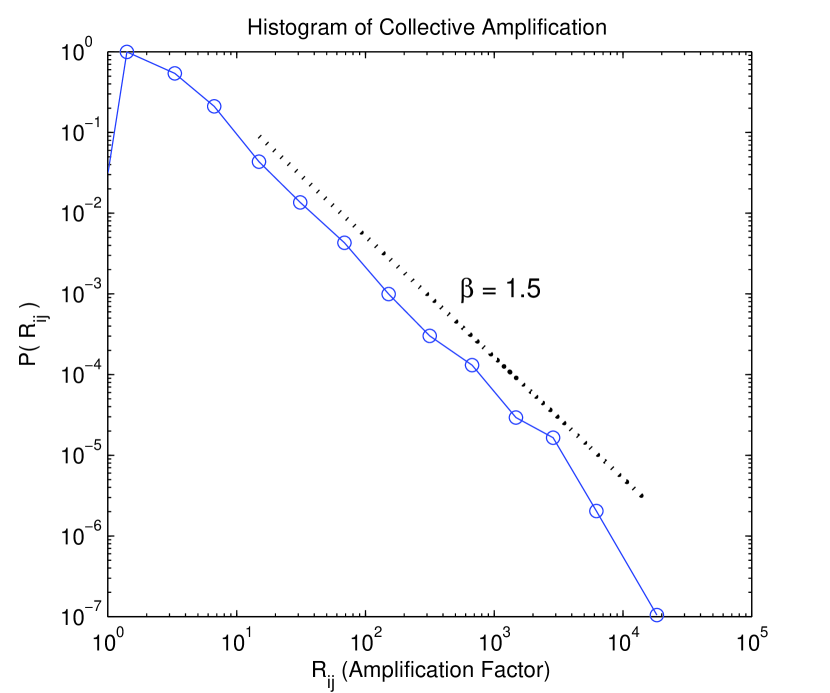
Figure 1: Histogram of amplification factors for spontaneous (thermal) noise of equilibrium dimer concentrations $D_{ij}$ in the PPI network of yeast. Collective effects lead to amplification relative to the isolated dimer null model. Large amplification, up to several orders of magnitude, is sometimes achieved.

Relative to the isolated case, collective amplification can lead to thermal noise that is orders of magnitude larger, as is evident from this histogram. The distribution has a power-law tail with an approximate exponent of $\beta\simeq 1.5$.

Collective amplification of thermal noise presents a worrisome theoretical possibility. Can amplification occur without limit? To address this question, it is fruitful to develop an alternative formalism in which the magnitude of fluctuations are calculated directly from the partition function. Using Eq. 2 it is straightforward to show, by a change of variables, that higher moments of $D_{ij}$ can be related to the lower moments evaluated at a reduced system size. In particular:

$$\langle D_{ij}(D_{ij}-1)\rangle=\langle D_{ij}\rangle\langle D_{ij}\rangle|_{C_{i}-1,C_{j}-1}$$

where the latter moment is evaluated in a system for which the copy number of proteins $i$ and $j$ ($C_{i}$ and $C_{j}$) are reduced by exactly one. It follows that the noise may be alternatively expressed as:

$$\eta=1+\langle D_{ij}\rangle|_{C_{i}-1,C_{j}-1}-\langle D_{ij}\rangle$$ (8)

The above expression for thermal noise hints at a connection to static perturbations of total concentration. This connection can be made even more explicit by expanding the 2nd term to first order in total concentration:

$$\eta\simeq 1-D_{ij}[(\Lambda^{-1})_{ii}+(\Lambda^{-1})_{jj}+2(\Lambda^{-1})_{ij}]$$ (9)

where the matrix:

$$\Lambda_{ij}=\frac{\partial C_{i}}{\partial\log F_{j}}=D_{ij}+C_{i}\delta_{ij}$$

characterizes the response of equilibrium concentrations $F_{m}$ to small static changes in total concentrations $C_{k}$ Sergei_NJP . It should be remarked that, despite the approximation used in Eq. 9, this approach is in good agreement with the FDT formalism first introduced. One notes that this expression for noise explicitly depends only on the total and dimer concentrations used to define the matrix $\Lambda$. This suggests the definition of a new isolated model (isol-C), consisting of an isolated $(ij)$ dimer formed by proteins with the same $C_{i}$, $C_{j}$ and $D_{ij}$. This is only possible through changes in the dissociation constant and free concentrations of constituent proteins $i$ and $j$. It is important to mention that this model is distinct from the isol-F benchmark defined earlier, in which each isolated dimer has the same equilibrium free and dimer concentrations (yet different $C_{i}$ and $C_{j}$) as the corresponding dimer in the network. For an isol-C dimer, the matrix $\Lambda$ is 2x2 and trivially invertible. The noise is given by:

$$\eta^{\mathrm{isol-C}}=\left(\frac{D_{ij}}{C_{i}-D_{ij}}+\frac{D_{ij}}{C_{j}-D_{ij}}+1\right)^{-1}$$ (10)

A comparison with the isol-F model reveals that a dimer in the isol-C model has an equilibrium free concentration $\tilde{F_{i}}=F_{i}+\sum_{k}{D_{ik}}$ and similarly for protein $j$. In other words, the contribution of neighboring dimers to the noise of dimer $(ij)$ has been included by absorbing them into an effective free concentration. Moreover, where the isol-F model completely ignores the effect of neighboring dimers, the isol-C model brings neighboring sources of noise one step closer to dimer $(ij)$. Consequently, the noise of a dimer in the isol-C model always exceeds the noise of a corresponding dimer in the real network. The real noise for a dimer in a network falls between the bounds of the two isolated dimer noise predictions. A summary of the lower- and upper-bound models and their noise is given in Fig. 2.

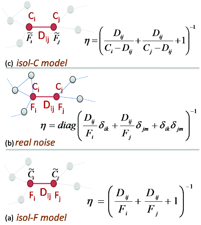
Figure 2: A comparison of the noise in a network dimer to two isolated dimer models defined in the text. (a) The isol-F model: Each dimer $(ij)$ is isolated and has the same protein free- ($F_{i}$, $F_{j}$) and dimer- concentrations ($D_{ij}$) as the corresponding dimer in the network. This model ignores the contribution of other dimers to the noise of dimer $(ij)$ (b) The noise of a dimer $(ij)$ in the network is given by the $(ij),(ij)$ diagonal element of the inverse of the matrix $\Gamma$ as described in the text. (c) The isol-C model: Each dimer $(ij)$ is isolated and has the same protein total- ($C_{i}$, $C_{j}$) and dimer- concentrations ($D_{ij}$) as the corresponding dimer in the network. The real noise is bound below and above by the isolated models $\eta^{\mathrm{isol-F}}<\eta<\eta^{\mathrm{isol-C}}$

The actual spontaneous fluctuations achieved are a result of real network topology and the distribution of total protein concentration. It is natural to ask how these fluctuations compare to their minimally and maximally achievable values. This suggests the coordinate transformation:

$$\eta\equiv(1-\zeta)\eta^{\mathrm{isol-F}}+\zeta\eta^{\mathrm{isol-C}}$$

A histogram of $\zeta$ for the PPI network of yeast is shown in Fig. 3. Of particular note is the large pileup against the upper limit of amplification. In real PPI networks, it would seem that collective effects lead to amplification quite close the maximally achievable limit.

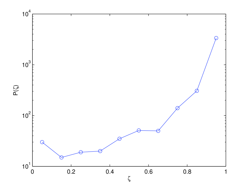
Figure 3: Histogram of the spontaneous noise coordinate $\zeta$ in the PPI network of yeast. The coordinate describes the position of noise amplitude relative to its lower ($\zeta=0$) and upper ($\zeta=1$) limits described in the text.

Now we turn our attention to the second type of noise driven by stochastic changes in protein copy number $C_{i}$. In the living cell, these fluctuations are typically much larger than the spontaneous fluctuations. Furthermore, the changes in $C_{i}$ occur at a relatively slow time scale (tens of minutes) so that the mass-action equilibrium respond to these changes. From the results of Sergei_NJP ; Sergei_PNAS it follows that, in general, the amplitude of driven fluctuations is given by:

$$\frac{\langle\delta D_{ij}^{2}\rangle}{D_{ij}^{2}}=\langle(\sum_{k}{(\Lambda^{-1})_{ik}}\delta C_{k}+\sum_{m}{(\Lambda^{-1})_{jm}\delta C_{m}})^{2}\rangle$$ (11)

The evaluation of the above expression requires the full matrix of cross-correlations $\langle\delta C_{k}\delta C_{m}\rangle$ which is currently experimentally unknown. For the simplest case $\langle\delta C_{k}\delta C_{m}\rangle\propto C_{k}^{2}\delta_{mk}$ of uncorrelated fluctuations (so-called intrinsic noise Bio_fluct ), the driven response becomes:

$$\left(\frac{\langle\delta D_{ij}^{2}\rangle}{D_{ij}^{2}}\right)_{\mathrm{int}}\propto\sum_{k}{[(\Lambda^{-1})_{ik}+(\Lambda^{-1})_{jk}]^{2}C_{k}^{2}}$$ (12)

In conclusion we study how the two types of noise studied above relate to simple predictors such as abundance and connectivity (number of connections a dimer has to the network). With high statistical significance, we find that the relative amplitude ($\sqrt{\langle\delta D_{ij}^{2}\rangle}/D_{ij}$) of both spontaneous and driven (intrinsic) noise is negatively correlated with dimer abundance $D_{ij}$ (Spearman coefficient of $r=-0.98$, $r=-0.64$, respectively). This result is generally expected for relative noise amplitudes due to the law of large numbers. Indeed, for independent fluctuations it is expected to decrease as $\sim 1/\sqrt{D_{ij}}$. This explains a particularly strong correlation in the case of spontaneous fluctuations. Furthermore, we found that relative amplitude of both spontaneous and driven (intrinsic) noise are positively correlated with connectivity ($r=0.46$, $r=0.34$). This is consistent with the overall scenario that we investigated above in which any type of noise propagates throughout the network and network connections (both direct and, to some extent, indirect) to noisy partners positively contribute to fluctuations of individual dimers.

Work at Brookhaven National Laboratory was carried out under Contract No. DE-AC02-98CH10886, Division of Material Science, U.S. Department of Energy.

References

- (1) M. B. Elowitz, A. J. Levine, E. D. Siggia, P. S. Swain, Science 297, 1183 (2002).
- (2) L. Laloux, P. Cizeau, J. Bouchaud, M. Potters, Phys. Rev. Lett. 83, 1467 (1999).
- (3) M. Takayusa, H. Takayusa, T. Sato, Physica A. 233, 824 (1996).
- (4) K. Nagel, M. Paczuski, Phys. Rev. E 51, 2909 (1995).
- (5) J. M. Pedraza, A. van Oudenaarden, Science 307, 1965 (2005).
- (6) E. Levine, T. Hwa, Proc. Natl. Acad. Sci. U.S.A. 104 9224 (2007).
- (7) S. Maslov, K. Sneppen and I. Ispolatov, New J. Phys. 9, 273 (2007).
- (8) S. Maslov and I. Ispolatov, Proc. Natl. Acad. Sci. U.S.A. 104, 34 (2007).
- (9) C. Stark, B. J. Breitkreutz, T. Reguly, L. Boucher, A. Breitkreutz andM. Tyers, Nucleic Acids Res., 34, D535 (2006).
- (10) S. Ghaemmaghami, W. K. Huh, K. Bower, R. W. Howson, A. Belle, N. Dephoure, E. K. O’Shea and J. S. Weissman, Nature, 425, 737 (2003).
- (11) I. Prigogine, Physica, 16, 134 (1950).
- (12) For brevity, assume the notation , . The matrix is symmetrized by the diagonal matrix and is diagonalized by a unitary transformation so that: . From these considerations and the convexity of it can be shown that , where and .