Scaled solar tracks and isochrones in a large region of the $Z$–$Y$ plane

Abstract

Context. In many astrophysical contexts, the helium content of stars may differ significantly from those usually assumed in evolutionary calculations.

Aims. In order to improve upon this situation, we have computed tracks and isochrones in the range of initial masses $0.15-20M_{\odot}$ for a grid of 39 chemical compositions with the metal content $Z$ between 0.0001 and 0.070 and helium content $Y$ between 0.23 and 0.46.

Methods. The Padova stellar evolution code has been implemented with updated physics. New synthetic TP-AGB models allow the extension of stellar models and isochrones until the end of the thermal pulses along the AGB. Software tools for the bidimensional interpolation (in $Y$ and $Z$) of the tracks have been tuned.

Results. This first paper presents tracks for low mass stars (from $0.15$ to $2.5M_{\odot}$) with scaled-solar abundances and the corresponding isochrones from very old ages down to about 1 Gyr.

Conclusions. Tracks and isochrones are made available in tabular form for the adopted grid of chemical compositions in the plane $Z-Y$. As soon as possible an interactive web interface will allow users to obtain isochrones of whatever chemical composition and also simulated stellar populations with different $Y(Z)$ helium-to-metal enrichment laws.

1 Introduction

Evolutionary tracks and isochrones are usually computed taking into account a fixed law of helium to metal enrichment $(\Delta Y/\Delta Z)$. In fact most of the available tracks follow a linear $Y(Z)$ relation of the form $Y=Y_{P}+(\Delta Y/\Delta Z)\,Z$ (e.g. Bertelli et al. 1994 with $Y_{\rm p}=0.23,\Delta Y/\Delta Z=2.5$; or Girardi et al. 2000, where $Y_{\rm p}=0.23,\Delta Y/\Delta Z=2.25$). Grids of stellar models in general used $\Delta Y/\Delta Z$ values higher than $\sim 2$ in order to fit both the primordial and the solar initial He content. On one side we recall that WMAP has provided a value of the primordial helium ($Y_{P}\sim 0.248$, Spergel et al. 2003, 2007), significantly higher than the value assumed in our previous stellar models. On the other side the determinations of the helium enrichment from nearby stars and K dwarfs or from Hyades binary systems show a large range of values for this ratio (Pagel & Portinari 1998, Jimenez et al. 2003, Casagrande et al. 2007, Lebreton et al. 2001). Therefore it is suitable to make available stellar models that can be used to simulate different enrichment laws.

Several new results suggest that the naive assumption that the helium enrichment law is universal, might not be correct. In fact there has been recently evidence of significant variations in the helium content (and perhaps of the age) in some globular clusters, that were traditionally considered as formed of a simple stellar population of uniform age and chemical composition. According to Piotto et al. (2005) and Villanova et al. (2007), only greatly enhanced helium can explain the color difference between the two main sequences in $\omega$ Cen. Piotto et al.(2007) attribute the triple main sequence in NGC 2808 to successive rounds of star formation, with different helium abundances. In NGC 2808 a helium enhanced population could explain the MS spread and the HB morphology ( Lee et al. 2005, D’Antona et al. 2005).

In general the main sequence morphology can allow to detect differences in helium content only when the helium content is really very large. Many globular clusters might have a population with enhanced helium (up to $Y=0.3-0.33$), but only a few have a small population with very high helium, such as suggested for NGC 2808. For NGC 6441 (Caloi & D’Antona 2007) a very large helium abundance is required to explain part of the horizontal branch population, that might be interpreted as due to self-enrichment and multiple star formation episodes in the early evolution of globular clusters. The helium self-enrichment in globular clusters has been discussed in several papers. Among them we recall Karakas et al. (2006) on the AGB self-pollution scenario, Maeder & Meynet (2006) on rotating low-metallicity massive stars, while Prantzos and Charbonnel (2006) discuss the drawbacks of both hypotheses.

This short summary of recent papers displays how much interest there is on the enriched helium content of some stellar populations. This is the reason why we started these new sets of evolutionary models allowing to simulate a large range of helium enrichment laws. There are a number of other groups producing extended databases of tracks and isochrones both for scaled solar and for $\alpha$-enhanced chemical compositions (Pietrinferni et al. 2004, 2006; Yi et al. 2001 and Demarque et al. 2004; VandenBerg et al. 2006), but their models usually take into account a fixed helium enrichment law. Unlike these authors, very recently Dotter et al. (2007) presented new stellar tracks and isochrones for three initial helium abundances in the range of mass between $0.1$ and $1.8\mbox{$M_{\odot}$}$ for scaled solar and $\alpha$-enhanced chemical compositions.

In this paper we present new stellar evolutionary tracks for different values of the initial He for each metal content. In fact homogeneous grids of stellar evolution models and isochrones in an extended region of the Z-Y plane and for a large range of masses are required for the interpretation of photometric and spectroscopic observations of resolved and unresolved stellar populations and for the investigation of the formation and evolution of galaxies.

Section 2 describes the input physics and the coverage of the Z-Y plane and Section 3 the new synthetic TP-AGB models. Section 4 presents the evolutionary tracks and relative electronic tables. Section 5 describes the derived isochrones and the interpolation scheme; Section 6 presents the comparison with other stellar models databases and Section 7 the concluding remarks.

2 Input physics and coverage of the $Z-Y$ plane

The stellar evolution code adopted in this work is basically the same as in Bressan et al. (1993), Fagotto et al. (1994a,b) and Girardi et al. (2000), but for updates in the opacities, in the rates of energy loss by plasma neutrinos (see Salasnich et al. 2000), and for the different way the nuclear network is integrated (Marigo et al. 2001). In the following we will describe the input physics, pointing out the differences with respect to Girardi et al. (2000).

2.1 Initial chemical composition

Table 1: Combinations of $Z$ and $Y$ of the computed tracks

Z	Y1	Y2	Y3	Y4	Y5	Y6
0.0001	0.23	0.26	0.30		0.40
0.0004	0.23	0.26	0.30		0.40
0.001	0.23	0.26	0.30		0.40
0.002	0.23	0.26	0.30		0.40
0.004	0.23	0.26	0.30		0.40
0.008	0.23	0.26	0.30	0.34	0.40
0.017	0.23	0.26	0.30	0.34	0.40
0.040		0.26	0.30	0.34	0.40	0.46
0.070			0.30	0.34	0.40	0.46

Stellar models are assumed to be chemically homogeneous when they settle on the zero age main sequence (ZAMS). Several grids of stellar models were computed from the ZAMS with initial mass from $0.15$ to $20M_{\odot}$. The first release of the new evolutionary models, presented in this paper, deals with very low and low mass stars up to $2.5M_{\odot}$. In general for each chemical composition the separation in mass is of $0.05M_{\odot}$ between $0.15$ and $0.6M_{\odot}$, of $0.1M_{\odot}$ between $0.6$ and $2.0M_{\odot}$. In addition evolutionary models at $2.20$ and $2.50M_{\odot}$ are computed in order to make available isochrones from the Hubble time down to 1 Gyr for each set of models. The initial chemical composition is in the range $0.0001\leq Z\leq 0.070$ for the metal content and for the helium content in the range $0.23\leq Y\leq 0.46$ as shown in Table 1. The helium content $Y=0.40$ was supplemented at very low metallicities as useful for simulations of significant helium enrichment in globular clusters.

For each value of $Z$, the fractions of different metals follow a scaled solar distribution, as compiled by Grevesse & Noels (1993) and adopted in the OPAL opacity tables. The ratio between abundances of different isotopes is according to Anders & Grevesse (1989).

2.2 Opacities

The radiative opacities for scaled solar mixtures are from the OPAL group (Iglesias & Rogers 1996) for temperatures higher than $\log T=4$, and the molecular opacities from Alexander & Ferguson (1994) for $\log T<4.0$ as in Salasnich et al. (2000). In the temperature interval $3.8<\log T<4.0$, a linear interpolation between the opacities derived from both sources is adopted. The agreement between both tables is excellent and the transition is very smooth in this temperature interval. For very high temperatures ($logT\geq 8.7$) opacities by Weiss et al. (1990) are used.

The conductive opacities of electron-degenerate matter are from Itoh et al. (1983), whereas in Girardi et al. (2000) conductive opacities were from Hubbard & Lampe (1969). A second difference with respect to Girardi et al. (2000) lies in the numerical tecnique used to interpolate within the grids of the opacity tables. In this paper we used the two-dimensional bi-rational cubic damped-spline algorythm (see Schlattl & Weiss 1998, Salasnich et al. 2000 and Weiss & Schlattl 2000).

2.3 Equation of state

The equation of state (EOS) for temperatures higher than $10^{7}$ K is that of a fully-ionized gas, including electron degeneracy in the way described by Kippenhahn et al. (1967). The effect of Coulomb interactions between the gas particles at high densities is taken into account as described in Girardi et al. (1996).

For temperatures lower than $10^{7}$ K, the detailed “MHD” EOS of Mihalas et al. (1990, and references therein) is adopted. The free-energy minimization technique used to derive thermodynamical quantities and derivatives for any input chemical composition, is described in detail by Hummer & Mihalas (1988), Däppen et al. (1988), and Mihalas et al. (1988). In our cases, we explicitly calculated EOS tables for all the $Z$ and $Y$ values of our tracks, using the Mihalas et al. (1990) code, as in Girardi et al. (2000). We recall that the MHD EOS is critical only for stellar models with masses lower than 0.7 $M_{\odot}$, during their main sequence evolution. In fact, only in dwarfs with masses lower than 0.7 $M_{\odot}$ the surface temperatures are low enough so that the formation of the H₂ molecule dramatically changes the adiabatic temperature gradient. Moreover, only for masses smaller than $\sim 0.4$ $M_{\odot}$ the envelopes become dense and cool enough so that the many non-ideal effects included in the MHD EOS (internal excitation of molecules, atoms, and ions; translational motions of partially degenerate electrons, and Coulomb interactions) become important.

2.4 Reaction rates and neutrino losses

The adopted network of nuclear reactions involves all the important reactions of the pp and CNO chains, and the most important alpha-capture reactions for elements as heavy as Mg (see Bressan et al. 1993 and Girardi et al. 2000).

The reaction rates are from the compilation of Caughlan & Fowler (1988), but for ${}^{17}{\rm O}({\rm p},\alpha)^{14}{\rm N}$ and ${}^{17}{\rm O}({\rm p},\gamma)^{18}{\rm F}$, for which we use the determinations by Landré et al. (1990). The uncertain ¹²C($\alpha,\gamma$)¹⁶O rate was set to 1.7 times the values given by Caughlan & Fowler (1988), as indicated by the study of Weaver & Woosley (1993) on the nucleosynthesis by massive stars.The adopted rate is consistent with the recent determination by Kunz et al. (2002) within the uncertainties. The electron screening factors for all reactions are those from Graboske et al. (1973). The abundances of the various elements are evaluated with the aid of a semi-implicit extrapolation scheme, as described in Marigo et al. (2001).

The energy losses by neutrinos are from Haft et al. (1994). Compared with the previous ones by Munakata et al. (1985) used in Girardi et al. (2000), neutrino cooling during the RGB is more efficient.

2.5 Convection

The extension of the convective regions is determined considering the presence of convective overshoot. The energy transport in the outer convection zone is described according to the mixing-length theory (MLT) of Böhm-Vitense (1958). The mixing length parameter $\alpha$ is calibrated by means of the solar model.

Overshoot The extension of the convective regions takes into account overshooting from the borders of both core and envelope convective zones. In the following we adopt the formulation by Bressan et al. (1981) in which the boundary of the convective core is set at the layer where the velocity (rather than the acceleration) of convective elements vanishes. Also this non-local treatment of convection requires a free parameter related to the mean free path $l$ of convective elements through $l=\Lambda_{c}H_{p}$, ($H_{p}$ being the pressure scale height). The choice of this parameter determines the extent of the overshooting across the border of the classical core (determined by the Schwarzschild criterion). Other authors fix the extent of the overshooting zone at the distance $d=\Lambda_{c}H_{p}$ from the border of the convective core (Schwarzschild criterion).

The $\Lambda_{c}$ parameter in Bressan et al.(1981) formalism is not equivalent to others found in literature. For instance, the overshooting extension determined by $\Lambda_{c}=0.5$ with the Padova formalism roughly corresponds to the $d=0.25H_{p}$ above the convective border, adopted by the Geneva group (Meynet et al. 1994 and references therein) to describe the same physical phenomenum. This also applies to the extent of overshooting in the case of models computed by Teramo group (Pietrinferni et al. 2004), in the Yale-Yonsei database (Yi et al. 2001 and Demarque et al. 2004), as they adopted the value 0.2 for the overshoot parameter above the border of the classical convective core. In Victoria-Regina stellar models by VandenBerg et al. (2006) a free parameter varying with mass is adopted to take into account overshoot in the context of Roxburgh’s equation for the maximum size of a central convective zone, so the comparison is not so straight. The non-equivalency of the parameter used to describe the extension of convective overshooting by different groups has been a recurrent source of misunderstanding in the literature.

We adopt the same prescription as in Girardi et al. (2000) for the parameter $\Lambda_{c}$ as a function of stellar mass. $\Lambda_{c}$ is set to zero for stellar masses $M\leq 1.0$ $M_{\odot}$, and for $M\geq 1.5\mbox{$M_{\odot}$}$, we adopt $\Lambda_{c}=0.5$, i.e. a moderate amount of overshoting. In the range $1.0<M<1.5\mbox{$M_{\odot}$}$, we adopt a gradual increase of the overshoot efficiency with mass, i.e. $\Lambda_{c}=M/\mbox{$M_{\odot}$}-1.0$. This because the calibration of the overshooting efficiency in this mass range is still very uncertain and from observations there are indications that this efficiency should be lower than in intermediate-mass stars.

In the stages of core helium burning (CHeB), the value $\Lambda_{c}=0.5$ is used for all stellar masses. This amount of overshooting significantly reduces the extent of the breathing pulses of convection found in the late phases of CHeB (see Chiosi et al. 1992).

Overshooting at the lower boundary of convective envelopes is also considered. The calibration of the solar model required an envelope overshooting not higher than 0.25 pressure scale height. This value of $\Lambda_{e}=0.25$ (see Alongi et al. 1991) was then adopted for the stars with $0.6\leq(M/\mbox{$M_{\odot}$})<2.0$, whereas $\Lambda_{e}=0$ was adopted for $M\la 0.6\mbox{$M_{\odot}$}$. For $M>2.5\mbox{$M_{\odot}$}$ a value of $\Lambda_{e}=0.7$ was assumed as in Bertelli et al. (1994) and Girardi et al. (2000). Finally, for masses between 2.0 and $2.5\mbox{$M_{\odot}$}$, $\Lambda_{e}$ was let to increase gradually from 0.25 to 0.7, but for the helium burning evolution, where it is always set to 0.7.

The adopted approach to overshooting perhaps does not represent the complex situation found in real stars. However it represents a pragmatic choice, supported by comparisons with observations. We recall that also the question of the overshooting efficiency in stars of different masses is still a matter of debate (see a recent discussion by Claret 2007, and by Deng and Xiong 2007).

Helium semiconvection As He-burning proceeds in the convective core of low mass stars during the early stages of the horizontal branch (HB), the size of the convective core increases. Once the central value of helium falls below $Y_{c}=0.7$, the temperature gradient reaches a local minimum, so that continued overshoot is no longer able to restore the neutrality condition at the border of the core. The core splits into an inner convective core and an outer convective shell. As further helium is captured by the convective shell, this latter tends to become stable, leaving behind a region of varying composition in condition of neutrality. This zone is called semiconvective. Shortly, starting from the center and going outwards, the matter in the radiatively stable region above the formal convective core is mixed layer by layer until the neutrality condition is achieved. This picture holds during most of the central He-burning phase.

The extension of the semiconvective region varies with the stellar mass, being important in the low- and intermediate-mass stars up to about $5M_{\odot}$, and negligible in more massive stars. We followed the scheme by Castellani et al. (1985), as described in Bressan et al. (1993).

Breathing convection As central helium gets as low as $Y_{c}\simeq 0.1$, the enrichment of fresh helium caused by semiconvective mixing enhances the rate of energy produced by the $3\alpha$ reactions in such a way that the radiative gradient at the convective edge is increased. A very rapid enlargement followed by an equally rapid decrease of the fully convective core takes place (pulse of convection). Several pulses may occur before the complete exhaustion of the central helium content. This convective instability was called breathing convection by Castellani et al. (1985). While semiconvection is a true theoretical prediction, the breathing pulses are most likely an artifact of the idealized algorithm used to describe mixing (see Bressan et al. 1993 and references therein). In our code breathing pulses are suppressed by imposing that the core cannot be enriched in helium by mixing with the outer layers more than a fixed fraction F of the amount burnt by nuclear reactions. In this way a time dependence of convection is implicitely taken into account.

2.6 Calibration of the solar model

Recent models of the Sun’s evolution and interior show that currently observed photospheric abundances (relative to hydrogen) must be lower than those of the proto-Sun because helium and other heavy elements have settled toward the Sun’s interior since the time of its formation about 4.6 Gyr ago. The recent update of the solar chemical composition (Asplund et al 2005, 2006 and Montalban et al. 2006) has led to a decrease in the CNO and Ne abundances of the order of $30\%$. Their new solar chemical composition corresponds to the values: $X=0.7393,Y=0.2485,Z=0.0122$ with $Z/X=0.0165$. The corresponding decrease in opacity increases dramatically the discrepancies between the sound-speed derived from helioseismology and the new standard solar model (SSM). Combinations of increases in opacity and diffusion rates are able to restore part of the sound-speed profile agreement, but the required changes are larger than the uncertainties accepted for the opacity and the diffusion uncertainties. Antia and Basu (2006) investigated the possibility of determining the solar heavy-element abundances from helioseismic data, used the dimensionless sound-speed derivative in the solar convection zone and gave a mean value of $Z=0.0172\pm 0.002$.

Bahcall et al.(2006) used Monte Carlo simulations to determine the uncertainties in solar model predictions of parameters measured by helioseismology (depth of the convective zone, the surface helium abundance, the profiles of the sound speed and density versus radius) and provided determinations of the correlation coefficients of the predicted solar model neutrino fluxes. They incorporated both the Asplund et al. recently determined heavy element abundances and the higher abundances by Grevesse & Sauval (1998). Their Table 7 points out that the derived characteristic solar model quantities are significantly different for the two cases.

According to VandenBerg et al. (2007) the new Asplund et al. metallicity for the Sun presents some difficulties for fits of solar abundance models to the M67 CMD, in that they do not predict a gap near the turnoff, which however is observed. If the Asplund et al. solar abundances are correct, only those low-Z solar models that treat diffusion may be able to reproduce the M67 CMD.

Owing to the many uncertainties, we adopted for the Sun the initial metallicity of $Z=0.017$, according to Grevesse & Sauval (1998). Our choice is a compromise between the previous solar metal content, Z=0.019 or 0.020, usually considered for evolutionary models and the significantly lower value supported by Asplund et al. (2005, 2006).

The usual procedure for the calibration of the solar model is of computing a number of models while varying the MLT parameter $\alpha$ and the initial helium content $Y_{0}$ until the observed solar radius and luminosity are reproduced within a predetermined range. Several 1 $M_{\odot}$ models, for different values of the mixing-length parameter $\alpha$ and helium content $Y_{\odot}$, are let to evolve up to the age of 4.6 Gyr. From this series of models, we are able to single out the pair of $[\alpha,Y_{\odot}]$ which allows for a simultaneous match of the present-day solar radius and luminosity, $R_{\odot}$ and $L_{\odot}$. An additional constraint for the solar model comes from the helioseismological determination of the depth of the outer solar convective zone ($R_{c}$ of the order of $0.710-0.716$ $R_{\odot}$) and from the surface helium value. The envelope overshooting parameter was adopted as $\Lambda_{e}=0.25$, which allows a reasonable reproduction of the observed value of $R_{c}$ (depth of the solar convective envelope).

Our final solar model reproduces well the solar $R_{\odot}$, $L_{\odot}$, and $R_{\rm c}$ values. The differences with respect to observed values are smaller than 0.2 % for $R_{\odot}$ and $L_{\odot}$, and $\sim 1$ % for $R_{\rm c}$. From this model with initial $Z_{\odot}=0.017$ we derive the value of initial helium $Y_{\odot}=0.260$ and $\alpha=1.68$ (this value of the mixing-length parameter was used in all our stellar models as described previously).

2.7 Mass loss on the RGB

Our evolutionary models were computed at constant mass for all stages previous to the TP-AGB. However, mass loss by stellar wind during the RGB of low-mass stars is taken into account at the stage of isochrone construction. We use the empirical formulation by Reimers (1975), with the mass loss rate expressed in function of the free parameter $\eta$, by default assumed as 0.35 in our models (see Renzini & Fusi-Pecci 1988). The procedure is basically the following: we integrate the mass loss rate along the RGB of every single track, in order to estimate the actual mass of the correspondent model of ZAHB. See Bertelli et al. (1994) for a more detailed description.

This approximation is a good one since the mass loss does not affect significantly the internal structure of models along the luminous part of the RGB.

3 New synthetic TP-AGB models

An important update of the database of evolutionary tracks is the extension of stellar models and isochrones until the end of the thermal pulses along the Asymptotic Giant Branch, particularly relevant for stellar population analyses in the near-infrared, where the contribution of AGB stars to the integrated photometric properties is significant.

The new synthetic TP-AGB models have been computed with the aid of a synthetic code that has been recently revised and updated in many aspects as described in the paper by Marigo & Girardi (2007), to which the reader should refer for all details. It should be emphasized that the synthetic TP-AGB model in use does not provide a mere analytic description of this phase, since one key ingredient is a complete static envelope model which is numerically integrated from the photosphere down to the core. The basic structure of the envelope model is the same as the one used in the Padova stellar evolution code.

The major improvements are briefly recalled below.

• Luminosity. Thanks to high-accuracy formalisms (Wagenhuber & Groenewegen 1998; Izzard et al. 2004) we follow the complex behaviour of the luminosity due to the flash-driven variations and the over-luminosity effect caused by hot-bottom burning (HBB).
  

• Effective temperature. One fundamental improvement is the adoption of molecular opacities coupled to the actual surface C/O ratio (Marigo 2002), in place of tables valid for scaled solar chemical compositions (e.g. Alexander & Ferguson 1994). The most significant effect is the drop of the effective temperature as soon as C/O increases above unity as a consequence of the third dredge-up, in agreement with observations of carbon stars.
  

• The third dredge-up. We use a more realistic description of the process as a function of stellar mass and metallicity, with the aid of available analytic relations of the characteristic parameters, i.e. minimum core mass $M_{\rm c}^{\rm min}(M,Z)$ and efficiency $\lambda(M,Z)$, as derived from full AGB calculations (Karakas et al. 2002).
  

• Pulsation properties. A first attempt is made to account for the switching between different pulsation modes along the AGB evolution. Basing on available pulsation models for long period variables (LPV; Fox & Wood 1982, Ostlie & Cox 1986) we derive a criterion on the luminosity to predict the transition from the first overtone mode to the fundamental one (and viceversa).
  

• Mass-loss rates. These are evaluated with the aid of different formalisms, based on dynamical atmosphere models for LPVs, depending not only on stellar mass, luminosity, effective temperature, and pulsation period, but also on the chemical type, namely: Bowen & Willson (1991) for C/O $<1$, and Wachter et al. (2002) for C/O $>1$.

It should be also emphasized that in Marigo & Girardi (2007) the free parameters of the synthetic TP-AGB model – i.e. the minimum core mass $M_{\rm c}^{\rm min}$ and efficiency $\lambda$ – were calibrated as a function of stellar mass and metallicity, on the base of two basic observables derived for both Magellanic Clouds (MC), namely: i) the counts of AGB stars (for both M- and C-types) in stellar clusters and ii) the carbon star luminosity functions in galaxy fields. As illustrated by Girardi & Marigo (2007), the former observable quantifies the TP-AGB lifetimes for both the oxygen- and carbon-rich phase as a function of stellar mass and metallicity and it helps to determine $M_{\rm c}^{\rm min}$. The latter observable provides complementary constraints to both $M_{\rm c}^{\rm min}$ and $\lambda$ and their dependence on stellar mass and metallicity.

The calibration carried out by Marigo & Girardi (2007) has been mainly motivated by the aim of assuring that for that set of TP-AGB tracks, the predicted luminosities and lifetimes, hence the nuclear fuel of this phase, are correctly evaluated.

The same dredge-up parameters as derived by Marigo & Girardi (2007) have been adopted for computing the present sets of TP-AGB tracks, despite of the fact that they are chacterized by different initial conditions at the first thermal pulse (e.g. $M_{\rm c},\,T_{\rm eff},\,L$), and different chemical compositions of the envelope. This fact implies that the new sets of TP-AGB tracks are, to a certain extent, un-calibrated since no attempt was made to have our basic set of observables reproduced.

However, the choice to keep the same model paramemeters as derived from the MG07 calibration is still a meaningful option since the present TP-AGB models a) include already several important improvements in the treatment of the TP-AGB phase, as recalled at the beginning of this section; b) they constitute the reference grid from which we will start the new calibration procedure. The preliminary step will be to adopt a reasonable enrichment law, i.e. $Y_{P}$ (zero point) and the $\Delta Y/\Delta Z$ (slope) so as to limit the calibration of the free parameters to TP-AGB models belonging to a particular subset of initial ($Y,\,Z$) combinations. This work is being undertaken.

a)

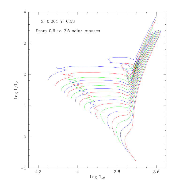
b)

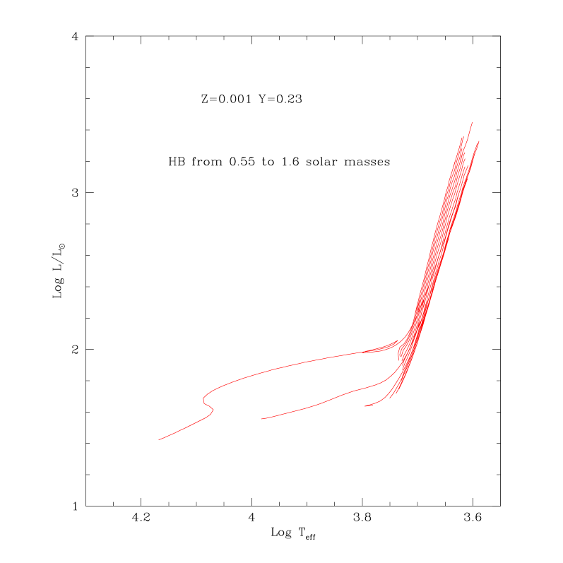
c)

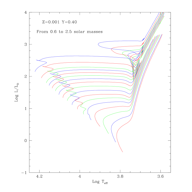
d)

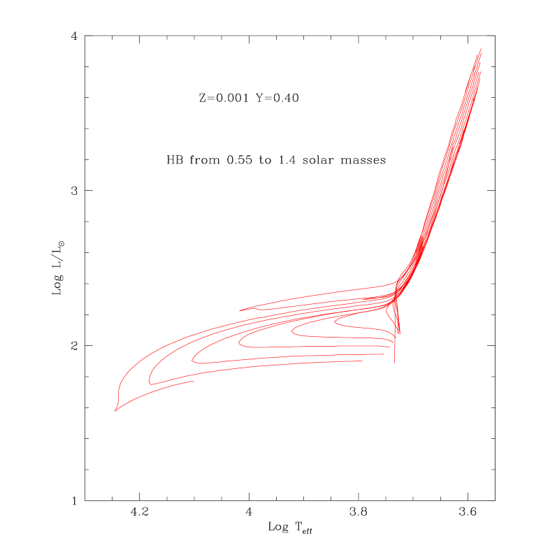
Figure 1: Evolutionary tracks in the HR diagram, for the composition $[Z=0.001,Y=0.23]$. For tracks of low-mass stars up to the RGB-tip and intermediate-mass ones ($M\leq 2.5M_{\odot}$) up to the bTP-AGB (panel a), and from the ZAHB up to the bTP-AGB (panel b). In panels c) and d) tracks are displayed for $[Z=0.001,Y=0.40]$

a)

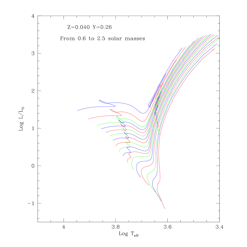
b)

c)

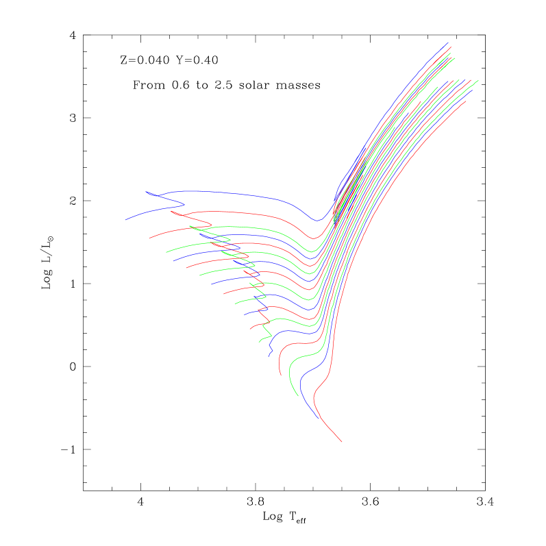
d)

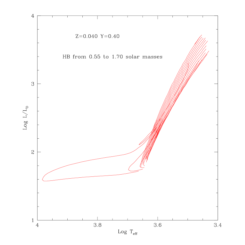
Figure 2: Evolutionary tracks in the HR diagram, for the composition $[Z=0.040,Y=0.26]$. For tracks of low-mass stars up to the RGB-tip and intermediate-mass ones up to the bTP-AGB (panel a), and from the ZAHB up to the bTP-AGB (panels b). In panels c) and d) tracks are displayed for $[Z=0.040,Y=0.40]$

a)

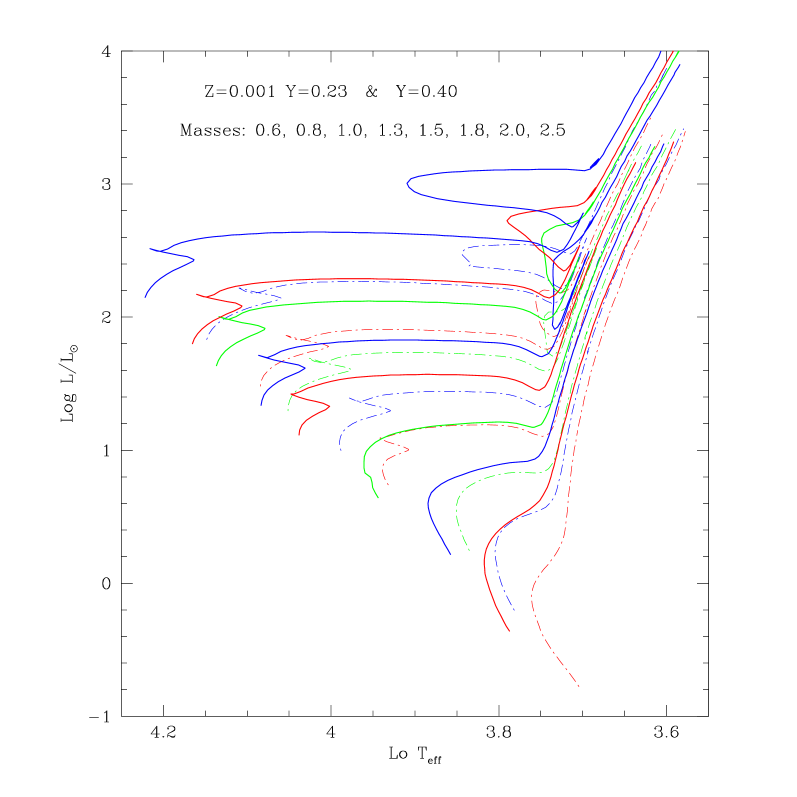
b)

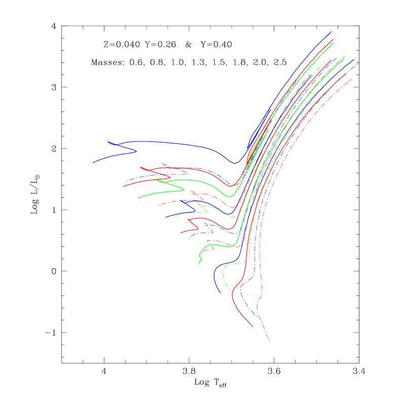
Figure 3: Evolutionary tracks in the HR diagram, for the composition $[Z=0.001,Y=0.23$ (dot-dashed line) and $Y=0.40$ (solid line)] in panel a). In panel b) tracks are displayed for $[Z=0.040,Y=0.26$ (dot-dashed line) and $Y=0.40$ (solid line)].

4 Stellar tracks

4.1 Evolutionary stages and mass ranges

Our models are evolved from the ZAMS and the evolution through the whole H- and He-burning phases is followed in detail. The tracks are stopped at the beginning of the TP-AGB phase (bTP-AGB) in intermediate- and low-mass stars. In the case of stellar masses lower than 0.6 $M_{\odot}$, the main sequence evolution takes place on time scales much longer than a Hubble time. For them, we stopped the computations at an age of about 20 Gyr.

In low-mass stars with $0.6M_{\odot}\leq M\leq M_{Hef}$ the evolution is interrupted at the stage of He-flash in the electron degenerate hydrogen-exhausted core. The evolution is then re-started from a ZAHB model with the same core mass and surface chemical composition as the last RGB model. For the core we compute the total energy difference between the last RGB model and the ZAHB configuration and assume it has been provided by helium burning during the helium flash phase. In this way a certain amount of the helium in the core is converted into carbon (about 3 percent in mass, depending on the stellar mass and initial composition), and the initial ZAHB model takes into account the approximate amount of nuclear fuel necessary to lift the core degeneracy during the He-flash. The evolution is then followed along the HB up to the bTP-AGB phase. We point out that this procedure is more detailed than the one adopted in Girardi et al. (2000), where the fraction of He core burnt during the He-flash was assumed to be constant and equal to 5%.

In intermediate-mass stars, the evolution goes from the ZAMS up to either the beginning of the TP-AGB phase, or to the carbon ignition in our more massive models (in this paper we consider masses up to $2.5\leavevmode\nobreak\ \mbox{$M_{\odot}$}$).

Table 2 gives the values of the transition mass $M\mbox{${}_{\rm Hef}$}$  as derived from the present tracks. $M\mbox{${}_{\rm Hef}$}$ is the maximum mass for a star to develop an electron-degenerate core after the main sequence, and sets the limit between low- and intermediate-mass stars (see e.g. Chiosi et al. 1992). Given the low mass separation between the tracks we computed, the $M\mbox{${}_{\rm Hef}$}$ values here presented are uncertain by about 0.05 $M_{\odot}$,

Table 2: The transition mass $M\mbox{${}_{\rm Hef}$}$

	$Y$
$Z$	0.23	0.26	0.30	0.34	0.40	0.46
0.0001	1.70	1.70	1.60		1.40
0.0004	1.70	1.60	1.50		1.40
0.001	1.60	1.60	1.50		1.40
0.002	1.70	1.60	1.50		1.40
0.004	1.80	1.75	1.60		1.40
0.008	1.90	1.85	1.75	1.60	1.40
0.017	2.10	2.00	1.90	1.70	1.60
0.040		2.20	2.05	1.90	1.70	1.40
0.070			2.05	1.80	1.60	1.40

4.2 Tracks in the HR diagram

The complete set of tracks for very low-mass stars ($M<0.6$ $M_{\odot}$) are computed starting at a stage identified with the ZAMS, and end at the age of 20 Gyr. The ZAMS model is defined to be the stage of minimum $T\mbox{${}_{\rm eff}$}$ along the computed track; it follows a stage of much faster evolution in which the pp-cycle is out of equilibrium, and in which gravitation may provide a non negligible fraction of the radiated energy. It is well known that these stars evolve very little during the Hubble time.

We display in Figures 1 and 2 only some examples of the sets of the computed evolutionary tracks (i.e. $[Z=0.001$ for $Y=0.23$ and $Y=0.40]$ and $[Z=0.040$ for $Y=0.26$ and $Y=0.40]$). In these figures, panel a) and c) present the tracks for masses between 0.6 and 2.5 $M_{\odot}$ from the ZAMS up to the RGB-tip, or to the bTP-AGB, while in panel b) and d) the low-mass tracks from the ZAHB up to the bTP-AGB phase are plotted from $0.55M_{\odot}$ to $M_{Hef}$. Figure 3 is aimed to illustrate the range of temperatures and luminosities involved for the boundary values of helium content at given metallicity in the theoretical HR diagram. The reader can notice, for instance, that at low metallicity and high helium (Z=0.001, Y=0.040) loops begin to be present during the core He burning phase, while they are practically missing in the $Z=0.040$ ones for masses about $2.5M_{\odot}$.

4.3 Description of the tables

The data tables for the present evolutionary tracks are available only in electronic format. A website with the complete data-base (including additional data and future extensions) will be mantained at http://stev.oapd.inaf.it/YZVAR.

For each evolutionary track, the corresponding data file presents 23 columns with the following information:

1. n: row number;

2. age/yr: stellar age in yr;

3. logL: logarithm of surface luminosity (in solar units), $\log(L/L_{\odot})$;

4. logTef: logarithm of effective temperature (in K), $\log T\mbox{${}_{\rm eff}$}$;

5. grav: logarithm of surface gravity ( in cgs units);

6. logTc: logarithm of central temperature (in K);

7. logrho: logarithm of central density (in cgs units);

8. Xc: mass fraction of hydrogen in the stellar centre;

9. Yc: mass fraction of helium in the stellar centre;

10. Xc_C: mass fraction of carbon in the stellar centre;

11. Xc_O: mass fraction of oxygen in the stellar centre;

12. Q_conv: fractionary mass of the convective core;

13. Q_disc: fractionary mass of the first mesh point where the chemical composition differs from the surface value;

14. L_H/L: fraction of the total luminosity provided by H-burning reactions;

15. Q1_H: fractionary mass of the inner border of the H-rich region;

16. Q2_H: fractionary mass of the outer border of the H-burning region;

17. L_He/L: fraction of the total luminosity provided by He-burning reactions;

18. Q1_He: fractionary mass of the inner border of the He-burning region;

19. Q2_He: fractionary mass of the outer border of the He-burning region;

20. L_C/L: fraction of the total luminosity provided by C-burning reactions;

21. L_nu/L: fraction of the total luminosity lost by neutrinos;

22. Q_Tmax: fractionary mass of the point with the highest temperature inside the star;

23. stage: label indicating particular evolutionary stages.

A number of evolutionary stages are indicated along the tracks (column 23). They correspond either to: the beginning/end of main evolutionary stages, local maxima and minima of $L$ and $T\mbox{${}_{\rm eff}$}$, and main changes of slope in the HR diagram. These particular stages were, in general, detected by an authomated algorithm. They can be useful for the derivation of physical quantities (as e.g. lifetimes) as a function of mass and metallicity, and are actually used as equivalent evolutionary points in our isochrone-making routines.

For TP-AGB tracks during the quiescent stages of evolution preceding He-shell flashes, our tables provide:

1. n: row number;

2. age/yr: stellar age in yr;

3. logL: logarithm of surface luminosity (in solar units), $\log(L/L_{\odot})$;

4. logTef: logarithm of effective temperature (in K), $\log T\mbox{${}_{\rm eff}$}$;

5. Mact: the current mass (in solar units);

6. Mcore: the mass of the H-exhausted core (in solar units);

7. C/O: the surface C/O ratio.

4.4 Changes in surface chemical composition

The surface chemical composition of the stellar models changes on two well-defined dredge-up events. The first one occurs at the first ascent of the RGB for all stellar models (except for the very-low mass ones which are not evolved out of the main sequence). The second dredge-up is found after the core He-exhaustion, being remarkable only in models with $M\ga 3.5$ $M_{\odot}$. We provide tables with the surface chemical composition of H, ³He, ⁴He, and main CNO isotopes, before and after the first dredge-up, as in this paper we present models from $0.15$ up to $2.5M_{\odot}$. Table 3 shows, as an example, the surface abundances for the chemical composition Z=0.008 and Y=0.26.

Table 3: Surface chemical composition (by mass fraction) of $[Z=0.008,Y=0.26]$ models.

$M/\mbox{$M_{\odot}$}$	H	3He	4He	12C	13C	14N	15N	16O	17O	18O
Initial:
all	0.732	2.78$\>10^{-5}$	0.260	1.37$\>10^{-3}$	1.65$\>10^{-5}$	4.24$\>10^{-4}$	1.67$\>10^{-6}$	3.85$\>10^{-3}$	1.56$\>10^{-6}$	8.68$\>10^{-6}$
After the first dredge-up:
0.55	0.719	2.65$\>10^{-3}$	0.270	1.27$\>10^{-3}$	3.99$\>10^{-5}$	5.10$\>10^{-4}$	1.34$\>10^{-6}$	3.85$\>10^{-3}$	1.57$\>10^{-6}$	8.55$\>10^{-6}$
0.60	0.719	2.94$\>10^{-3}$	0.270	1.26$\>10^{-3}$	2.91$\>10^{-5}$	5.44$\>10^{-4}$	1.41$\>10^{-6}$	3.85$\>10^{-3}$	1.66$\>10^{-6}$	8.31$\>10^{-6}$
0.65	0.715	2.34$\>10^{-3}$	0.274	1.30$\>10^{-3}$	3.49$\>10^{-5}$	4.91$\>10^{-4}$	1.38$\>10^{-6}$	3.85$\>10^{-3}$	1.59$\>10^{-6}$	8.52$\>10^{-6}$
0.70	0.715	2.40$\>10^{-3}$	0.274	1.29$\>10^{-3}$	3.27$\>10^{-5}$	4.96$\>10^{-4}$	1.40$\>10^{-6}$	3.85$\>10^{-3}$	1.63$\>10^{-6}$	8.45$\>10^{-6}$
0.80	0.712	1.83$\>10^{-3}$	0.278	1.26$\>10^{-3}$	4.48$\>10^{-5}$	5.26$\>10^{-4}$	1.31$\>10^{-6}$	3.85$\>10^{-3}$	1.61$\>10^{-6}$	8.46$\>10^{-6}$
0.90	0.709	1.43$\>10^{-3}$	0.281	1.18$\>10^{-3}$	4.52$\>10^{-5}$	6.13$\>10^{-4}$	1.22$\>10^{-6}$	3.85$\>10^{-3}$	1.68$\>10^{-6}$	8.24$\>10^{-6}$
1.00	0.708	1.17$\>10^{-3}$	0.283	1.12$\>10^{-3}$	4.55$\>10^{-5}$	6.86$\>10^{-4}$	1.15$\>10^{-6}$	3.85$\>10^{-3}$	1.73$\>10^{-6}$	7.92$\>10^{-6}$
1.10	0.708	9.56$\>10^{-4}$	0.283	1.07$\>10^{-3}$	4.54$\>10^{-5}$	7.40$\>10^{-4}$	1.09$\>10^{-6}$	3.85$\>10^{-3}$	1.84$\>10^{-6}$	7.64$\>10^{-6}$
1.20	0.710	8.20$\>10^{-4}$	0.281	1.03$\>10^{-3}$	4.56$\>10^{-5}$	7.90$\>10^{-4}$	1.03$\>10^{-6}$	3.85$\>10^{-3}$	2.25$\>10^{-6}$	7.40$\>10^{-6}$
1.30	0.711	7.25$\>10^{-4}$	0.280	9.92$\>10^{-4}$	4.60$\>10^{-5}$	8.36$\>10^{-4}$	9.80$\>10^{-7}$	3.85$\>10^{-3}$	2.46$\>10^{-6}$	7.19$\>10^{-6}$
1.40	0.712	6.41$\>10^{-4}$	0.279	9.50$\>10^{-4}$	4.59$\>10^{-5}$	8.85$\>10^{-4}$	9.25$\>10^{-7}$	3.85$\>10^{-3}$	3.14$\>10^{-6}$	6.94$\>10^{-6}$
1.50	0.713	5.71$\>10^{-4}$	0.279	9.25$\>10^{-4}$	4.56$\>10^{-5}$	9.19$\>10^{-4}$	9.00$\>10^{-7}$	3.84$\>10^{-3}$	1.12$\>10^{-5}$	6.78$\>10^{-6}$
1.60	0.712	5.22$\>10^{-4}$	0.280	9.05$\>10^{-4}$	4.54$\>10^{-5}$	9.68$\>10^{-4}$	8.81$\>10^{-7}$	3.80$\>10^{-3}$	1.50$\>10^{-5}$	6.68$\>10^{-6}$
1.70	0.711	4.46$\>10^{-4}$	0.281	8.92$\>10^{-4}$	4.52$\>10^{-5}$	1.03$\>10^{-3}$	8.63$\>10^{-7}$	3.75$\>10^{-3}$	1.83$\>10^{-5}$	6.57$\>10^{-6}$
1.80	0.709	3.99$\>10^{-4}$	0.283	8.81$\>10^{-4}$	4.51$\>10^{-5}$	1.09$\>10^{-3}$	8.50$\>10^{-7}$	3.70$\>10^{-3}$	1.59$\>10^{-5}$	6.50$\>10^{-6}$
1.85	0.707	3.73$\>10^{-4}$	0.284	8.77$\>10^{-4}$	4.44$\>10^{-5}$	1.13$\>10^{-3}$	8.49$\>10^{-7}$	3.66$\>10^{-3}$	1.64$\>10^{-5}$	6.46$\>10^{-6}$
1.90	0.706	3.54$\>10^{-4}$	0.285	8.77$\>10^{-4}$	4.43$\>10^{-5}$	1.14$\>10^{-3}$	8.46$\>10^{-7}$	3.64$\>10^{-3}$	1.81$\>10^{-5}$	6.44$\>10^{-6}$
2.00	0.706	3.19$\>10^{-4}$	0.285	8.71$\>10^{-4}$	4.42$\>10^{-5}$	1.17$\>10^{-3}$	8.43$\>10^{-7}$	3.62$\>10^{-3}$	1.47$\>10^{-5}$	6.40$\>10^{-6}$
2.20	0.702	2.58$\>10^{-4}$	0.289	8.55$\>10^{-4}$	4.44$\>10^{-5}$	1.26$\>10^{-3}$	8.22$\>10^{-7}$	3.54$\>10^{-3}$	1.37$\>10^{-5}$	6.31$\>10^{-6}$
2.50	0.699	2.00$\>10^{-4}$	0.292	8.42$\>10^{-4}$	4.43$\>10^{-5}$	1.33$\>10^{-3}$	8.07$\>10^{-7}$	3.49$\>10^{-3}$	1.06$\>10^{-5}$	6.21$\>10^{-6}$

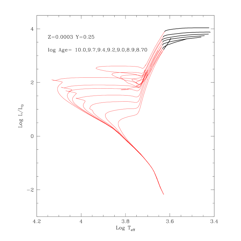
Figure 4: Isochrones for a chemical composition intermediate among those of the computed tracks (Z=0.0003,Y=0.25) at Log Age= 10, 9.7, 9.4, 9.0, 8.9 and 8.7 years.The new synthetic TP-AGB models allow the extension of the isochrones (red) until the end of the thermal pulses along the AGB (black).

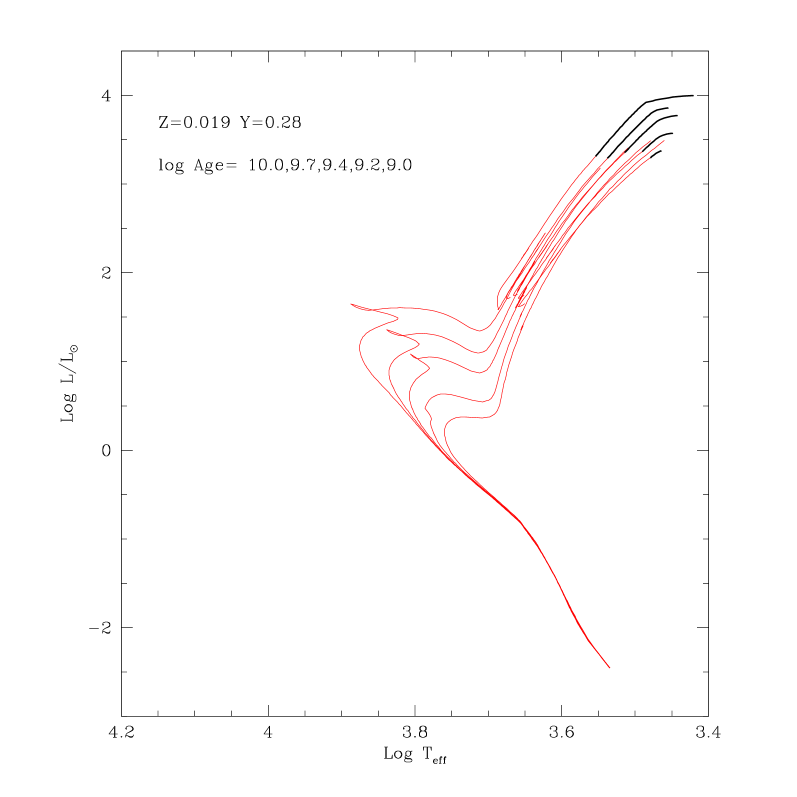
Figure 5: Isochrones for the chemical composition Z=0.019 and Y=0.28, intermediate among those of the computed tracks at Log Age= 10, 9.7, 9.4, 9.0 years. The same as Figure 4 for the AGB.

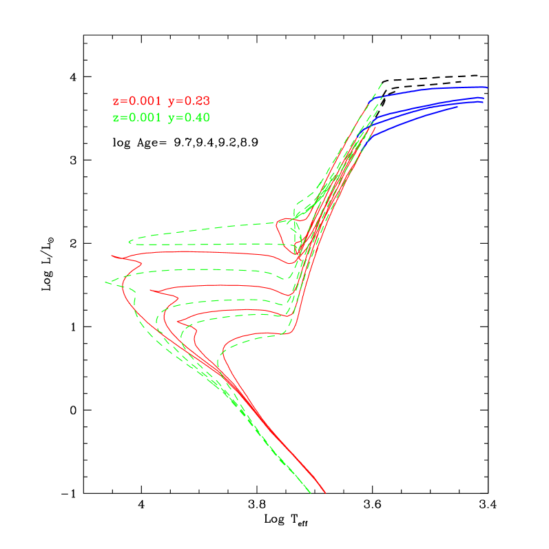
Figure 6: Comparison of isochrones for the same Z=0.001 and different helium content. Solid lines correspond to Y=0.23, dashed ones to Y=0.40. Also in this case the isochrones are extended until the end of the thermal pulses along the AGB.

5 Isochrones

From the tracks presented in this paper, we have constructed isochrones updating and improving the algorithm of “equivalent evolutionary points” used in Bertelli et al. (1994) and Girardi et al. (2000). The initial point of each isochrone is the 0.15 $M_{\odot}$ model in the lower main sequence. The terminal stage of the isochrones is the tip of the TP-AGB for the evolutionary tracks presented in this first paper (up to 2.5 $M_{\odot}$). We recall that usually there are small differences in the logarithm of the effective temperature between the last model of the track after the central He-exhaustion and the starting point of the synthetic TP-AGB model of the correspondent mass. Constructing the isochrones we removed these small discontinuities with a suitable shift. The differences arise as the Alexander & Ferguson (1994) low-temperature opacity tables, used for the evolutionary models, are replaced by those provided by Marigo’s (2002) algorithm from the beginning to the end of the TP-AGB phase.

In Figures 4 and 5 isochrones are shown for the chemical composition (Z=0.0003,Y=0.25) and (Z=0.019,Y=0.28) intermediate among those of the evolutionary tracks. The interpolation method to obtain the isochrone for a specific composition intermediate between the values of the computed tracks is described in the following subsection. In Figures 4, 5 and 6 the plotted isochrones are extended until the end of the TP-AGB phase and a different line color points out this phase in the theoretical HR diagram. The flattening of the AGB phase of the isochrones marks the transition from M stars to Carbon stars ($C/O>1$).

An increase of the helium content at the same metallicity in stellar models causes a decrease in the mean opacity and an increase in the mean molecular weight of the envelope (Vemury and Stothers, 1978), and in turn higher luminosities, hotter effective temperatures and shorter hydrogen and helium lifetimes of stellar models. Apparently in contradiction with the previous statement of higher luminosity for helium increase in evolutionary tracks, the evolved portion of the isochrones with lower helium are more luminous, as shown in figure 6 where we plot isochrones with Z=0.001 for Y=0.23 and Y=0.40. This effect is related to the interplay between the increase in luminosity and the decrease in lifetime of stellar models with higher helium content (at the same mass and metallicity).

5.1 Interpolation scheme

The program ZVAR, already used in many papers (for instance in Ng et al. 1995, Aparicio et al. 1996, Bertelli & Nasi 2001, Bertelli et al. 2003) has been extended to obtain isochrones and to simulate stellar populations in a large region of the $Z-Y$ plane (now its name is YZVAR). For each of a few discrete values of the metallicity of former evolutionary tracks there was only one value of the helium content, derived from the primordial helium with a fixed enrichment law. In the present case we deal with 39 sets of stellar tracks in the plane $Z-Y$ and we aim at obtaining isochrones for whatever $Z-Y$ combination and stellar populations with the required Y(Z) enrichment laws. This problem requires a double interpolation in Y and Z. We try to describe our method with the help of Figure 7. In this figure the corners of the box represent 4 different chemical compositions in a generic mesh of the grid, i.e. $(Y_{1},Z_{1})$, $(Y_{2},Z_{1})$, $(Y_{2},Z_{2})$, $(Y_{1},Z_{2})$.

Figure 7: Interpolation scheme inside the range [Z1,Z2] and [Y1,Y2].

The vertical lines departing from the corners represent the sequences of increasing mass of the tracks computed for the corresponding values of $(Y,Z)$. Along each of these lines the big points represent the separation masses between tracks with a different number of characteristic points ( a different number of equivalent evolutionary phases), indicated as $M_{Y_{1}Z_{1}{\rm sep}}^{i}$, $M_{Y_{2}Z_{1}{\rm sep}}^{i}$, $M_{Y_{1}Z_{2}{\rm sep}}^{i}$, $M_{Y_{2}Z_{2}{\rm sep}}^{i}$. The separation masses are marked with the indexes $i$ and $i+1$ in Figure 7. Actually three intervals of masses are shown in this figure, marked with big numbers, identifying the iso-phase intervals, which means that inside each of them the tracks are characterized by the same number of equivalent evolutionary phases . The different phases along the tracks are separated by characteristic points, in the following indicated by the index $k$.

For a given mass $M$, age $t$ and chemical composition $(Y,Z)$ our interpolation scheme has to determine the luminosity and the effective temperature of the star. This is equivalent to assert that we look for the corresponding interpolated track. The interpolation must be done inside the appropriate iso-phase intervals of mass. For this reason our first step is the identification of the separation masses ($M_{{\rm sep}}^{i},i=1,\ldots,n-1$), where $n$ marks the number of iso-phase intervals (n=3 for the case of figure 7). To do this we interpolate in $Y$ between $M_{Y_{1}Z_{1}{\rm sep}}^{i}$ and $M_{Y_{2}Z_{1}{\rm sep}}^{i}$ obtaining $M_{Z_{1}{\rm sep}}^{i}$. Analogously we obtain $M_{Z_{2}{\rm sep}}^{i}$ for the $Z_{2}$ value. Interpolating in $\log Z$ between $M_{Z_{1}{\rm sep}}^{i}$ and $M_{Z_{2}{\rm sep}}^{i}$ we obtain $M_{{\rm sep}}^{i}$. Analogous procedure is followed for all $i=1,\ldots,n-1$ values.

In the example of Fig. 7 the particular mass $M$ that we are looking for turns out to be located between $M_{{\rm sep}}^{i}$ and $M_{{\rm sep}}^{i+1}$ and in the corresponding iso-phase interval labelled 2. Reducing to essentials, we proceed according to the following scheme:

• Definition of the adimensional mass

  $\tau_{m}=(M-M_{{\rm sep}}^{i})/(M_{{\rm sep}}^{i+1}-M_{{\rm sep}}^{i})$,

  in this way $\tau_{m}$ determines the correspondent masses $M_{Y_{1}Z_{1}}$, $M_{Y_{2}Z_{1}}$, $M_{Y_{1}Z_{2}}$, $M_{Y_{2}Z_{2}}$ for each chemical composition inside the iso-phase interval 2.

• Interpolation of the tracks $M_{Y_{1}Z_{1}}$, $M_{Y_{2}Z_{1}}$, $M_{Y_{1}Z_{2}}$, $M_{Y_{2}Z_{2}}$ between pairs of computed tracks (for details see Bertelli et al. 1990), to obtain the ages of the characteristic points.

• Interpolation in $Y$ and $\log Z$ to obtain the ages $t_{k}$ of the characteristic points of the mass M. We recall that all the masses inside the same iso-phase interval show the same number of characteristic points.

• Identification of the current phase (the actual age $t$ is inside the interval ($t_{k}$,$t_{k+1}$)) and definition of the adimensional time

  $\tau_{t}=(t-t_{k})/(t_{k+1}-t_{k})$

• Determination of the luminosities $L_{Y_{1}Z_{1}}$, $L_{Y_{2}Z_{1}}$, etc. relative to the masses $M_{Y_{1}Z_{1}}$, $M_{Y_{2}Z_{1}}$ etc., in correspondence to the adimensional time $\tau_{t}$ inside the ($k,k+1$) phase.

• Interpolation in $Y$ between $L_{Y_{1}Z_{1}}$ and $L_{Y_{2}Z_{1}}$ obtaining $L_{Z_{1}}$ , between $L_{Y_{1}Z_{2}}$ and $L_{Y_{2}Z_{2}}$ obtaining $L_{Z_{2}}$ and finally interpolating in $\log Z$ between $L_{Z_{1}}$ and $L_{Z_{2}}$ obtaining the luminosity $L$ for the mass M and the age $t$.

• Analogous procedure to obtain $\log\mbox{$T\mbox{${}_{\rm eff}$}$}$ (or other physical properties).

For each knot of the grid YZ the data file, used to compute the isochrones, contain the evolutionary tracks (log Age, $logL/L_{\odot}$, $logT_{eff}$) for the provided range of masses and four interfaces (one for each of the four quadrants centered on the knot). The interfaces are such as to assure, inside every mesh of the grid, the same number of iso-phase intervals. This method is used to obtain an interpolated track of given mass and chemical composition (inside the provided range) or to derive isochrones of given age and chemical composition.

5.2 Reliability of the interpolation

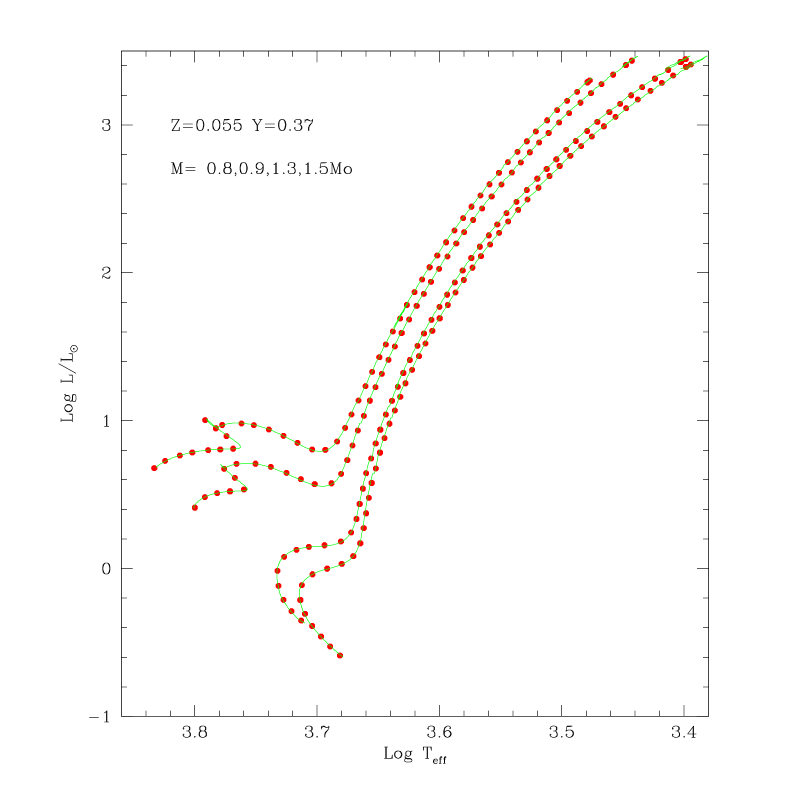
Figure 8: Comparison between computed evolutionary tracks (green line) for a chemical composition intermediate among those of the computed grids and the corresponding interpolated (red points) with the above described method for (Z=0.055,Y=0.37)

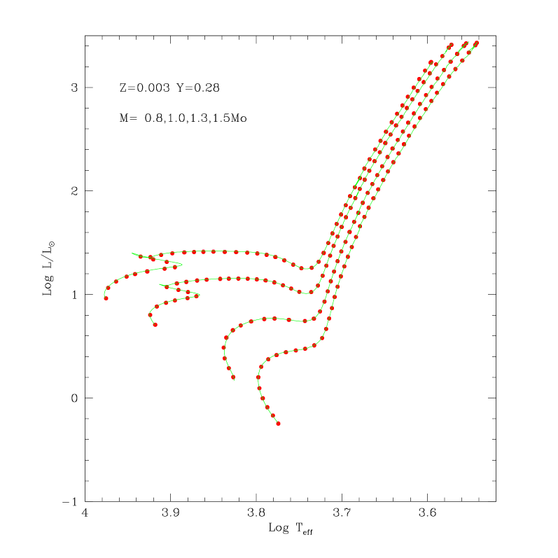
Figure 9: Comparison between computed evolutionary tracks (green line) for a chemical composition intermediate among those of the computed grids and the corresponding interpolated (red points) with the above described method for (Z=0.0003,Y=0.28)

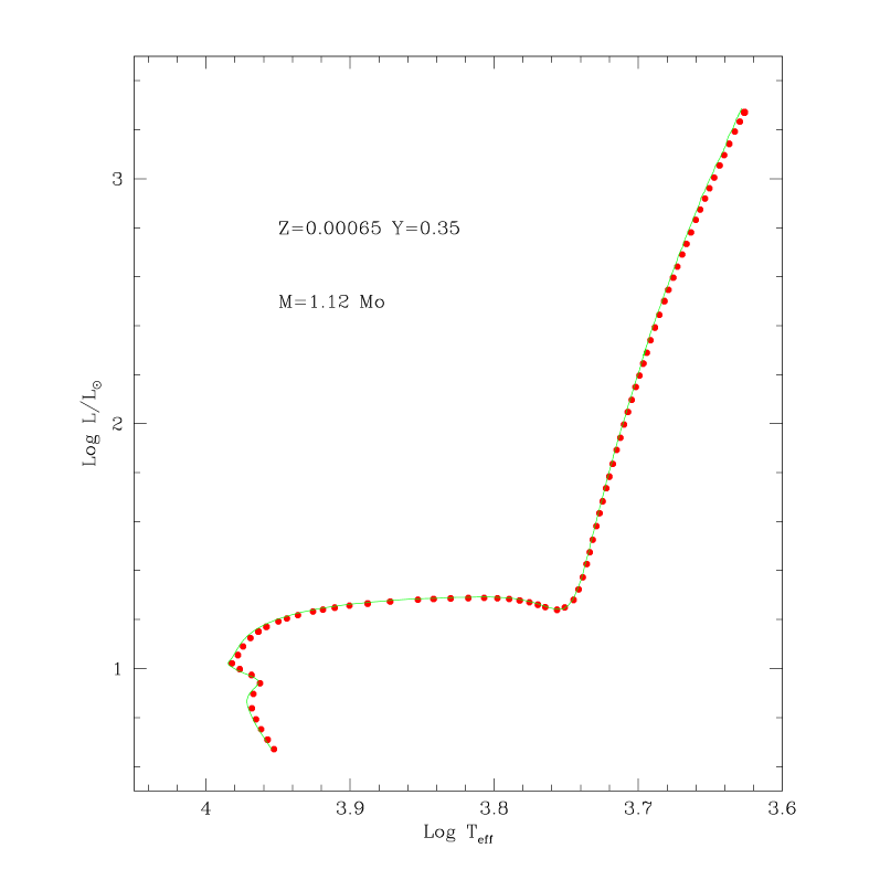
Figure 10: Comparison between a computed evolutionary track for $M=1.12M_{\odot}$ (green line) and the correspondent track obtained by interpolation from the grids (red points), with the chemical composition Z=0.00065 and Y=0.35, in the more complex case of close tracks with different morphology

We have done some tests in order to check the reliability of the method for the interpolation in the Z-Y plane. For a few combinations Z-Y we have calculated some tracks and then we have interpolated the same masses from the existing grids, using the new program YZVAR. The results of the comparison are shown in Figs.8, 9 and 10. In Fig. 8 for the chemical composition Z=0.055 and Y=0.37 (a point at the center of a mesh) we compare the computed evolutionary tracks of low mass stars of 0.8, 1.0, 1.3, 1.5 $M_{\odot}$ (green line) and those interpolated with YZVAR (red points). The result on the HR diagram is satisfactory and the ages differ by less than $1\%$. Fig. 9 presents the results as in Fig 8, but for the chemical composition Z=0.003 and Y=0.28. In Fig. 10 we display a critical case as the considered 1.12 $M_{\odot}$ is between two iso-phase intervals. In fact this mass is comprised between two masses with different morphology in the HR diagram. It is evident that the interpolation is able to reproduce the computed track very well.

5.3 Bolometric corrections

The present isochrones are provided in the Johnson-Cousins-Glass system as defined by Bessell (1990) and Bessell & Brett (1988). As soon as possible they will be available in the Vegamag systems of ACS and WFPC2 on board of HST (cf. Sirianni et al. 2005; Holtzman et al. 1995) and in the SDSS system. The formalism we follow to derive bolometric corrections in these systems is described in Girardi et al. (2002). The definition of zeropoints has been revised and is detailed in a forthcoming paper by Girardi et al. (in prep.; see also Marigo et al. 2007) and will not be repeated here.

Suffice it to recall that the bolometric correction tables stand on an updated and extended library of stellar spectral fluxes. The core of the library now consists of the “ODFNEW” ATLAS9 spectral fluxes from Castelli & Kurucz (2003), for $T_{\rm eff}$ between 3500 and 50000 K, $\log g$ between $-2$ and $5$, and scaled-solar metallicities [M/H] between -2.5 and +0.5. This library is extended at the intervals of high $T_{\rm eff}$ with pure blackbody spectra. For lower $T_{\rm eff}$, the library is completed with the spectral fluxes for M, L and T dwarfs from Allard et al. (2000), M giants from Fluks et al. (1994), and finally the C star spectra from Loidl et al. (2001). Details about the implementation of this library, and in particular about the C star spectra, are provided in Marigo et al. (2007) and Girardi et al. (in prep.).

It is also worth mentioning that in the isochrones we apply the bolometric corrections derived from this library without making any correction for the enhanced He content. As demonstrated in Girardi et al. (2007), for a given metal content, an enhancement of He as high as $\Delta Y=0.1$ produces changes in the bolometric corrections of just a few thousandths of magnitude. Just in some very particular situations, for instance at low $T_{\rm eff}$ and for blue pass-bands, can He-enhancement produce more sizeable effects on BCs; these situations however correspond to cases where the emitted stellar flux would anyway be very small, and therefore are of little interest in practice.

5.4 Description of isochrone tables

Complete tables with the isochrones can be obtained through the web site http://stev.oapd.inaf.it/YZVAR. In this data-base, isochrones are provided at $\Delta\log t=0.05$ intervals; this means that any two consecutive isochrones differ by only 12 percent in their ages.

For each isochrone table the corresponding data file presents 16 columns with the following information:

1. logAge: logarithm of the age in years;

2. log(L/Lo): logarithm of surface luminosity (in solar units);

3. logTef: logarithm of effective temperature (in K);

4. logG: logarithm of surface gravity (in cgs units);

5. Mi: initial mass in solar masses;

6. Mcur: actual stellar mass in solar masses;

7. FLUM: indefinite integral over the initial mass M of the Salpeter initial mass function by number;

8. - 15.: UBVRIJHK absolute magnitudes in the Johnson-Cousins-Glass system;

16. C.P.: index marking the presence of a characteristic point, when different from zero.

We recall that the initial mass is the useful quantity for population synthesis calculations, since together with the initial mass function it determines the relative number of stars in different sections of the isochrones. In column 7 the indefinite integral over the initial mass $M$ of the initial mass function (IMF) by number,

i.e.

$$\mbox{\sc flum}=\int\phi(M)\mbox{d}M$$ (1)

is presented, for the case of the Salpeter IMF, $\phi(M)=AM^{-\alpha}$, with $\alpha=2.35$. When we assume a normalization constant of $A=1$, flum is simply given by flum$=M^{1-\alpha}/(1-\alpha)$. This is a useful quantity since the difference between any two values of flum is proportional to the number of stars located in the corresponding mass interval. It is worth remarking that we present flum values for the complete mass interval down to 0.15 $M_{\odot}$, always assuming a Salpeter (1955) IMF, whereas we know that such an IMF cannot be extended to such low values of the mass. However, the reader can easily derive flum relations for alternative choices of the IMF, by using the values of the initial mass we present in Column 5 of the isochrone tables. In the last column when there appears the value 1, it marks the presence of a characteristic evolutionary point from the ZAMS to the beginning of the early AGB phase, while the value 2 is related to the characteristic points of the TP-AGB phase. If there is only one characteristic point (marked with 2) at the end of the isochrone, this means that the TP-AGB phase is very short. The beginning and the end of the TP-AGB phase are pointed out with index 2, as well as when C/O increases above unity (transition from M to carbon stars).

6 Comparison with other databases

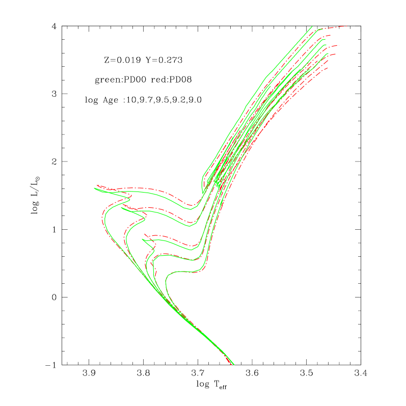
Figure 11: Comparison between the new Padova isochrones (PD08) and Girardi et al. (PD00) ones for Z=0.019 and Y=0.273 and log Age=10., 9.7, 9.5, 9.2, 9. years. Solid lines correspond to PD00, dash-dotted ones to PD08 isochrones.

a)

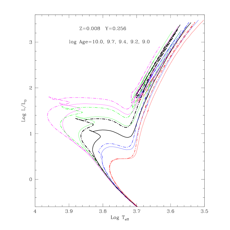
b)

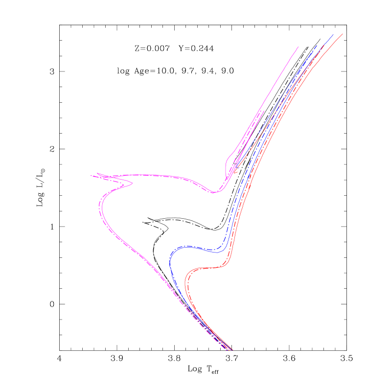
Figure 12: Comparison between Padova and Teramo isochrones with overshoot for the composition $[Z=0.008,Y=0.256]$ in panel a). Dot-dashed lines correspond to Teramo ones and solid lines to our new isochrones. The largest difference between the PD and Te isochrones is met at log Age=9.4. In panel b) the comparison is between Padova (solid line) and $YY$ isochrones (dot-dashed) with Z=0.007 and Y=0.244

a)

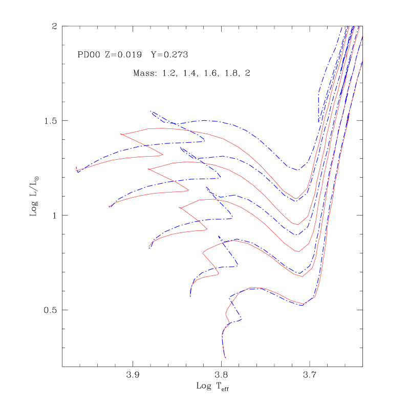
b)

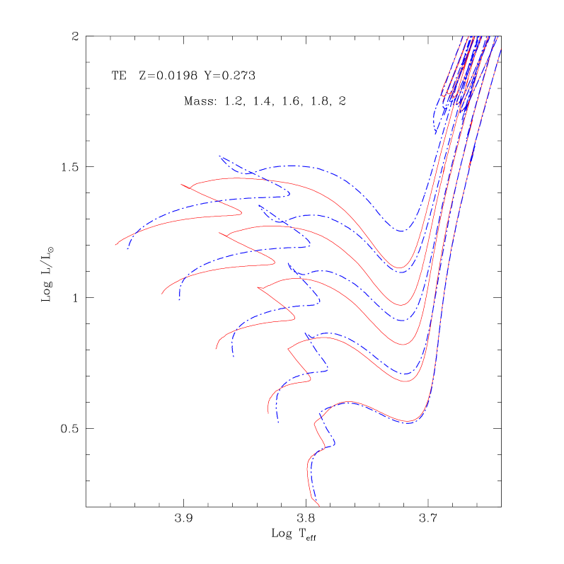
Figure 13: Evolutionary tracks from Girardi et al. (2000) for the composition $[Z=0.019,Y=0.273]$ with overshoot (dot-dashed line) and without (solid line) in panel a). In panel b) Teramo tracks are displayed for $[Z=0.0198,Y=0.273]$ with overshoot (dot-dashed line) and without (solid line). The ZAMS location for TE models with and without overshoot is not coincident.

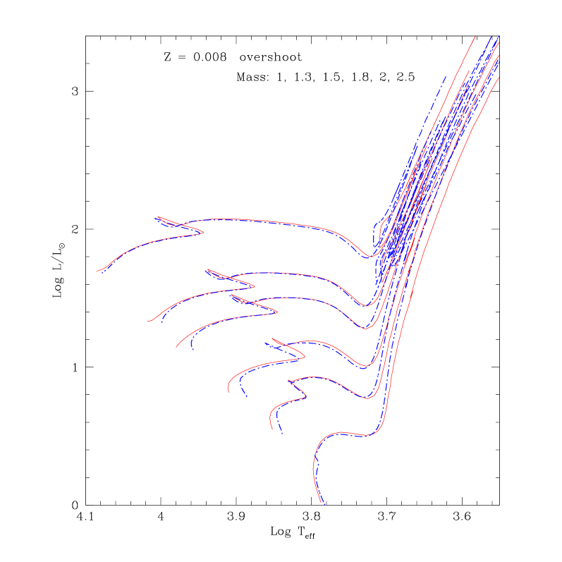
Figure 14: New Padova tracks and Teramo ones with overshoot from 1 to 2.5 $M_{\odot}$ for Z=0.008. Solid lines correspond to PD08 models, dash-dotted ones to Teramo tracks.

Table 4: Comparison of H-lifetimes for models with overshoot with nearly solar composition and for Z=0.008

$Z\sim Z_{\odot}$					$Z=0.008$
$M/\mbox{$M_{\odot}$}$	$t_{H}$ TE 1	$t_{H}$ PD08 2	$t_{H}$ $YY$ 3		$M/\mbox{$M_{\odot}$}$	$t_{H}$ TE 4	$t_{H}$ PD08 5	$t_{H}$ $YY$ 6
1.00	10.889	10.547	10.855		1.00	8.387	7.389	7.795
1.20	5.679	5.109	5.359		1.20	4.625	3.743	3.994
1.40	4.182	3.390	3.424		1.30	4.009	3.040	3.076
1.60	3.067	2.347	2.390		1.50	2.986	2.162	2.215
1.80	2.136	1.647	1.671		1.80	1.847	1.266	1.306
2.00	1.439	1.198	1.229		2.00	1.250	0.943	0.976
3.00	0.375	0.394	0.392		3.00	0.331	0.324	0.334
5.00	0.094	0.107	0.104		5.00	0.089	0.097	0.098

¹ Z=0.0198 Y=0.273; ² Z=0.017 Y=0.26; ³ Z=0.020 Y=0.27

⁴ Z=0.008 Y=0.256; ⁵ Z=0.008 Y=0.26; ⁶ Z=0.007 Y=0.244

Ages are in Gyr

Figure 11 shows the comparison between the isochrones by Girardi et al. (2000), hereafter PD00, with the new ones, hereafter PD08, in the age range between 1 and 14 Gyr, for the chemical composition $Z=0.017$ and $Y=0.273$. There are differences both in the MS phase and in the luminous part of the RGB and/or AGB phase. The main contribution to the differences in the MS phase is due to the interpolation technique for the opacity tables (see Section 2.2). The amount of the variation depends on mass and chemical composition. We have verified that low-mass stellar evolutionary tracks change very little with the method of opacity interpolation. For intermediate mass stars there is a lowering of the luminosity and a consequent increase of the lifetime of the new models. For values of log Age$\leq 9.5-9.7$ (it depends on the chemical composition) to obtain the same luminosity of PD00 for the MS termination point in the new isochrones (PD08) we must increase the logarithm of the age of about 0.05. The color of the turn-off of the new isochrones (younger than 9.5 Gyr) is bluer.

We point out that the luminous part of the RGB and/or AGB phases in the new isochrones is redder than in PD00 ones and the separation increases for increasing luminosity. This effect is due to the treatment of the density inversion in the red giant envelope. In the outermost layers of stars with $T_{eff}\leq 10^{4}K$ a convective zone develops caused by the incomplete ionization of hydrogen. If convection is treated according to the mixing-length theory (MLT) with the mixing-length proportional to the pressure scale height ($H_{p}$), when $T_{eff}\leq 10^{4}K$ a density inversion occurs. This situation might be unphysical and it has been the subject of many speculations. This difficulty can be avoided by adopting the density scale height $H_{\rho}$ instead of $H_{p}$ in the MLT. Really in Girardi et al. tracks we avoided the inversion density imposing that the temperature gradient $\Delta T$ is such that the density gradient obeys the condition $\Delta_{\rho}\geq 0$. However the comparison of the PD00 isochrones with the observations seems to require redder RGB and/or AGB branches. For this reason in the present computations we have used the MLT proportional to the pressure scale height, allowing the inversion density in the red convective envelope, as already adopted in Bertelli et al. (1994) isochrones. The presence of the inversion density determines RGB and/or AGB phases redder than in previous isochrones (PD00).

Neutrino cooling is also more efficient during the RGB phase in the new tracks, as described in Section 2.4 and it contributes to make the tip of the RGB more luminous than in PD00. We have verified that for Z in the range 0.0001 - 0.001 (low values of Y) and for the solar case the overluminosity is of the order 0.12 - 0.15 in units of $logL/L_{\odot}$ (the considered ages are around log Age=10.0). The effect on the I magnitude consists in an overluminosity of the order of between -0.20 and -0.35 for Z in the range 0.0001 - 0.001. On the other hand in the solar case the interplay between lowering effective temperature and increasing bolometric corrections is such that the tip of the PD00 case appears to be approximately one magnitude more luminous than the new one, inverting what happens to the I magnitude for low values of Z.

The comparison of some selected tracks and isochrones of the new grids of the Padova database(PD08) with the analogous counterparts of the publicly available Teramo database (TE) by Pietrinferni et al. (2004) and the $YY$ database by Yi et al. (2001) and Demarque et al. (2004) pointed out some differences.

As already evident in the comparison of isochrones by different groups, shown in Pietrinferni et al. (2004), there is a systematic difference from their 1.8 Gyr isochrone and the one by Girardi et al. (2000) and by Yi et al. (2001), as for the 2.0 Gyr one by VandenBerg (see figures 8, 11 and 12 in Pietrinferni et al. 2004). In fact the turn-off luminosity of their 1.8 Gyr isochrone (or 2.0 in the comparison with VandenBerg) is higher, whereas the 10 Gyr and the 0.5 Gyr ones are practically the same as by the other groups. They ascribed the differences to differences in input physics and in the overshooting treatment relatively to the comparison with Girardi et al. (2000).

In Table 4 we compare the H-lifetimes for models with overshoot in the mass range between 1 and 5 $M_{\odot}$ and with a chemical composition approximately solar We point out that the largest differences can be found in the range between 1 and 2 solar masses, in the sense that while PD08 and $YY$ tracks have similar H-lifetimes, TE models are systematically longer up to 0.8 Gyr. This difference cannot be ascribed to the treatment of overshoot, in fact both groups (PD and TE) assume a similar prescription in the range between 1 and 2 $M_{\odot}$ (the core overshoot efficiency decreases linearly from about $1.7-1.5M_{\odot}$ down to $1M_{\odot}$, where the efficiency is zero for stars with a radiative core).

The recent determination of the age of the LMC globular cluster NGC 1978, studied by Mucciarelli et al. (2007) shows the same anomaly, in this case for the chemical composition typical of the LMC. The authors find that the age obtained with Teramo isochrones results significantly older than that obtained with Pisa and Padova isochrones, even if the same amount of overshoot is assumed in the considered models. Comparing the H-lifetimes for $Z=0.008$ we notice that there is a very satisfactory agreement between the H lifetimes of $YY$ and PD08, whereas TE ages are older up to about 1 Gyr at about $1.3M_{\odot}$. The largest differences are present in the range between 1 and 2 $M_{\odot}$, as shown in Table 4.

Figure 12 panel a) shows isochrones (at log Age = 10.0, 9.7, 9.4, 9.2, 9.0 years) from Teramo database with Z=0.008 and Y=0.256, and (interpolated at the same metal and helium content) from our new isochrones. This figure remarks the difference in luminosity of the isochrones for the same age from the two databases, more evident for log Age=9.4 (black solid line for PD08 and black dash-dotted for Teramo) in the color version of the electronic paper. In panel b) we compare Padova new isochrones for Z=0.007 and Y=0.244 with $YY$ and we find out that the agreement is very good, considering that their models take into account convective core overshoot (0.2) and helium diffusion (PD08 and $YY$ isochrones are shown for log Age = 10.0, 9.7, 9.4 and 9.0 years).

The reasons of the above mentioned disagreement cannot be easily disentangled, but we notice that the ZAMS models for PD00 tracks (Girardi et al. 2000 for solar chemical composition) with and without overshoot are coincident (as the ZAMS is the location of chemically homogeneous models for the various considered masses), while they are different in luminosity and temperature for Teramo ones between 1 and 2 $M_{\odot}$. The difference in the location of ZAMS models can be seen also in Figure 14 where we plot our new models and Teramo ones with overshoot for Z=0.008.

In Figure 13 the PD00 and TE tracks are plotted in the range of mass between 1.2 and 2 $M_{\odot}$. As we did not compute new tracks without overshoot, we plotted PD00 and TE models with and without overshoot to make a comparison. The anomalously longer H-burning lifetimes of TE models with respect to other authors is probably, at least partly, related to the lower luminosiy of the beginning of the central H-burning for their models with overshoot. We point out that Teramo models with overshoot were computed starting from the pre-MS phase for masses lower than $3M_{\odot}$. Anyway also $YY$ models were evolved from the pre-MS stellar birthline to the onset of helium burning (Yi et al. 2001), but there are not significant differences (comparing PD08 to YY results) in the H-lifetimes and for the isochrones in the age range between 1 and 10 Gyr, as shown in Table 4 and Figure 12 b).

7 Concluding remarks

Large grids of homogeneous stellar evolution models and isochrones are a necessary ingredient for the interpretation of photometric and spectroscopic observations of resolved and unresolved stellar populations. Appropriate tools to compute synthetic color-magnitude diagrams for the analysis of stellar populations require also the selection of the chemical composition to be used in the simulation. Evolutionary stellar models are usually computed taking into account a fixed law of helium to metal enrichment. Determinations of the helium enrichment $\Delta Y/\Delta Z$ from nearby stars and K dwarfs, or from Hyades binary systems show a large range of values for this ratio. Recent results suggest that the naive assumption that the helium enrichment law is universal, might not be correct. In fact there has been recently evidence of significant variations in the helium content (and perhaps of the age) in some globular clusters, like $\omega$ Cen, NGC 2808 and NGC 6441, while globular clusters were traditionally considered as formed of a simple stellar population of uniform age and chemical composition.

These results prompted us to compute new stellar evolutionary tracks covering an extended region of the plane Z-Y, in order to enable users to analyse stellar populations with different helium enrichment laws.

In this paper we present 39 grids of stellar evolutionary tracks up to $2.5M_{\odot}$. Next paper will present tracks and isochrones from $2.5$ up to $20M_{\odot}$ for the same grid of chemical compositions. The typical mass resolution for low mass stars is of 0.1 $M_{\odot}$, reduced to $0.05$ in the interval of very low masses ($M<0.6M_{\odot}$), and occasionally in the vicinity of the separation mass $M_{Hef}$ between low and intermediate mass stars. In this way we provide enough tracks to allow a very detailed mapping of the HR diagram and the relative theoretical isochrones are also very detailed. An important update of this database is the extension of stellar models and isochrones until the end of the TP-AGB by means of new synthetic models (cf. Marigo & Girardi 2007). The results of these new grids allow the estimate of several astrophysical quantities as the RGB transition mass, the He core mass at He ignition, the amount of changes of chemical elements due to the first dredge-up, and the properties of the models at the beginning of the thermal pulse phase on the AGB.

The web site (http://stev.oapd.inaf.it/YZVAR), dedicated to make available the whole theoretical framework to the scientific community, includes:

• Data files with the information relative to each evolutionary track

• Isochrone files with the chemical composition of the computed grids in the Z-Y plane

Every file contains isochrones with $\sim 10.15\leq$ Log Age $\leq\sim 9.0$ years with time step equal to 0.05. The initial and the final value can be a little more or a little less, dependent on the chemical composition. To compute the isochrones we adopted the interpolation scheme described in Section 5.1. A web interactive interface will be tuned up as soon as possible to allow users to obtain isochrones of whatever chemical composition inside the original grid.

A modified version of the program which computes the isochrones is suited to the purposes of evolutionary population synthesis, either of simple (star clusters) or complex stellar populations (galaxies). In the latter case it is possible to select the kind of star formation history, the chemical enrichment law in the plane Z-Y, the initial mass function and the mass loss rate during the RGB phase. The previous program ZVAR, in which the helium enrichment law was implicit in the chemical composition of the various evolutionary sets, is now updated for being used in the extended region of the Z-Y plane and is named YZVAR. A web interactive interface will provide stellar populations for selected input data for the SFR, IMF, chemical composition and mass loss during the RGB phase.

- (1) Alexander, D.R. & Ferguson, J.W. 1994, ApJ, 437, 879
- (2) Allard, F. et al. 2000, in From giant planets to cool stars, ASP Conf. Ser. 212, eds. C.A. Griffith & M.S. Marley, p. 127
- (3) Alongi, M., Bertelli, G., Bressan, A., Chiosi, C., 1991, A&A, 244, 95
- (4) Anders, E. & Grevesse, N. 1989, Geochim. Cosmochim. Acta, 53, 197
- (5) Antia, H.M. & Basu, S. 2006, ApJ, 644,1292
- (6) Aparicio, A., Gallart, C., Chiosi, C., Bertelli, G. 1996, ApJ, 469, L97
- (7) Asplund, M. et al. 2005, A&A, 431.693
- (8) Asplund, M., Grevesse, N., Sauval, A.J. 2006, Comm. in Asteroseismology, Vol. 147, p.76
- (9) Bahcall, J.N., Serenelli, A.M., Basu, S. 2006, ApJS, 165, 400
- (10) Bertelli, G. et al. 1990, A&AS, 85, 845
- (11) Bertelli, G., Bressan, A., Chiosi, C., Fagotto, F., Nasi, E. 1994, A&AS, 106, 275
- (12) Bertelli, G. & Nasi, E. 2001, AJ, 121, 1013
- (13) Bertelli, G., Nasi, E., Girardi, L. et al. 2003, AJ, 125, 770
- (14) Bessell, M.S. 1990, PASP, 102, 1181
- (15) Bessell, M.S. & Brett, J.M. 1988, PASP, 100, 1134
- (16) Böhm-Vitense, E. 1958, Z. Astroph., 46, 108
- (17) Bowen, G.H. & Willson, L.A. 1991, ApJ, 375, L53
- (18) Bressan, A., Bertelli, G., Chiosi, C. 1981, A&A, 102, 25
- (19) Bressan, A., Fagotto, F., Bertelli, G., Chiosi, C. 1993, A&AS, 100, 647
- (20) Caloi, V. & D’Antona, F. 2007, A&A, 463, 949
- (21) Casagrande, L. et al. 2007, astro-ph/0703766
- (22) Castellani, V. et al., 1985, ApJ, 296, 204
- (23) Castelli, F. & Kurucz, R.L. 2003, in Modelling of Stellar Atmospheres, IAU Symp. 210,eds. N.E. Piskunov et al., p. 20 (San Francisco: ASP)
- (24) Caughlan, G.R. & Fowler, W.A. 1988, Atomic Data Nucl. Data Tables, 40, 283
- (25) Chiosi, C., Bertelli, G., Bressan, A. 1992, ARA&A, 30, 305
- (26) Claret, A. 2007, A&A, 475, 1019
- (27) D’Antona, F. et al. 2005, ApJ, 631, 868
- (28) D’Antona, F. & Ventura, P. 2007, MNRAS, 379, 1431
- (29) Däppen, W., Mihalas, D., Hummer, D.G., Mihalas, B.W. 1988, ApJ, 332, 261
- (30) Deng, L. & Xiong D. R. 2007, astro-ph/0707.0924
- (31) Demarque, P., Woo, J.-H., Kim, Y.-C., Yi, S. K. 2004, ApJS, 155, 667
- (32) Dotter, A., Chaboyer, B., Jevremovic, D. et al. 2007, AJ, 134, 376
- (33) Fagotto, F., Bressan, A., Bertelli, G., Chiosi, C. 1994a, A&AS, 104, 365
- (34) Fagotto, F., Bressan, A., Bertelli, G., Chiosi, C. 1994b, A&AS, 105, 29
- (35) Fluks, M.A. et al. 1994, A&AS, 105, 311
- (36) Fox, M.W. & Wood, P.R. 1982, ApJ, 259, 198
- (37) Girardi, L., Bressan, A., Chiosi, C., Bertelli, G., Nasi, E. 1996, A&AS, 117, 113
- (38) Girardi, L., Bressan, A., Bertelli, G., Chiosi, C. 2000, A&AS, 141, 371
- (39) Girardi, L. et al. 2002, A&A, 391, 195
- (40) Girardi, L., Castelli, F., Bertelli, G., Nasi, E. 2007, A&A, 468, 657
- (41) Girardi, L. & Marigo, P. 2007, astro-ph 0701533
- (42) Graboske, H.C., de Witt, H.E., Grossman, A.S., Cooper, M.S. 1973, ApJ, 181, 457
- (43) Grevesse, N. & Noels, A. 1993, Phys. Scr. T, 47, 133
- (44) Grevesse, N. & Sauval, A.J. 1998, Space Sci. Rev., 85, 161
- (45) Haft, M., Raffelt, G. & Weiss, A. 1994, ApJ, 425, 222
- (46) Holtzman, J.A. et al. 1995, PASP, 107, 1065
- (47) Hubbard, W.B. & Lampe M. 1969, ApJS, 18, 297
- (48) Hummer, D.G. & Mihalas D. 1988, ApJ, 331, 794
- (49) Iglesias, C.A. & Rogers, F.J. 1996, ApJ, 464, 943
- (50) Itoh, N. & Kohyama, Y. 1983, ApJ, 275, 858
- (51) Itoh, N., Mitake, S., Iyetomi, H., Ichimaru, S. 1983, ApJ, 273, 774
- (52) Izzard, R.G. et al. 2004, MNRAS, 350, 407
- (53) Jimenez, R. et al. 2003, Science, 299, 1552
- (54) Karakas, A.I., Lattanzio, J.C., Pols, O.R. 2002, PASA, 19, 515
- (55) Karakas, A.I., Fenner, Y., Sills, A. et al. 2006, ApJ, 652, 1240
- (56) Kunz, R., Fey, M., Jaeger, M. et al. 2002, ApJ, 567, 643
- (57) Landré, V., Prantzos, N., Aguer, P., Bogaert, G., Lefebvre, A., Thibaud, J.P. 1990, A&A, 240, 85
- (58) Lebreton, Y. et al. 2001, A&A, 374, 540
- (59) Lee, Y.-W. et al. 2005, ApJ, 621, L57
- (60) Loidl, R., Lancon, A., Jorgensen, U.G. 2001, A&A, 371, 1065
- (61) Maeder, A.& Meynet, G. 2006, A&A, 448, L37
- (62) Marigo, P. 2002, A&A, 387, 507
- (63) Marigo, P. et al. 2001, A&A, 371, 152
- (64) Marigo, P., Girardi, L., Chiosi, C. 2003, A&A, 403, 225
- (65) Marigo, P.& Girardi, L. 2007, A&A, 469, 239
- (66) Marigo, P. et al. 2007, A&A submitted
- (67) Meynet, G., Maeder, A., Schaller, G., Schaerer, D., Charbonnel, C. 1994, A&AS, 103, 97
- (68) Mihalas, D., Däppen, W., Hummer, D.G. 1988, ApJ, 331, 815
- (69) Mihalas, D., Hummer, D.G., Mihalas, B.W., Däppen, W. 1990, ApJ, 350, 300
- (70) Montalban, J. et al. 2006, Comm. in Asteroseismology, Vol. 147, p. 80
- (71) Mucciarelli, A., Ferraro, F., Origlia, L. et al. 2007, AJ, 133, 2053
- (72) Munakata, H., Kohyama, Y., Itoh, N. 1985, ApJ, 296, 197
- (73) Ng, Y. K., Bertelli, G., Bressan, A. et al. 1995, A&A, 295, 655
- (74) Ostlie, D.A. & Cox, A.N. 1986, ApJ, 311, 864
- (75) Pagel, B.E.J. & Portinari, L. 1998, MNRAS, 298, 747
- (76) Pietrinferni, A., Cassisi, S., Salaris, M., Castelli, F. 2004, ApJ, 612, 168
- (77) Pietrinferni, A., Cassisi, S., Salaris, M., Castelli, F. 2006, ApJ, 642, 797
- (78) Piotto, G. et al. 2005, ApJ, 621, 777
- (79) Piotto, G., Bedin, L. R., Anderson, J., et al. 2007, ApJ, 661, L53
- (80) Prantzos, N. & Charbonnel, C. 2006, A&A, 458, 135
- (81) Reimers, D. 1975, Mem. Soc. R. Sci. Liege, ser. 6, vol. 8, p. 369
- (82) Renzini, A. & Fusi-Pecci, F. 1988, ARA&A, 26, 199
- (83) Rogers, F.J., Swenson, F.J., Iglesias, C.A. 1996, ApJ, 456, 902
- (84) Salasnich, B., Girardi, L., Weiss, A., Chiosi, C., 2000, A&A, 361, 1023
- (85) Salpeter, E.E. 1955, ApJ, 121,161
- (86) Schlattl, H. & Weiss, A. 1998, in Proc. Neutrino Astrophysics, Ringberg Castle, Germany, Oct 1997, eds. M. Altmann, W. Hillebrandt et al.
- (87) Sirianni, M. et al. 2005, PASP, 117, 1049
- (88) Spergel, D.N. et al. 2003, ApJS, 148, 175
- (89) Spergel, D.N. et al. 2007, ApJS, 170, 377
- (90) VandenBerg, D.A., Bergbusch, P.A., Dowler, P.D. 2006, ApJS, 162, 375
- (91) VandenBerg, D.A. et al. 2007, ApJ, 666, L105
- (92) Vemury, S.K., Stothers, R. 1978, ApJ, 225, 939
- (93) Villanova, S., Piotto, G., King, I.R. et al. 2007, ApJ, 663, 296
- (94) Wachter, A. et al. 2002, A&A, 384, 452
- (95) Wagenhuber, J. & Groenewegen, M.A.T. 1998, A&A,340, 183
- (96) Weaver T.A. & Woosley S.E. 1993, Phys. Rep., 227, 65
- (97) Weiss, A. & Schlattl, H. 2000 A&AS, 144, 487
- (98) Weiss, A., Keady, J.J., Magee, N.H. Jr. 1990, Atomic Data and Nuclear Data Tables, 45, 209
- (99) Yi, S., Demarque, P., Kim, Y.-C. et al. 2001, ApJS, 136, 417